Experimental and Numerical Investigations of the Sediment Abrasion Mechanism at the Leading Edge of an Airfoil

Abstract

Multiple engineering projects have confirmed that hydraulic machinery operating in sediment-laden rivers undergoes sediment abrasion. Guide vanes are among the most severely worn flow-passing components and have long been a key research focus in hydraulic machinery. In this research, a wear test of the NACA0012 cascade under a 10° incoming flow angle was carried out in the Venturi test system, and the evolution process of the wear was analyzed. The three-dimensional flow channel of the cascade was constructed, and the Finnie wear model was adopted for computational fluid dynamics (CFD) simulations to analyze the wear mechanism at the initial stage. The results indicate that abrasion primarily occurs at the airfoil’s leading edge and progresses through three stages: initiation, development, and stabilization. The calculated results closely matched the latest wear outcomes: In the initial stage, the wear rate density was influenced by the particle impact velocity, angle, volume fraction, and y-direction shear stress. A low-velocity zone near the impact point, combined with rebounding particles causing secondary impacts, increases the particle volume fraction and wear rate density. These secondary impacts are the primary causes of erosion on both the upstream and downstream surfaces. Furthermore, flow separation downstream from the leading edge makes this region highly susceptible to wear. This study provides valuable insights for addressing wear in hydraulic machinery for practical engineering applications.

1. Introduction

Sediment abrasion has long been a significant concern in hydraulic machinery because it causes wear and deformation of the flow-passing components and leads to performance degradation, which affects the stability and safe operation of the units. In recent years, high-head and large-capacity hydraulic turbines have been successfully implemented in the mountainous regions of Southwest China. Wear failures of these units have resulted in significant economic losses and safety risks. Therefore, it is crucial to address and prevent wear in hydraulic machinery [1].

Hydraulic machinery operating in sediment-laden rivers undergoes severe wear, particularly in turbine guide vanes (TGVs). In recent years, many scholars have extensively investigated the factors influencing the wear of the flow passage components of hydraulic machinery through methods such as tests and computational fluid dynamics (CFD) simulations. The research indicates that the wear is mainly affected by the property parameters of sediment particles (hardness, size, concentration, and density), the velocity of the sediment-laden water flow, and the material’s characteristics [2,3,4].

Zhang Guang [5] applied the multiphase flow model of solid–liquid two-phase fluids to numerically calculate the flow in the guide vane region under various sediment medium conditions and analyzed the effects of sediment properties on the pressure distribution and sediment concentration regularities in the guide vane. Chen [6], aiming at the large eccentric shaft of the guide vane, carried out numerical computations by adopting a large eddy simulation and a discrete phase model and investigated the erosion characteristics and mechanisms of the end-surface of the guide vane and head cover, as well as the flow mechanism behind the guide vane. It was found that von Kármán vortex streets are the primary cause of unfavorable erosion behind the shaft and that the low-frequency energy of the turbulence plays a leading role in the erosion process. Han [7], Rakibuzzaman [8], and Lu [9] employed the k-ε turbulence model and DPM to investigate the sand particle erosion characteristics of the guide vane, identified the main erosion zone of the guide vane, and found that it was in accordance with the experimental erosion results. Chen [10] and Shrestha [11] carried out a comprehensive study of the influences of particulate property parameters on the wear rates of flow passage components. Characteristics such as the density, shape, size, and concentration of particles have direct impacts on the wear. Under the condition that the concentration and particle size of the particles are the same, the increase in the particle density leads to reductions in the sediment content, erosion rate, and erosion area. In addition, the shape and concentration of the particles have the most significant influences on the wear. Zhang Lei [12] used the two-phase flow model to investigate the effects of operating conditions on the wear in the guide vane region and analyzed the pressure, flow velocity, and sediment content in the guide vane region under different operating conditions. The results indicate that the operating conditions have significant impacts on the two-phase flow in the guide vane. With the decrease in the output of the hydraulics, the maximum flow velocity in the guide vane actually increases, and the speed difference between the leading and trailing surfaces of the movable guide vane also gradually increases.

The above-mentioned research mainly adopts numerical simulations to consider the sediment wear issue of guide vanes in various aspects. For instance, sediment abrasion is investigated in terms of the size of particles and the flow around guide vanes, and the influences of different working conditions on the solid–liquid two-phase flow pattern around the movable guide vanes are also examined. Because of the synergistic effects of sediment parameters (such as morphology, particle size, concentration, hardness, and flow velocity), precisely predicting the sediment abrasion of guide vanes is challenging.

Because of the limitations of numerical simulation models, there is a certain deviation between the calculated results and actual erosion. In order to reveal the mechanism of the particle erosion, it is necessary to conduct sediment erosion tests for verification. In terms of model experiments, Thapa [13] and Koirala [14] designed a three-guide-vane test rig using PIV to measure the velocity and pressure within guide vane gaps. Their tests visualized the flow behavior in the gaps and demonstrated that the pressures on both sides of the blade and at the exit were positively correlated with the wear levels. Brekke [15] categorized guide vane wear into four types based on guide vane flow characteristics: turbulent, secondary flow, leakage, and accelerated scours. Song [16] investigated the influences of a guide vane opening on particle motion and sediment erosion in a runner chamber and concluded that guide vane openings increase the flow rates in gapless channels. Lu [9], Yao [17], and Zhao [18] used CFD simulations of two-phase flow fields to extract wall profiles and designed a novel test rig to examine the wear zones on fixed guide vanes under rated conditions. They conducted sediment wear tests on the turbine guide vanes and developed a predictive model for sediment wear. Thapa [19] designed a single guide vane passage with a fluid field distribution similar to that of the prototype turbine. The fluid conditions at the guide vane’s inlet were measured when the gap between the guide vane and the panel was 2 mm. The results indicated that the relative velocity near the shroud at the inlet of the guide vane would increase to three times its nominal value and form a vortex filament at the guide vane’s inlet, which entered the runner along with the main stream. Turbine guide vanes (TGVs) region belongs to the annular cascade, the passage of water and sediment through the cascade generates an uneven flow field, resulting in variations in the distribution of solid particles and, thus, different erosion patterns at different positions of the guide vane.

According to the above research, scholars have carried out numerous studies on the prediction of erosion and discovered that the movement characteristics of particles in the near-wall region are highly correlated with the occurrence of wear [20]. However, the generation of sediment erosion is cumulative, and, thus, research on the process of wear development is lacking. In this paper, a cascade similar to the guide vanes of a turbine was designed for the experimental study of the erosion mechanism. The cascade was composed of five NACA0012 airfoils made of an aluminum alloy. The erosion evolution process of the cascade under the condition of a Reynolds number of 8.0 × 10⁵ is explored. Combined with numerical simulations, the results were cross-validated using the Finnie model to address the challenge of capturing near-wall flow fields during tests. This study examined the effects of solid-phase impact and near-wall flow field characteristics on wear generation, providing practical insights for addressing wear issues in engineering applications.

2. Materials and Methods

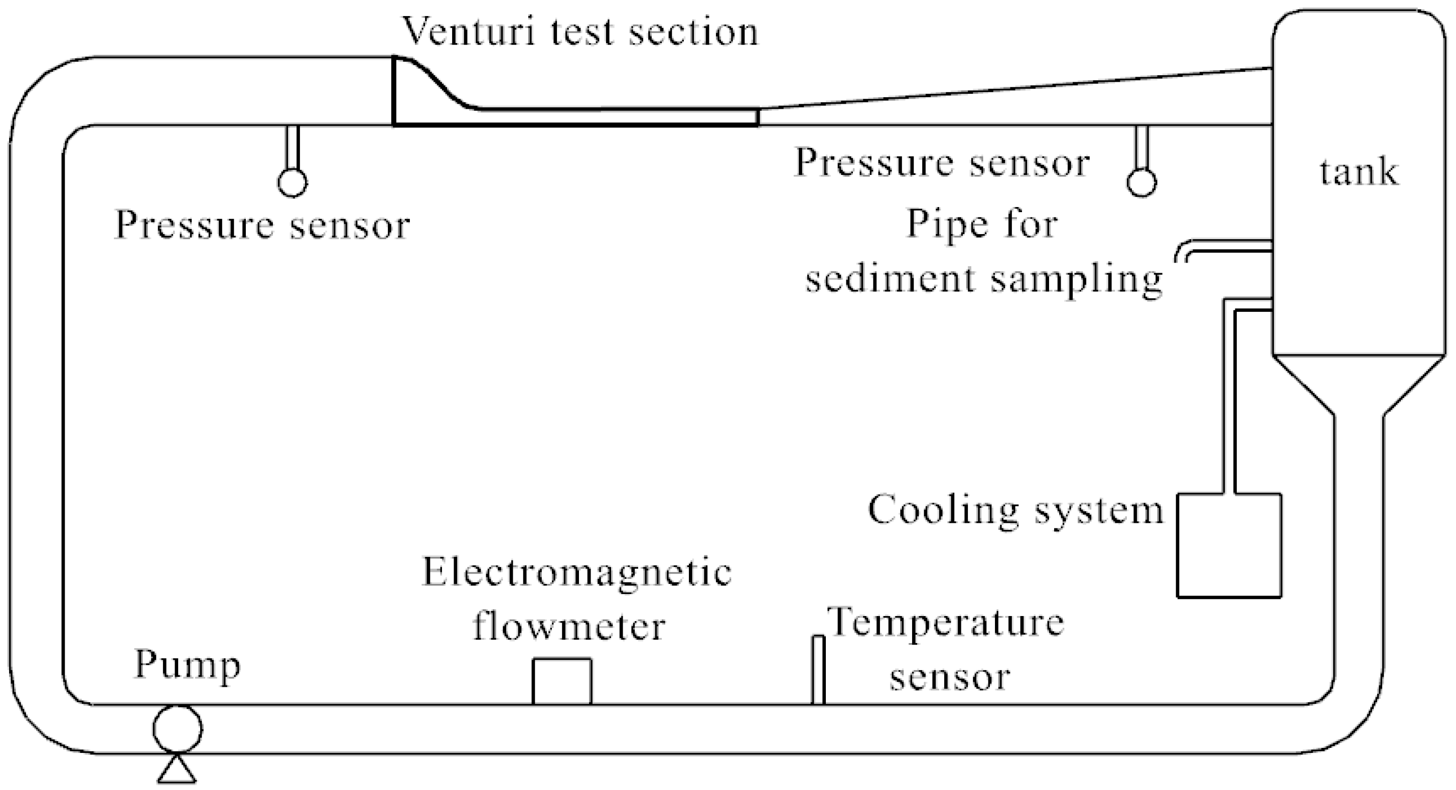
2.1. Introduction to the Tests

The tests were conducted using a Venturi abrasion test system primarily designed for sediment abrasion testing. An aluminum alloy airfoil was selected to examine the evolution of the wear damage on the vane cascade under an incoming flow with a 10° impact angle. The layout of the Venturi wear test cycle system for a vane cascade is shown in Figure 1. The Venturi abrasion test setup is shown in Figure 2. The actual image of the experimental section part with a proper scale bar is depicted in Figure 3.

2.1.1. Test Conditions

To replicate the actual flow conditions of the guide vanes and ensure a smooth, fully developed turbulence upstream from the airfoil, a long test section design was used. The distances between the test section’s inlet and outlet and the center of rotation of the intermediate airfoil (25 mm from the leading edge) were L1 = 575 mm and L2 = 700 mm, respectively. In addition, to accurately simulate the periodic boundary conditions of the guide vane, numerical simulations of the flow characteristics of the vane cascade in a clean water field were conducted under the same test conditions. Smooth streamlines near the airfoil’s wall were extracted and used as profiles for the inner walls of the test flow channel to reduce the effect of the flow channel’s walls on the flow characteristics of the vane cascade. Five NACA0012 airfoils, each with a chord length (c) of 100 mm, were fixed at equal intervals, with a blade spacing (d) of 40 mm in the test section’s flow channel, as shown in Figure 4. The mechanical properties and chemical composition of the test specimen material are listed in

Table 1. Mechanical properties of the specimen material.

Material	Hardness	Tensile Strength, σb (MPa)	Conditional Yield Strength, σ0.2 (MPa)	Elongation, δ5 (%)
Aluminum alloy	90–95 HBW	180	110	14

and

Table 2. The chemical composition of the test specimen material (aluminum alloy).

Element	Cu	Mn	Mg	Zn	Cr	Ti	Si	Fe	Al
Mass fraction	0.15–0.4	0.15	0.8–1.2	0.25	0.04–0.35	0.15	0.4–0.8	0.7	Remainder

. The incoming flow angle (α) was 10°, and the incoming flow velocity was 8 m/s, corresponding to a Reynolds number of 8.0 × 10⁵. The mass concentration (C_m) of the sediment in the test water was approximately 6.0 kg/m³, with a volume fraction (C_V) of approximately 0.28%, as detailed in

Table 3. Test conditions.

Re	Impact Angle, α	Sediment Mass Concentration, Cm (kg/m3)	Sediment Volume Fraction, CV (%)	Average Sediment Concentration (kg/m3)	Median Particle Size (μm)
8.0 × 105	10°	6.0	0.28	5.61	65.9

.

2.1.2. Test Methods

Wear tests were conducted under non-cavitation conditions. Before each test, approximately 8.0 kg of sediment was added to each test group, calculated based on the water volume of the system. During the test, two samples of sediment-laden water were collected, and the actual sediment content was determined by averaging these samples. The average sediment concentration is approximately 5.61 kg/m³.

To minimize errors owing to sediment wear and the system’s temperature rise, each test cycle lasted for 6 h. At the end of each cycle, the test system was stopped, the water and sediment were drained, and fresh water and sediment were added for the next cycle. Four tests were conducted in each group to observe the evolution of the sediment wear, totaling a net wear time of 24 h. After each group, the airfoil was removed, and its surface profile was measured using a surface profiler with an accuracy of 0.1 μm. The weight loss of the airfoil was also measured using an analytical balance, with an accuracy of 0.1 mg, to assess changes in both the surface profile and mass. The first set of tests lasted for 12 h to determine the initial wear position, followed by five additional cycles for 24 h each, resulting in a total test duration of 132 h.

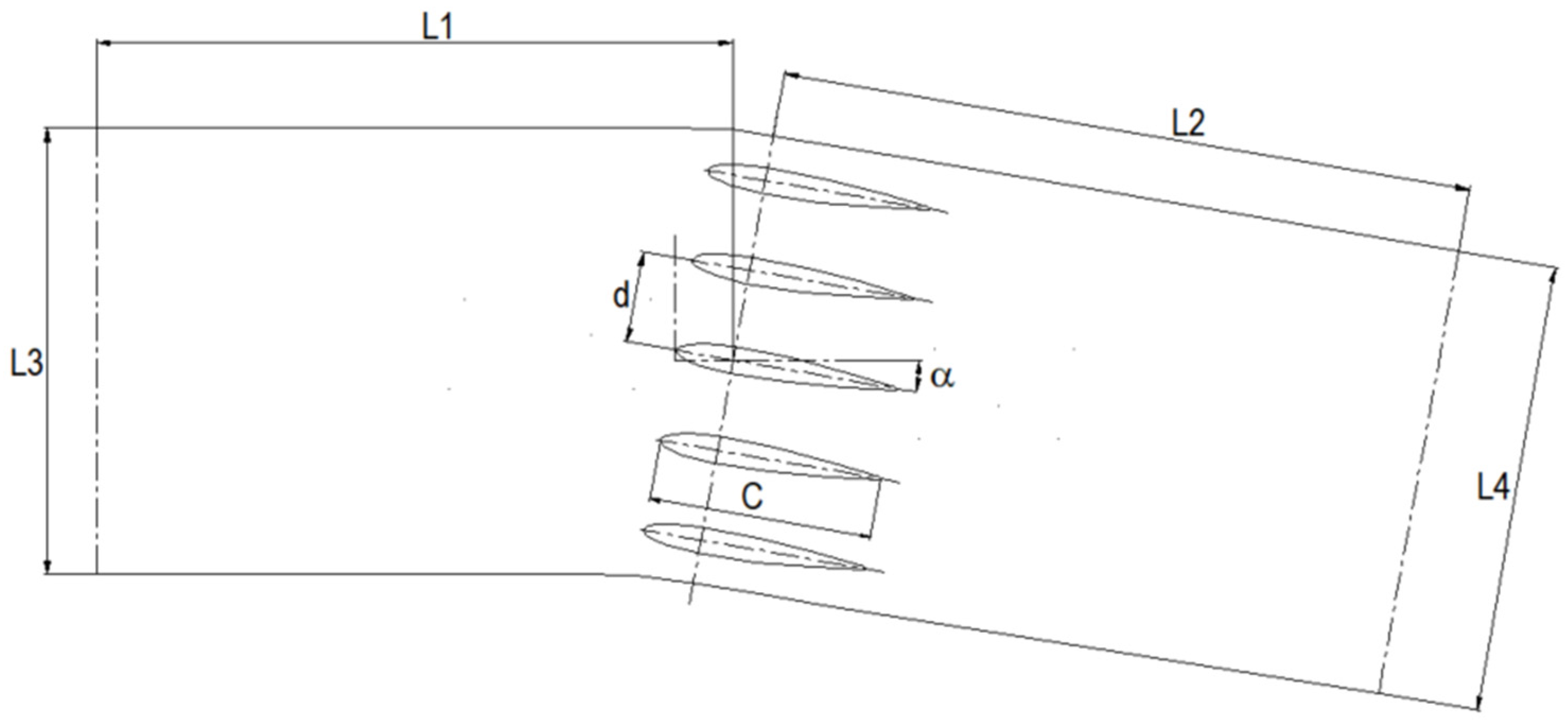
2.1.3. Measurement of the Airfoil’s Outer Profile

The surface profiler uses white-light confocal technology to measure distances. The model of the surface profiler is ST400Z, which is manufactured by NANOVEA. Following the scanning measurement protocol, a linear scanning method was employed in the x-direction. After each line scan, the stage was moved in the y-direction using a predetermined step size to scan the next line. The scanning step sizes in the x-direction and y-direction achieved an accuracy of 0.1 μm, as shown in Figure 5. The z-axis measurement range was set at 10 mm. To address the profiler’s depth measurement limitations, particularly the high-curvature surface profile of the airfoil’s leading edge, which exceeded the instrument’s measurement range, a motorized rotary table was installed on the stage to provide an additional rotational degree of freedom. The upstream surface of the airfoil was designated as the S1 surface, whereas the downstream surface was designated as the S2 surface, with the leading edge as the boundary. Surface profile measurements and wear volume analyses were performed for both surfaces in the leading edge and airfoil’s body regions, as shown in Figure 6.

The contour line data at 50% of the airfoil’s span were compared to analyze the wear regions and their progression. Translation and rotation calculations were performed for each set of the extracted contour line data to map the curve coordinates to the airfoil’s surface. The evolution of the wear boundary on the airfoil was analyzed over time within a consistent coordinate system, and the wear amount was calculated based on changes in the boundary coordinates on the airfoil’s surface.

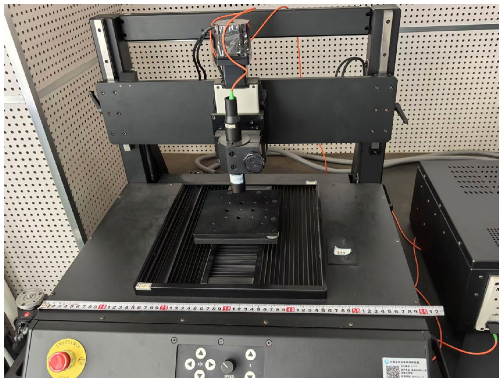
2.1.4. Wear Depth Measurements

The average wear depth of the airfoil was calculated by measuring the airfoil’s mass loss as follows:

The airfoil’s mass loss due to wear can be defined as

$$∆m=m\left(t\right)-m_0,$$

(1)

where $∆m$ is the cumulative mass loss of the airfoil (mg), $m\left(t\right)$ is the airfoil’s mass at time t (mg), and $m_0$ is the airfoil’s initial mass (mg).

The average wear depth of the airfoil can be defined as

$$∆h={\displaystyle \frac{∆m}{{\rho }_{m}S}}\times 1000,$$

(2)

$$S=l·b,$$

(3)

where $∆h$ is the cumulative wear depth (µm), ${\rho }_m$ denotes the material density of the sample (g/cm³), $S$ represents the surface area of the airfoil (mm²), $l$ denotes the arc length of the airfoil (203.9 mm), and $b$ is the airfoil’s span (30 mm).

The wear rate can be defined as

$$E={\displaystyle \frac{∆h_{ave}}{t}}$$

(4)

where $∆h_{ave}$ is the average wear depth.

2.2. Numerical Calculations

2.2.1. Three-Dimensional (3D) Model and Meshing of the Test Section

Numerical wear calculations were performed to investigate the effects of particle impact and internal flow characteristics in the near-wall region of the airfoil’s leading edge on wear and to explore the underlying wear mechanism. The flow channel’s geometry was modeled using three–dimensional modeling software, such as UG 12.0, based on the sediment abrasion tests conducted in the vane cascade, as illustrated in Figure 7. Owing to its robust adaptability, a tetrahedral unstructured mesh was used to discretize the computational domain, with mesh refinement applied in the near-wall region of the airfoil. The total number of grids (N1) was 1,264,584, and the number of nodes (N2) was 1,146,992. Figure 8 illustrates the mesh configuration.

2.2.2. Numerical Model

The Euler–Lagrange method was employed to simulate the solid–liquid two-phase flow in the flow channel, using the test conditions outlined in Section 2.1. The Eulerian method solves the time-averaged Navier–Stokes equations, whereas the Lagrangian method applies Newton’s second law to compute the particle motion. The SST k–omega (k-ω) turbulence model was selected for turbulence modeling, as it can accurately capture variations in the flow field near the wall’s surface.

The Finnie model, which is a widely accepted erosion model in the industry, as described in [21], was employed for the wear calculations. Wear is considered to be a function of the particle impact angle and velocity. Finnie’s model of erosive wear relates the rate of the wear to the rate of the kinetic energy of the impact of particles on the surface using the following functions. It distinguishes wear mechanisms through particle displacement and cutting action and is particularly suitable for wear caused by oblique impact angles. The relevant formulae are presented in Equations (5)–(7) as follows:

$$E=\mathrm{k}{V_P}^{n}f\left(\gamma \right),$$

(5)

where $E$ is the dimensionless wear parameter; $\mathrm{k}$ is a constant and depends on fluid properties, such as density, viscosity, and slurry temperature; $V_P$ denotes the particle impact velocity; and $f\left(\gamma \right)$ denotes the dimensionless function of the impact angle, defined as the angle between the particle trajectory and the wall (in radians). For common metals, $n$ typically ranges from 2.3 to 2.5; for cast iron and similar materials, $n=2$ [22].

In the numerical calculations, Equation (5) is rewritten to yield a dimensionless erosion factor as follows:

$$E={\left({\displaystyle \frac{V_p}{V_0}}\right)}^{n}f\left(\gamma \right)$$

(6)

where $V_0=\left(1/\sqrt[n]{k}\right)$; for aluminum alloys, $V_0=952 \mathrm{m}/\mathrm{s}$.

$$f\left(\gamma \right)=\left\{\begin{array}{ll}{\displaystyle \frac{1}{3}}{\cos }^2\gamma & \tan \gamma >{\displaystyle \frac{1}{3}}\\ \sin \left(2\gamma \right)-3 {\sin }^2\gamma & \tan \gamma \le {\displaystyle \frac{1}{3}}\end{array}\right.$$

(7)

Herein, $\gamma =18.42°$ is the critical value that distinguishes between sliding wear and impact wear; $\gamma <18.42°$ is predominantly sliding wear; $\gamma >18.42°$ is dominated by impact wear [22].

2.3. Calculation Methods and Boundary Conditions

The boundary parameters used in the calculations were as follows: The inlet boundary was defined as a velocity boundary (v = 8 m/s) with 5% turbulent kinetic energy. The outlet boundary is set as the outlet pressure. The flow channel’s walls and airfoil were modeled as no-slip walls with a surface roughness of 0.2 mm. The SIMPLEC algorithm was employed to solve the continuous phase, utilizing second-order schemes for the pressure, momentum, and turbulence equations. A two-way coupling approach was used to track the particle trajectories.

3. Results and Discussion

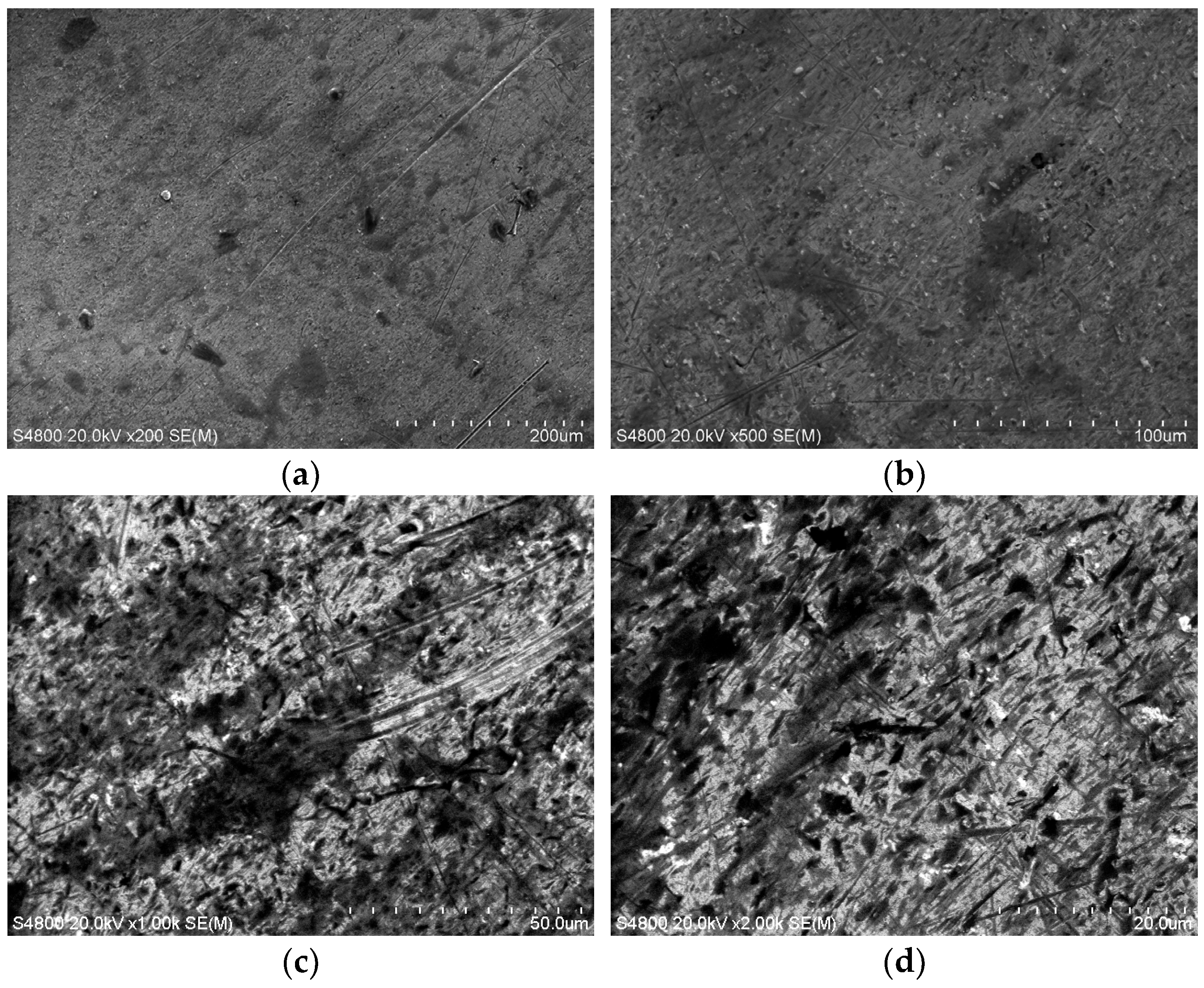
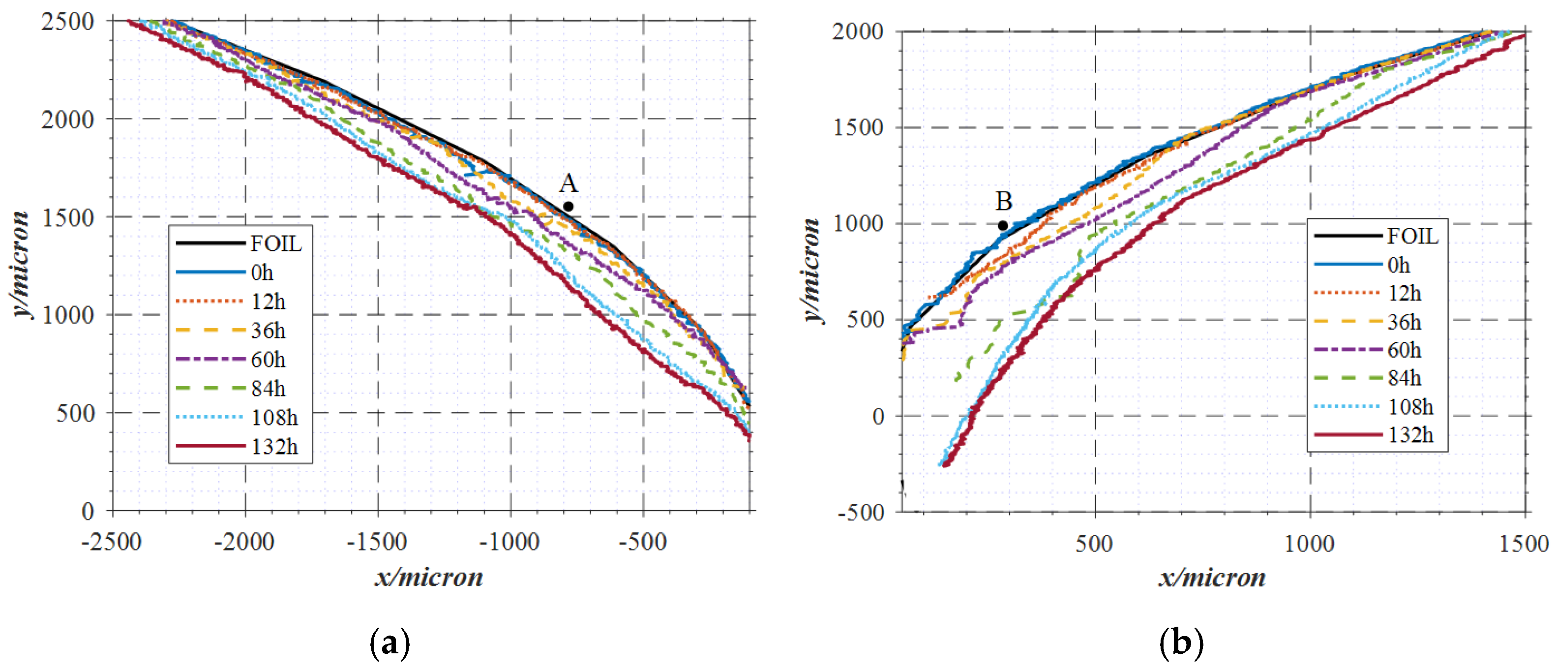
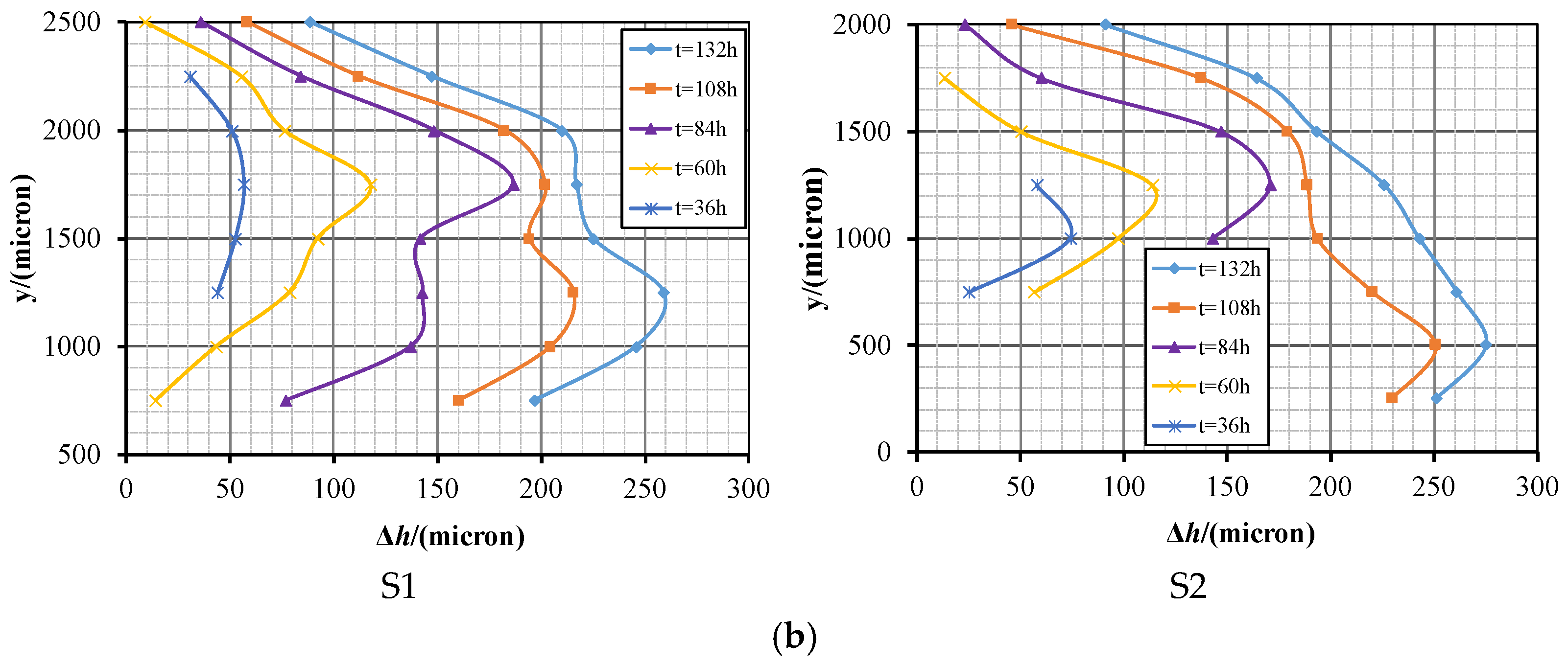
3.1. Wear Test Results and Analysis

Wear tests were performed on the airfoil using sediment-laden water at a sediment concentration of 5.61 kg/m³ to examine the wear phenomena and investigate the wear process. The test results indicated that the leading edge of the airfoil underwent the most significant wear, as shown in Figure 9.

SEM analysis was carried out to inspect the development of the erosion zone and offer valuable insights into the erosion mechanism of the leading edge of the airfoil and the path followed by the abrasive particles during the erosion process, as shown in Figure 10. Upon careful inspection of the magnified view, it becomes evident that numerous indentations are present on the surface. The scratches are oriented in diverse directions, which might be attributed to the curved configuration of the leading edge of the wing, thereby inducing the particles to impact the surface at variegated angles.

The wear process of the airfoil was analyzed by comparing the outer contour lines of the leading edge at different time intervals, as illustrated in Figure 11. From the wear trend of the leading edge over time, the wear initiation points of the S1 and S2 surfaces were A (−0.951, 1.626) and B (0.274, 0.920), respectively. The wear process can be categorized into three stages: initial (0–36 h), development (36–84 h), and stabilization (84–132 h). The wear zone expanded from the initiation points and eventually formed a wavy wear pattern, as shown in Figure 12b. At t = 36 h, a maximum wear depth value of 56.6 μm exists near the wear initiation point (A) on the S1 surface. With the accumulation of time, when t = 108 h, a waveform of “one peak and two valleys” has emerged; that is, there are two maximum wear depth values of 203 μm and 216 μm. The maximum wear depth near the wear initiation point (B) on the S2 surface is 75 μm. When t = 108 h, the two maximum wear depth values are 189 μm and 250 μm.

During the initial stage (0–36 h), the sediment-laden water impacted the airfoil’s surface, breaking through the wear initiation points and deepening the material. As shown in Figure 12 and Figure 13, after 32 h of wear accumulation, the maximum wear area width on the S1 surface increased from 0.621 mm at 12 h to 1.39 mm at 36 h (the distance between “0” and “1” in Figure 13 means the wear area width on the surface), while the wear depth increment was only 56.6 μm. The wear area width on the S2 surface increased from 0.421 mm to 0.870 mm, and the wear depth increment was 74 μm. The increments in the wear depths of the S1 and S2 surfaces are relatively small in comparison to the wear areas. Therefore, at this stage, both the wear area and depth were relatively small, and the wear area began to expand, whereas the increase in the depth remained insignificant. Overall, the wear development was slow. The maximum width of the wear area on the S1 surface was 1.39 mm, with a maximum wear depth of 56.6 μm. The S2 surface had a maximum wear area width of 0.870 mm and a maximum wear depth of 74 μm. The wear area on the S1 surface was broader than that on the S2 surface; however, the wear depth was smaller than that on the S2 surface.

Table 4. The maximum wear depths of the S1 and S2 surfaces.

Test Time t/h	Maximum Wear Depth
	S1 Surface	S2 Surface
36	56.6	74.0
60	117.8	113.8
84	186.3	170.9
108	215.5	250.7
132	258.9	275.0

lists the maximum wear depths of the S1 and S2 surfaces at different stages.

During the development stage (36–84 h), the wear area on the S1 surface continued to expand, with the maximum width increasing from 1.39 to 2.68 mm, as shown in Figure 14. The wear depth also increased, forming two core wear zones at 500 μm and 1150 μm from the leading edge, with two wear depth maxima. The second core wear zone, situated downstream, reached a maximum wear depth of 186.3 μm. On the S2 surface, the wear area expanded from 0.87 to 1.13 mm, and the wear depth gradually deepened and shifted downstream. The maximum wear depth is 170.9 μm during this stage.

During the stabilization stage (84–132 h), the wear area width on the S1 surface expanded to 3.11 mm, forming a wave-like pattern with “one peak and two valleys”. A distinct inflection point emerges between the two core wear zones. The wear rate decreased in the second core wear zone downstream from the airfoil and accelerated in the first core wear zone upstream. The wear depth gradually exceeded the second extremum, reaching a new maximum depth of 215.5 μm at 1250 μm from the leading edge. On the S2 surface, the wear zone continued to extend downstream, with the width of the wear area increasing to 1.28 mm; this expansion was less significant than that in the previous stage. The maximum wear depth increased significantly to 250.7 μm, surpassing that of the S1 surface. Figure 15 shows the wear surface contour lines for the S1 and S2 surfaces during the stabilization stage.

3.2. Numerical Simulation Results and Analysis

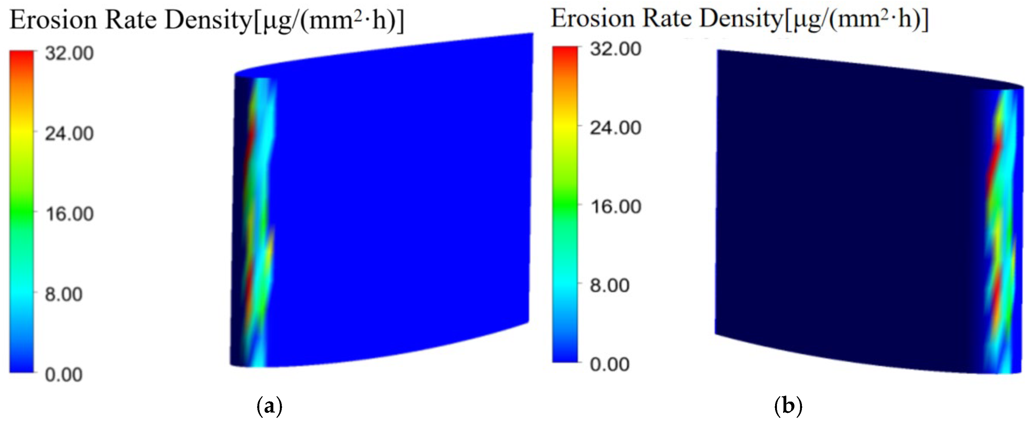
3.2.1. Comparison of Predicted Airfoil Wear Results with Test Data

The wear tests indicated that the primary wear of the airfoil occurred at the leading edge. We focused on the effect of 65.9 μm particles on the leading-edge wear of the airfoil under specific material, flow rate, and sediment concentration conditions. Therefore, the particle flow distribution in the near-wall region of the leading edge of the airfoil is a critical factor affecting the wear. In this section, the performed numerical simulations are presented to analyze the motion characteristics of particles near the leading edge before wear occurs. The numerical wear results are compared with the wear test results, as shown in Figure 16. Additionally, the wear mechanism at the leading edge of the airfoil during the initial stages of the wear tests was examined.

The wear rate density represents the mass loss of a material per unit of area per unit of time. This is a key parameter for evaluating the wear severity. From Figure 12, it can be observed that wear mainly occurred at the leading edge of the airfoil. The numerical simulation results were consistent with the wear distribution observed in the wear tests (Figure 9). Figure 17 presents the numerical simulation and wear test results for surfaces S1 and S2 at the leading edge along the horizontal plane at 50% of the airfoil’s span. The black lines depict the wear depths (∆h) at various locations from the wear test, while the red lines represent the wear rate densities (Er) at different locations from the numerical simulation. As shown in the figure, the distribution patterns of the wear rate density and wear depth are generally consistent. Along the y-axis of the leading edge of the airfoil, both the wear rate density and wear depth initially increased and then decreased, whereas on the S1 surface, it occurred at y = −1.75 mm, and on the S2 surface, it occurred at y = 1.0 mm, both corresponding to the locations of the maximum wear rate density. This confirmed the accuracy of the numerical simulations.

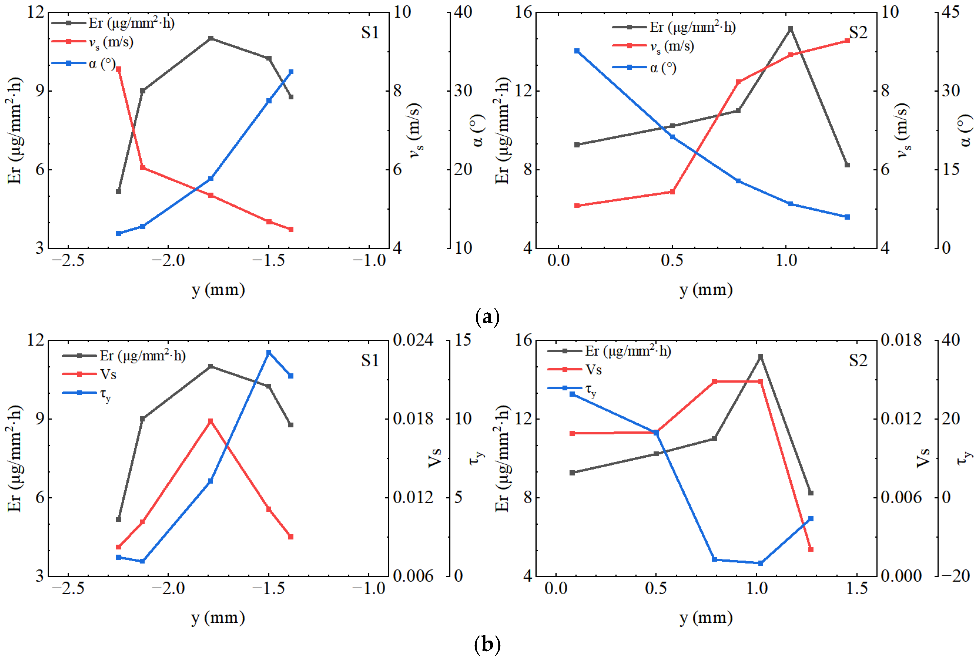
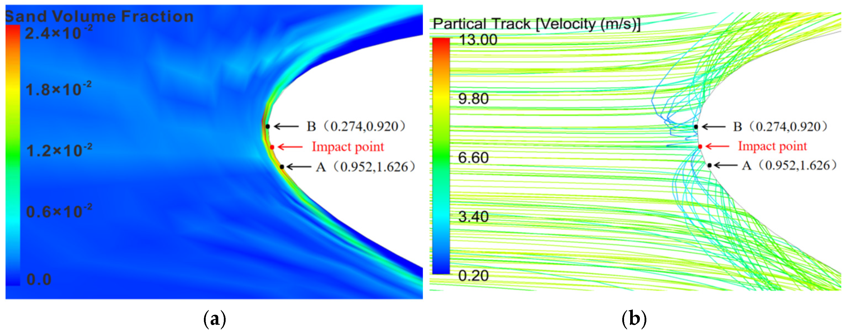
3.2.2. Airfoil’s Wear Mechanism Analysis

The wear distribution at the leading edge of the airfoil was directly related to the particle motion characteristics and particle concentration before impact. By extracting parameters, such as the solid-phase velocity, impact angle, particle volume fraction, and particle motion trajectory, in the near-wall region, the solid-phase motion characteristics were analyzed to study the wear generation mechanism at the leading edge of the airfoil. Figure 18 shows the distribution curves of the solid–liquid two-phase velocity along the y-axis in the near-wall region at the leading edge of the airfoil. Curves with the same color indicate that they are located at the same x-coordinate. The solid line with symbols represents the solid-phase velocity, whereas the dashed line represents the liquid-phase velocity. It is clear from the figure that the closer to the wall (i.e., the smaller the absolute values of x and y), the more pronounced the velocity slip is between the solid and liquid phases. A velocity minimum was observed within the range from y = −4 mm to 4 mm. Combining this with Figure 17, it can be seen that in the region between y = −2.5 mm and −1.5 mm, the impact velocity in the wear zone was relatively low. The solid phase in the near-wall region at the leading edge of the airfoil impacts the wall at a low velocity (Figure 18).

To investigate the patterns of the wear characteristics at the leading edge of the airfoil’s surfaces (S1 and S2), as well as those of the particle impact characteristics during the initial stage of the wear, data were collected from the 50% spanwise section of the airfoil, using the y-axis as the horizontal coordinate. The collected data included the wear rate densities of surfaces S1 and S2, along with the corresponding particle impact velocities, impact angles, volume fractions, and wall’s shear stresses, as shown in Figure 19. As shown in Figure 19, the wear patterns on surfaces S1 and S2 are mostly consistent. Along the y-axis, moving toward the leading edge, the wear rate density initially increased and then decreased, reaching peak values at y = −1.79 mm and y = 1.02 mm. The maximum wear rate density of S2 was higher than that of S1. As shown in Figure 19a, the wear rate density did not have a direct positive correlation with the particle impact velocity or the impact angle. Moving closer to the leading edge along the y-axis, the impact velocity tended to decrease, whereas the impact angle increased. From Figure 19b, it is clear that the particle volume fraction is not positively correlated with the wear rate density.

The highest wear rate density occurred at the point of the maximum particle volume fraction. For the wall’s shear stress, Figure 19b shows that the shear stress in the y-direction influenced the wear rate density. Positive stress acts on surface S1, whereas negative stress affects surface S2. The maximum shear stress point on surface S2 coincides with the maximum wear rate density and particle volume fraction, whereas the maximum stress point on surface S1 does not coincide with the maximum wear rate density. This indicates that the particle volume fraction has a greater impact on the wear rate than the shear stress in the y-direction. The higher wear rate density on surface S2 was because of the higher particle volume fraction compared with that on surface S1.

Figure 20 shows the distributions of the particle volume fraction and particle motion trajectories at the leading edge of the airfoil in a 50% spanwise section. As shown in Figure 20a, there were particle accumulation zones near the wall on both the S1 and S2 surfaces at the leading edge of the airfoil. This was mainly caused by the particles impacting the wall at high impact angles, rebounding, and secondary impacts on the downstream wall. Therefore, two points of initial wear, A (0.952, 1.626) and B (0.274, 0.920), appeared during the initial wear stage. The different coordinates of points A and B were owing to the asymmetric nature of the incoming flow. From the particle trajectory in Figure 20b, it can be observed that flow separation occurred downstream from the leading edge of the airfoil, which was the main reason why the wear was concentrated at the leading edge.

The results of the model test and numerical simulation for sediment abrasion show a relatively high degree of consistency. On the 50% wingspan measurement surface, the wear depth obtained from the experiment is essentially in correspondence with the wear rate density from the numerical simulation. Based on the model test and numerical calculation results, the mechanism of the sediment abrasion is summarized as follows: The wear at the leading edge of the airfoil was influenced by several factors, including the particle impact velocity, impact angle, particle volume fraction, and shear stress in the y-direction. The wear mostly occurred at the leading edge of the airfoil, mostly because of the flow separation in the downstream region of the leading edge. A low-velocity zone was identified near the impact point at the airfoil’s leading edge, where the particles impacted the wall at relatively low velocities and high impact angles. After the initial impact, the particles rebounded and caused a secondary impact downstream from the initial impact point, leading to a number of particles accumulating near points A and B. Therefore, in the initial stage of the wear, the initiation points of the wear are at points A and B, which deviate downstream from the impact points. Because of the asymmetric incoming flow, the wall’s shear stress in the y-direction near point B on the S2 surface is greater than that near point A on the S1 surface. Consequently, the maximum wear depth and the maximum wear rate density of the S2 surface are higher than those of the S1 surface.

4. Conclusions

This study investigated leading-edge wear on an airfoil in sediment-laden water, using tests and numerical simulations. The wear development process was analyzed experimentally, and numerical simulations were employed to investigate variations in the wear rate density, particle flow field characteristics, and particle impact characteristics during the initial wear stage. This approach enhances our understanding of the mechanisms that affect the leading edge of an airfoil.

The following conclusions were drawn from the wear tests:

Based on the physical testing, the wear process was categorized into three stages: the initial (0–36 h), development (36–84 h), and stabilization stages (84–132 h). During the initial stage, both surfaces S1 and S2 exhibited extreme points of wear depth, with the wear depth profile approximating a parabolic curve. The maximum wear depth on the S1 surface was smaller than that on the S2 surface.

During the development stage, two wear-depth maxima appeared on the S1 surface. The wear depth in the previous stage continued to increase. A second extreme point emerged, and the maximum wear depth on the S2 surface progressively increased, shifting downstream along the airfoil’s surface. The maximum wear depth of the S1 surface exceeded that of the S2 surface.

During the stabilization stage, compared to the previous stage, the wear rate at the first extreme point on the S1 surface decreased, whereas the wear rate at the second extreme point increased, with the wear depth surpassing that at the first extreme point. The deepest wear point shifted further downstream, and, ultimately, the maximum wear depth on the S1 surface was less than that on the S2 surface.

The following conclusions can be drawn from the numerical simulations:

During the initial stage, the wear rate density is primarily influenced by the particle impact velocity, impact angle, particle volume fraction, and shear stress in the y-direction. A low-velocity zone exists near the impact point, where particles, after impacting the wall at a relatively low velocity and a high impact angle, rebound and cause secondary impacts on the downstream wall. This results in particle accumulation downstream from the impact point, creating two wear initiation points at A and B. The y-direction wall’s shear stress significantly affected the wear rate density, which explains why the maximum wear rate density on the S2 surface was higher than that on the S1 surface during the initial wear stage.

The flow separation downstream from the leading edge of the airfoil was the primary reason for the predominant wear observed at this location.

References

1. Lu, L.; Liu, J.; Yi, Y.L. Evaluation of sand abration of hydraulic in Baihetan hydropower Station. J. Hydropower 2016, 35, 67–74. (In Chinese) [Google Scholar]
2. Padhy, M.K.; Saini, R.P. Effect of Size and Concentration of Silt Particles on Erosion of Pelton Turbine Buckets. Energy 2009, 34, 1477–1483. [Google Scholar] [CrossRef]
3. Han, L.; Wang, Y.; Zhang, G.F.; Wei, X.Z. The Particle Induced Energy Loss Mechanism of Pelton Turbine. Renew. Energy 2021, 173, 237–248. [Google Scholar] [CrossRef]
4. Ge, X.; Sun, J.; Zhou, Y.; Cai, J.; Zhang, H.; Zhang, L.; Ding, M.; Deng, C.; Binama, M.; Zheng, Y. Experimental and Numerical Studies on Opening and Velocity Influence on Sediment Erosion of Pelton Turbine Buckets. Renew. Energy 2021, 173, 1040–1056. [Google Scholar] [CrossRef]
5. Zhang, G.; Wei, X.Z.; Liu, W.J. Numerical Investigation of Two-Phase Flow in the Guide Vanes Area of a Hydraulic Turbine. J. Large Electr. Mach. Hydraul. Turbine 2015, 2, 42–45. (In Chinese) [Google Scholar]
6. Chen, Y.; Li, R.; Han, W.; Guo, T.; Su, M.; Wei, S. Sediment erosion characteristics and mechanism on guide vane end-clearance of hydro turbine. Appl. Sci. 2019, 9, 4137. [Google Scholar] [CrossRef]
7. Han, W.; Chen, Y.; Li, R.; Su, M.; Peng, G.; Wei, S. Sediment-wear morphology prediction method of hydraulic machine based on differential-quadrature method. Mod. Phys. Lett. B 2019, 33, 1950172. [Google Scholar] [CrossRef]
8. Rakibuzzaman, M.; Kim, H.H.; Kim, K.; Suh, S.H.; Kim, K.Y. Numerical study of sediment erosion analysis in Francis turbine. Sustainability 2019, 11, 1423. [Google Scholar] [CrossRef]
9. Jia, L.; Zeng, Y.; Liu, X.; Huang, W. Numerical Simulation and Experimental Study on Sediment Wear of Fixed Guide Vanes of Hydraulic Turbines in Muddy River Based on Discrete Phase Model. Processes 2023, 11, 2117. [Google Scholar] [CrossRef]
10. Chen, M.; Tan, L.; Fan, H.; Wang, C.; Liu, D. Solid-liquid multiphase flow and erosion characteristics of a centrifugal pump in the energy storage pump station. J. Energy Storage 2022, 56, 105916. [Google Scholar] [CrossRef]
11. Shrestha, U.; Chen, Z.; Choi, D.Y. Correlation of the Sediment Properties and Erosion in Francis Hydro Turbine Runner. Int. J. Fluid Mach. Syst. 2019, 12, 109–118. [Google Scholar] [CrossRef]
12. Zhang, L.; Cao, Z.Y.; Wang, J.L. Research on the Influence of Operating Conditions on the Abrasion in the Guide Vane Area of Turbines in Multi-Sand Rivers. Water Resour. Hydropower Eng. 2022, 53, 148–156. (In Chinese) [Google Scholar]
13. Thapa, S.B.; Trivedi, C.; Dahlhaug, G.O. Design and Development of Guide Vane Cascade for a Low Speed Number Francis Turbine. J. Hydrodyn. 2016, 28, 676–689. [Google Scholar] [CrossRef]
14. Koirala, R.; Neopane, H.P.; Zhu, B.; Thapa, B. Effect of sediment erosion on flow around guide vanes of Francis turbine. Renew. Energy 2019, 136, 1022–1027. [Google Scholar] [CrossRef]
15. Brekke, H.; Wu, Y.L.; Cai, B.Y. Design of Hydraulic Machinery Working in Sand Laden Water, 2nd ed.; Imperial College Press: London, UK, 2002; Volume 2, pp. 155–181. [Google Scholar]
16. Song, X.; Zhou, X.; Song, H.; Deng, J.; Wang, Z. Study on the Effect of the Guide Vane Opening on the Band Clearance Sediment Erosion in a Francis Turbine. J. Mar. Sci. Eng. 2022, 10, 1396. [Google Scholar] [CrossRef]
17. Yao, B.; Li, J.; Zhao, T.; Liu, X. Sediment wear prediction model of ZG06Cr13Ni4Mo turbine guide vane in sediment-laden hydropower station. Mater. Express 2021, 11, 1866–1873. [Google Scholar] [CrossRef]
18. Zhao, X.; Peng, Y.; Yang, J.; Chen, J.; Xu, L.; Tang, W.; Liu, X. Sediment wear of turbine guide vane before and after tungsten carbide treatment. Adv. Mech. Eng. 2022, 14, 1–16. [Google Scholar] [CrossRef]
19. Thapa, S.B.; Dahlhaug, G.O.; Thapa, B. Effects of sediment erosion in guide vanes of Francis turbine. Wear 2017, 390–391, 104–112. [Google Scholar] [CrossRef]
20. Zhu, L.; Zhang, H.; Chen, Y.; Meng, X.; Lu, L. Asymmetric Solid–Liquid Two-Phase Flow Around a NACA0012 Cascade in Sediment-Laden Flow. Symmetry 2022, 14, 540. [Google Scholar] [CrossRef]
21. Dosanjh, S.; Humphrey, J.A. The influence of turbulence on erosion by a particle-laden fluid jet. Wear 1985, 102, 309–330. [Google Scholar] [CrossRef]
22. Noon, A.A.; Kim, M.H. Erosion wear on centrifugal pump casing due to slurry flow. Wear 2016, 364, 103–111. [Google Scholar] [CrossRef]
Figure 1. Structure of the Venturi abrasion test system.
Processes 12 02790 g001
Figure 2. Venturi abrasion test setup.
Processes 12 02790 g002
Figure 3. The experimental section part.
Processes 12 02790 g003
Figure 4. Channel’s dimensions in the test section.
Processes 12 02790 g004
Figure 5. Surface profiler.
Processes 12 02790 g005
Figure 6. Morphological data acquisition and processing.
Processes 12 02790 g006
Figure 7. Three-dimensional (3D) model of the test section.
Processes 12 02790 g007
Figure 8. Mesh division schematic.
Processes 12 02790 g008
Figure 9. Wear test results: (a) airfoil wear; (b) S1 surface wear; (c) S2 surface wear.
Processes 12 02790 g009
Figure 10. Morphology of the leading edge of the airfoil after sediment erosion at different scales: (a) 200 μm; (b) 100 μm; (c) 50 μm; (d) 20 μm.
Processes 12 02790 g010
Figure 11. Outer contour lines of the leading edge at different time points for the S1 and S2 surfaces: (a) S1; (b) S2.
Processes 12 02790 g011
Figure 12. Wear depth at the leading edge of the airfoil: (a) depth measurement points; (b) depth profile.
Processes 12 02790 g012aProcesses 12 02790 g012b
Figure 13. Wear processes of S1 and S2 surfaces of the airfoil’s leading edge during the initial stage: (a) S1 surface; (b) S2 surface.
Processes 12 02790 g013
Figure 14. Wear processes of S1 and S2 surfaces of the airfoil’s leading edge during the development stage: (a) S1 surface; (b) S2 surface.
Processes 12 02790 g014
Figure 15. Wear processes of S1 and S2 surfaces of the airfoil’s leading edge during the stabilization stage: (a) S1 surface; (b) S2 surface.
Processes 12 02790 g015
Figure 16. Wear rate density distributions: (a) wear rate density on the S1 surface; (b) wear rate density on the S2 surface.
Processes 12 02790 g016
Figure 17. Comparison of numerical simulation and wear test results: (a) S1 surface; (b) S2 surface.
Processes 12 02790 g017
Figure 18. Solid–liquid two–phase velocity distribution curves in the near-wall region at the leading edge of the airfoil (Re = 8.0 × 10⁵): (a) Upstream zone; (b) Near wall zone.
Processes 12 02790 g018
Figure 19. Wear at the leading edge of the airfoil. (a) Wear rate density versus particle velocity and impact angle. (b) Wear rate density vs. particle volume fraction and wall’s shear stress.
Processes 12 02790 g019
Figure 20. Particle volume fraction and motion trajectories in the near-wall region at the leading edge of the airfoil: (a) particle volume fraction; (b) particle trajectories.
Processes 12 02790 g020