General Methodology for Laser Welding Finite Element Model Calibration

Abstract

Laser welding has become increasingly popular in recent decades due to its high processing speed and minimal heat-affected zone, which contribute to extended component lifetimes. However, the adoption of this advanced technique is often hindered by a lack of skilled personnel associated with traditional welding and limited awareness of its potential. This study proposes a straightforward methodology for developing a finite element-based thermal model for laser welding, incorporating a two-step experimental calibration process. Using temperature measurements from thermocouples and data from a welding spot test, the numerical model was calibrated to optimize combinations of welding speed and power. The study focuses on S275JR structural steel, involving initial spot weld followed by a linear welding trajectory. The results demonstrate the precision of the proposed calibration approach, as numerical predictions closely align with experimental data from all three thermocouples. The findings validate the effectiveness and accuracy of this methodology, highlighting its ability to adapt spot calibration results to more complex linear welding scenarios. Moreover, the simplicity of the process ensures it is accessible and broadly applicable across different materials and welding configurations. This work offers a reliable and resource-efficient framework for laser welding process optimization in industrial applications.

1. Introduction

Traditionally, structural steels, such as S275 and S355, have been joined using arc welding technology in the construction of bridges, heavy machinery, wind turbines, and numerous other structures [1]. Although arc welding is a well-established and reliable joining method, it presents certain limitations and challenges that can result in significant economic losses for manufacturers globally.

One of the primary challenges associated with high-energy welding processes is distortion, which can lead to misalignments or even cracking. These issues arise from the substantial heat input involved in welding, which not only melts the filler material, but also partially fuses the base material, significantly affecting its microstructure. The heat-affected zone (HAZ) may undergo phase transformations, altering the internal structure of the material and consequently its mechanical properties [2,3]. Furthermore, the thermal expansion and subsequent contraction of the heated metal induce substantial residual stresses within the workpiece. Often, post-weld treatments or additional adjustments are required to correct distortions, align the components, or facilitate further assembly operations. The combination of residual stresses and those introduced during corrective adjustments can significantly reduce the fatigue resistance of the structure, ultimately compromising its service life [4].

Given the limitations of traditional welding methods, recent studies have explored the potential of replacing arc welding with laser welding with filler material for structural components subjected to cyclic loading [5]. While the initial cost of the equipment is higher, laser welding offers a more concentrated heat input, which reduces the size of the heat-affected zone (HAZ) and lowers the overall thermal input. This distinction leads to a reduction in thermal distortions, mitigates residual stresses, and minimizes the need for post-weld adjustments, thereby enhancing the fatigue resistance and extending the service life of the structure [6,7]. Additionally, laser welding enables the joining of thinner plates and materials that are less commonly welded, such as aluminum, titanium, and even plastics [8,9].

Additionally, due to the general lack of skilled labor and the abrupt decrease in laser welding equipment price in the last years, the usage of laser welding in the industry is forecasted to highly increase and be a game-changer in the coming years, with a special impact on structural welding industries [10,11]. However, the introduction of this new technology may present challenges for process engineers, as transitioning from arc welding to laser welding requires the calibration of new variables, a comprehensive understanding of the process, and an in-depth analysis of how various parameters affect weld quality. Nevertheless, this new technology is easier to comprehend and master from the perspective of process engineers, thereby facilitating its industrial adoption. Consequently, the current demand for skilled arc welders would be significantly reduced. Plant workers would not require extensive expertise in the field, as the responsibility for determining the appropriate process variables at any given time would rest with the process engineer.

One key challenge in laser welding is the implementation of this new technology, as it functions different to traditional arc welding. Thus, it requires many attempts to learn how to operate the machine and to be able to set the optimal parameters for each process.

To streamline this intensive iterative task, simulation models are developed to calculate the effects of numerous variables within significantly shorter timeframes. This virtual experimentation strategy is widely employed across various fields, including medicine [12], electronics [13], and climatology [14], among others. However, in the context of laser welding simulations, most studies focus on process-specific phenomena and conduct highly detailed investigations [15,16,17].

As a result, there is a notable lack of straightforward, easily replicable simulations, efficient problem-solving tools, and economically accessible software in this field. To address these gaps, this article primarily introduces a comprehensive and simplified guide for developing a thermal finite element-based numerical model for laser welding. The proposed model is grounded in a two-step experimental calibration methodology. Its validity is demonstrated through experimental data, and its applicability to a broad spectrum of laser welding equipment is thoroughly evaluated. The proposed methodology aims to streamline the integration of laser welding systems by focusing on the calibration of the laser source via numerical modeling. By using a thermocouple and a welding spot, a numerical simulation can be developed and calibrated. Upon completion of the model, laser welding parameters, such as speed and power, can be easily optimized. Furthermore, a change in material would only necessitate a new experimental test and the corresponding adjustment of model parameters.

2. Methodology

This methodology can be approached from two distinct perspectives, as illustrated in Figure 1. First, the experimental setup may be implemented as an initial step, followed by the development of the numerical model once sufficient data have been collected. Alternatively, a numerical model can be created upfront, with gaps left to be filled by the experimental data. Additionally, both approaches can be pursued concurrently if efficiency is a priority. While both methods are expected to yield successful results, step-by-step progression is recommended, starting with the experimental setup, as outlined in this article.

Firstly, the selection of the welding material must be made, along with the definition of the welding parameters. While most parameters may be appropriate, the critical aspect lies in comprehending these parameters and accurately determining their respective values. Similarly, while the material’s properties play a vital role in the simulation process, they are comparatively less significant during the experimental phase. The most efficient approach is to use a spot configuration, where the welding speed is set to zero. This reduces the number of variables and simplifies the manual calibration process.

After selecting the material and defining the welding parameters, a data acquisition system must be implemented. The simplest setup consists of a thermocouple paired with an appropriate data reader.

Next, a short weld spot is applied as close as possible to the thermocouple without directly irradiating it, to prevent damage to the junction between the sensor and the material. The distance from the center of the weld spot to the center of the thermocouple must be precisely measured, as this distance is critical for ensuring accurate simulation results. This procedure can be repeated multiple times, targeting different areas around the thermocouple. By doing so, the results can be compared to identify any anomalies in the data acquisition process.

Once the data are recorded, a numerical model must be developed. The process of developing the model involves three key steps, in addition to replicating the material geometry used in the experimental setup: spot size calculation, meshing, and material modeling.

Regarding the spot size calculation, the beam size profile and spot size at the focal point are typically not provided by the equipment manufacturer. However, by integrating specific characteristics of the laser welding machine with relevant equations, it becomes possible to calculate the beam profile and spot size at the focal point, as elaborated later in the document.

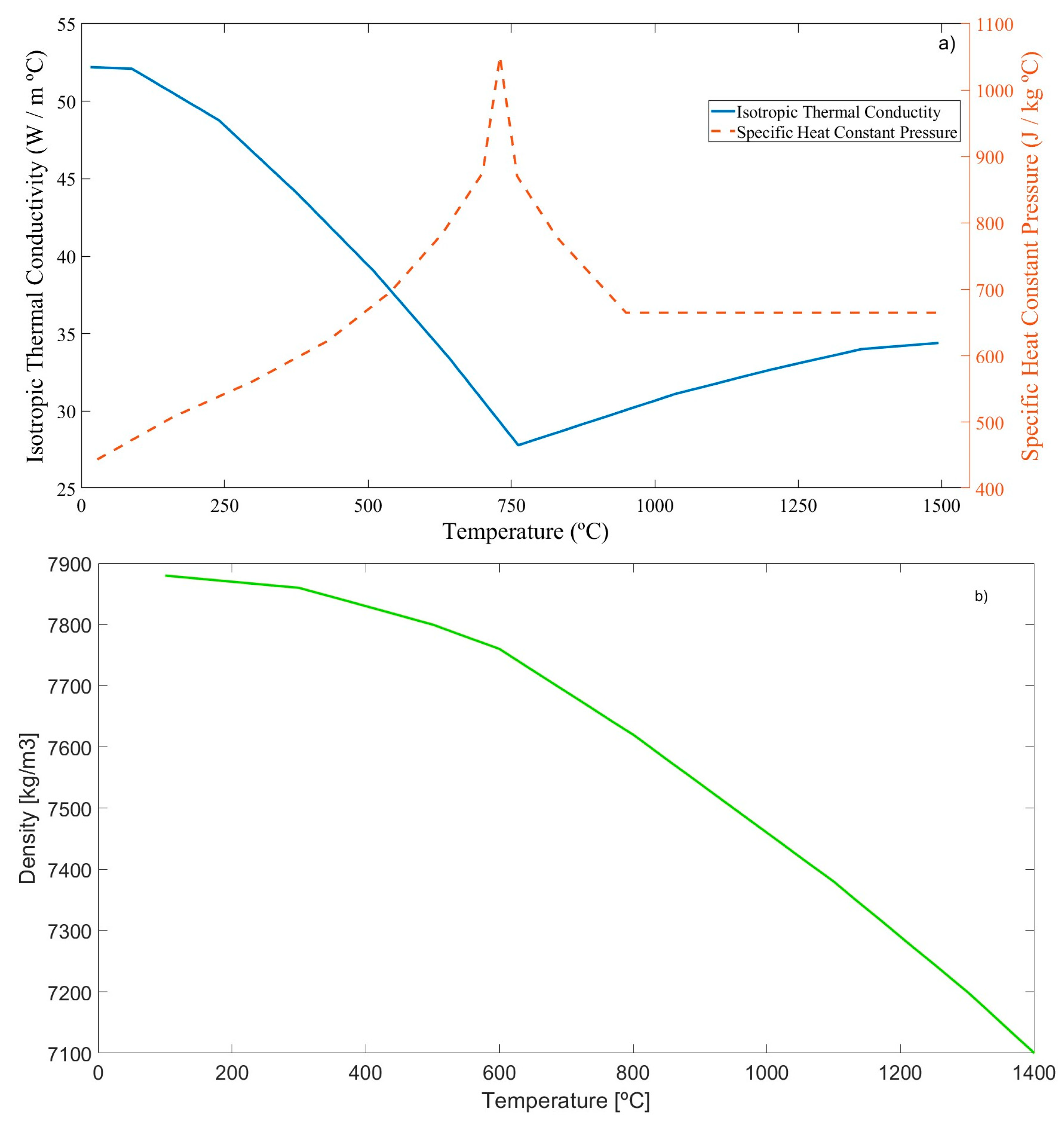
The material model requires data on specific heat at a constant pressure, isotropic thermal conductivity, and temperature-dependent density. For most materials, these properties are readily available from online sources, unless a particularly rare material is being used.

Finally, by combining all the preceding steps, the absorptivity value is calibrated using a reverse engineering approach until the simulated curve closely matches the experimental data.

In this article, a second weld case was developed, both experimentally and numerically, to verify the results and to validate the methodology.

2.1. Case Study and Equipment

The case study presented in this project focuses on two S275JR steel plates: a 30 mm × 30 mm × 3 mm square plate for spot calibration, and a 150 mm × 100 mm × 3 mm rectangular plate for linear model validation. S275JR was chosen due to its widespread use in structural construction and its broad range of applications.

The equipment used in this study was a water-cooled, handheld MFSC 1500X-SUP20S fiber laser welding machine. The laser source, provided by MAX Photonics (Gujarat, India), emits a laser beam with a maximum power of 1500 W and a wavelength of 1080 nm. In addition to the intrinsic focal length of the mirror array, manual adjustment is possible within a range of ±10 mm. Although the system primarily operates with a continuous beam, it also offers a linear oscillation capability of up to 6 mm at a maximum oscillation frequency of 5000 Hz. Details of the selected laser equipment are provided in

Table 1. MFSC 1500X-SUP20S laser welding machine parameters [18].

Parameter	Value
Laser power	100–1500 W
Wavelength	1080 nm (±10 nm)
Collimating lens	D20 × 5/F60
Focal lens	D20 × 4.5/F150
Spot oscillation range	0–6 mm
Diameter of laser fiber	50 µm

.

3. Laser Source Calibration

3.1. Calibration Experimental Setup

The experimental setup was divided into two main phases. The first phase focused on calibrating the laser welding source, while the second phase was dedicated to generating experimental data to feed the simulation and enhance its accuracy.

An array of three K-type thermocouples was employed to measure the temperature during both the laser source calibration and the numerical model validation phases. The thermocouples were connected to a National Instruments NI 9235 signal conditioning module, which interfaced with an NI eDAQ-9178 data acquisition device that communicated with a laptop. A custom temperature-monitoring and data-recording program, developed in LabVIEW 2014 (Emerson Electric Co., St. Louis, MO, USA), was used to log the acquired data.

For safety reasons, the laser equipment operated with a trapezoidal power profile, as illustrated in Figure 2. Consequently, the laser source did not immediately reach the maximum selected output power, nor was it abruptly turned off. Instead, a minimum power value was specified for both the initial and final stages of operation. In this case, for a welding sequence with an output power of 1000 W, the minimum power was set to 300 W. The ‘Laser on Progressive Time’ was set to 200 ms, while the ‘Laser Off Progressive Time’ was set to 300 ms.

Since laser welding produces a relatively small heat-affected zone (HAZ), it is crucial to position the welding spot as close as possible to the thermocouples. Otherwise, it may be challenging to detect a significant temperature gradient. To aid in the subsequent development of the numerical model, it is advisable to measure and mark the location of each welding spot after the process. In this case, the distance between the thermocouple and the center of the welding spot was set to 4 mm.

3.2. Heat Source Model

Once all the data are processed, a finite element model must be created. The general form of the three-dimensional heat conduction Equation (1) was solved by means of the finite element method. This equation requires some material properties such as conduction coefficient ($\lambda$), density (ρ), energy rate generation per unit volume of the medium, and specific heat at a constant pressure ${(C}_p$).

$${\displaystyle \frac{\partial }{{\partial }_x}}\left(\lambda {\displaystyle \frac{\partial T}{\partial \mathrm{x}}}\right)+{\displaystyle \frac{\partial }{{\partial }_y}}\left(\lambda {\displaystyle \frac{\partial T}{\partial y}}\right)+{\displaystyle \frac{\partial }{{\partial }_z}}\left(\lambda {\displaystyle \frac{\partial T}{\partial z}}\right)+q_v=\mathsf{\rho }{c}_p{\displaystyle \frac{\partial T}{\partial t}}$$

(1)

Due to its more concentrated energy distribution, laser welding is typically modeled using a Gaussian distribution heat source model. Depending on the application, two variations can be considered: conduction welding and keyhole welding. Keyhole welding is generally applicable in cases where the laser penetrates the material, such as in lap welding. In contrast, conduction welding is used when filler material is required or when penetration is not achieved due to process dynamics. This type of welding is commonly employed in butt welding with filler material.

In this case, the most representative welding method is conduction welding, best recreated by the superficial Gaussian heat distribution. Thus, assuming the beam is completely focused on the spot, the beam radius (r_e) is 100 µm and the maximum heat value (Q₀) was stablished at 1000 W (see Figure 3).

The Gaussian Equation (2) was extracted from [19].

$$Q_f\left(x,y,z\right)=Q_0·e^{\left(-{\displaystyle \frac{x^2+y^2}{{r_e}^2}}\right)}$$

(2)

The calculation of the spot size is based on the work of Rüdiger [20] and the parameters of the selected laser equipment are provided in Table 1.

Table 2. Spot size calculation parameters.

Parameter	Value
BPP	1.5 m/mrad
M2	4.43
Divergence half-angle (Θ)	0.339 mrad
Rayleigh length (z0)	6.67 mm

shows the calculated parameters related to the spot size.

Once the parameters are obtained via Equation (3), the Gaussian beam radius profile can be calculated, as shown in Figure 4, where the beam radius at the focal point can be observed.

$$w\left(z\right)=w_0\sqrt{1+{\left(M^2{\displaystyle \frac{z}{z_R}}\right)}^2}$$

(3)

3.3. Calibration Numerical Model

A numerical model was developed using ANSYS R22b software (Ansys Iberia S.L., Madrid, Spain), with several simplifying assumptions. First, the dimensions were directly obtained from the experimental probe, resulting in a piece with dimensions of 30 mm × 30 mm × 3 mm. Second, phase transformations and latent heat effects were excluded from the model. Lastly, all surfaces were assigned a convective heat transfer coefficient of 5 W/m²·K and a radiation emissivity of 0.9, simulating a controlled environment with no air movement. An ambient temperature of 25 °C was assumed, as the welding process typically heats the room in which it is conducted.

Meshing is a critical step in any numerical simulation, although in this case, it is relatively simple. The minimum element size must be at least twice as small as the spot size at the focal point to ensure the system has sufficient resolution to accurately capture the evolution of the welding spot. Consequently, a mesh with a general element size of 50 µm was generated. As shown in Figure 5, a mesh composed of 172,800 eight-node hexaedral elements (SOLID278) was used, as linear elements provide equivalent results to quadratic elements but with a lower computational cost.

The acquisition system obtains a new input once every 100 ms; thus, the time step for the simulation was set to 100 ms. The moving heat source model was implemented using APDL (Ansys Parametric Design Language).

3.4. Material Model

As mentioned in the Section 2.1, the chosen material was the structural steel S275JR. The density and Poisson’s ratio were obtained from Eurocode 3, in accordance with EN 1993-1-1:2005+AC2:2009 [21]. The remaining material properties were sourced from the work of Liang et al. [22]. However, only the thermal isotropic conductivity, specific heat at a constant pressure, and density are considered temperature-dependent, as illustrated in Figure 6. Other properties, such as the thermal expansion coefficient and Young’s modulus, are not used in the thermal calculations and were, therefore, not included in the model.

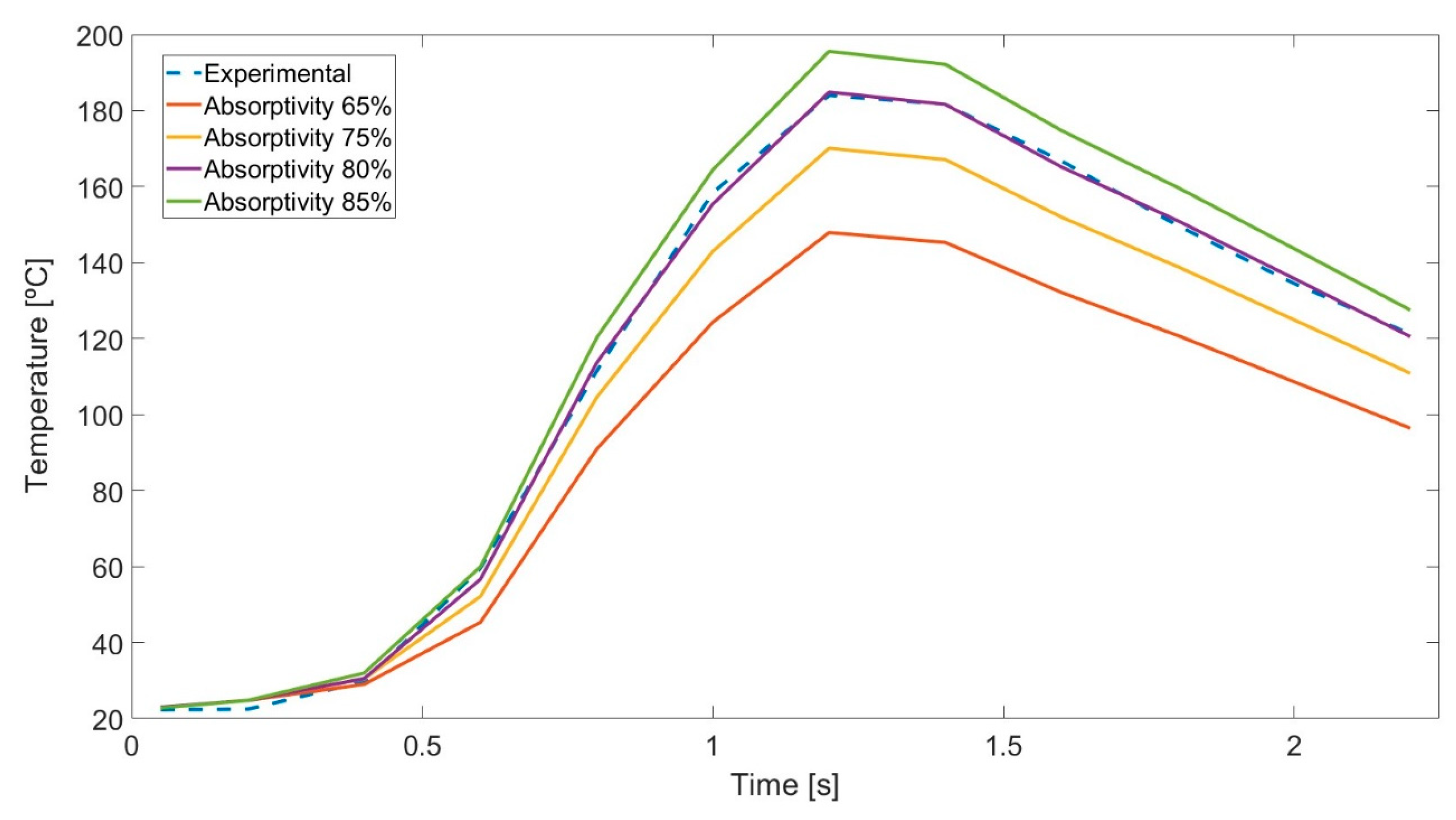
3.5. Material’s Absorptivity Calibration

An important but unknown coefficient is the absorptivity, or absorption coefficient, which represents the ability of a material to absorb incident light. The absorptivity of a material varies depending on factors such as surface finish and the wavelength of the laser beam [23]. For untreated structural steels, the absorptivity for a near-infrared laser typically ranges between 55% and 70% [24].

For the initial simulation, an absorptivity value of 65% was selected. Employing a reverse engineering approach, the experimental and numerical data were compared post-simulation. The absorptivity value was iteratively adjusted through successive simulations until a close correlation between the two datasets was achieved. In this case, the absorptivity was initially increased by 10% until the experimental data were exceeded at 85%. Subsequently, an intermediate value of 80% was found to provide the best fit, as shown in Figure 7.

4. Laser Welding Model

Once the calibration model is properly tuned, it can be applied to develop a more complex welding model. For this study, a straight welding trajectory was chosen, and this model was experimentally validated.

4.1. Experimental Validation Setup

Tooling was designed to secure the 150 mm × 100 mm × 3 mm plate to the workbench, constructed from a combination of steel plates and clamps to prevent any displacement during the welding process. A straight weld bead was then made in a single pass, at a constant speed and in one direction, using a KUKA KR 300 R2500 robotic arm (KUKA Roboter GmbH, Ausburg, Germany), which was integrated with the manual welding equipment, as shown in Figure 8. The robotic arm was utilized to ensure the precision of the weld path and maintain a consistent welding speed, eliminating the need for filler material. Custom tooling was designed and fabricated to securely mount the handheld welding device onto the robotic arm. Welding was carried out at an ambient temperature of 25 °C, with no preheating applied.

Thermocouples were welded 30 mm apart from each other and 7 mm away from the center of the seam. An additional thermocouple was positioned 10 mm away from the center. While it is important to position the thermocouples as close to the seam as possible, they must not be directly exposed to the laser or have their welded spots melted. A schematic representation of the welding seam and thermocouple positions is shown in Figure 9.

4.2. Numerical Model

Once the laser source and material are calibrated, a laser welding numerical model can be developed. The power profile used during the calibration phase will be maintained. A low welding speed of 10 mm/s was chosen to ensure adequate temperature readings from the thermocouples, although this speed is more commonly used for processes involving thicker plates [25].

The Gaussian heat source model used in the calibration step was applied, as this model is intrinsic to the welding process. Additionally, the material models remained unchanged, as they are determined by the properties of the metal. For the mesh, HEX8 (SOLID278) elements with a size of 1 mm were used. A center-concentrated bias with a factor of 50 was applied to the long edges, while a standard edge sizing was used for the short edges. This approach ensures a refined mesh near the seam, with the element size gradually increasing as the distance from the center increases. In total, 15,200 elements and 30,906 nodes were generated, as shown in Figure 10.

Similar to the calibration model, phase transformations and latent heat effects are not considered. Uniform convection and radiation coefficients are applied to all surfaces. The time step was set to 100 ms. The APDL command was modified to enable the Gaussian heat source to move across the base material.

5. Results and Discussion

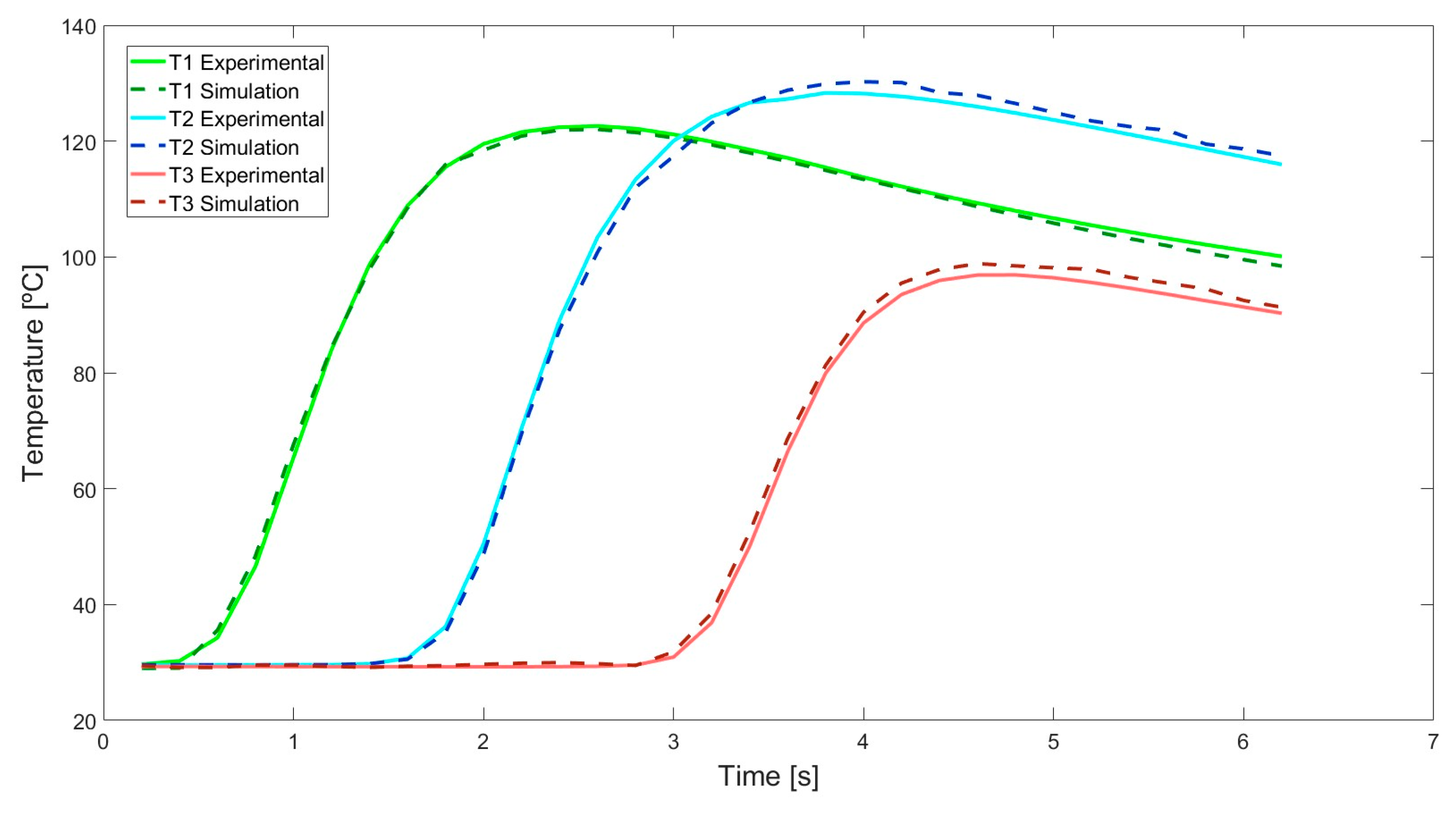
This section analyzes the results of the comparison between the numerical simulation model and the experimental data, focusing on the temperature evolution measured by three thermocouples. Figure 11 demonstrates a strong agreement between experimental and simulated temperature profiles, with a maximum error of 3%. This close correlation indicates that the simulation effectively captures the primary thermal dynamics of the system.

The first and second thermocouples exhibited similar peak temperatures, reaching approximately 128 °C and 132 °C, respectively. The temperature evolution curves exhibited a high degree of similarity, particularly during the heating phases. However, minor discrepancies are observed in the peak temperature and cooling profiles. These differences arise from the positioning of the thermocouples relative to the heat source. The first thermocouple accumulated less thermal energy prior to being reached by the laser, as the heat source travels a shorter distance, resulting in a marginally higher cooling rate compared to the second thermocouple.

In contrast, the third thermocouple displayed a notably shallower heating slope and a lower peak temperature. This behavior can be attributed to its greater distance from the heat source, which delays its heating and reduces the energy input it receives. Despite these differences, the numerical model provides a reliable approximation of the experimental behavior, particularly in the early and steady-state phases of the temperature profiles.

The results highlight the capability of the simulation to replicate the experimental data accurately while also revealing areas where further refinement may be beneficial. Addressing the observed discrepancies—potentially by incorporating additional physical effects, improving parameter calibration, or accounting for spatial heat transfer variations—could enhance the predictive accuracy of the model. Nonetheless, the agreement between experimental and simulated results demonstrates the robustness of the current modeling approach.

6. Conclusions

A straightforward methodology for calibrating a laser heat source for numerical modeling was developed, consisting of an initial experimental investigation followed by the implementation of a finite element numerical analysis. The numerical results were compared with the experimental data in terms of temperature evolution, leading to the following conclusions:

• Adjusting the absorptivity coefficient has proven to be an efficient and accurate approach for calibrating laser welding heat sources.
• The proposed spot calibration methodology is not only straightforward and easy to implement but also highly effective, yielding accurate results with minimal time and resource requirements.
• This calibration technique is versatile, demonstrating its applicability beyond the specific scenario studied, as it can be successfully employed with different materials and laser trajectories.
• The determination of the absorptivity coefficient through spot calibration proves sufficient for extrapolating results to more complex simulations, such as linear laser welding. Once the calibration is finalized, the calibrated parameters can be employed to optimize laser welding processes through numerical simulations, thereby significantly reducing both time and material usage.

Based on these conclusions, the following future research directions are presented to further advance the methodology and broaden its applicability:

• Investigate the effectiveness of the calibration methodology in scenarios involving more complex geometries, such as angular joints, multi-layer joints and higher thickness. This would evaluate the method’s robustness and adaptability in real-world applications.
• Broaden the scope of the simulations by integrating a mechanical model, allowing for the analysis of additional phenomena such as distortions, residual stresses, and strain distributions. This enhancement would facilitate the generation of more comprehensive and detailed data, offering deeper insights into the thermomechanical behavior of the system and its response to laser welding processes. Nevertheless, the user will only be required to provide additional material properties, such as the Young’s modulus, thermal expansion coefficients, and Poisson’s ratio, among others.
• To address the increased complexity of models arising from the integration of mechanical analysis, the investigation will focus on the implementation and development of time-efficient techniques.

These future works would not only solidify the methodology’s scientific foundation, but also expand its practical applications, making it a valuable tool for advanced manufacturing and laser-based processing technologies.