Optimized Fault Classification in Electric Vehicle Drive Motors Using Advanced Machine Learning and Data Transformation Techniques

Abstract

The increasing use of electric vehicles has made fault diagnosis in electric drive motors, particularly in variable speed drives (VSDs) using three-phase induction motors, a critical area of research. This article presents a fault classification model based on machine learning (ML) algorithms to identify various faults under six operating conditions: normal operating mode (NOM), phase-to-phase fault (PTPF), phase-to-ground fault (PTGF), overloading fault (OLF), over-voltage fault (OVF), and under-voltage fault (UVF). A dataset simulating real-world operating conditions, consisting of 39,034 instances and nine key motor features, was analyzed. Comprehensive data preprocessing steps, including missing value removal, duplicate detection, and data transformation, were applied to enhance the dataset’s suitability for ML models. Yeo–Johnson and Hyperbolic Sine transformations were used to reduce skewness and improve the normality of the features. Multiple ML algorithms, including CatBoost, Random Forest (RF) Classifier, AdaBoost, and quadratic discriminant analysis (QDA), were trained and evaluated using Bayesian optimization with cross-validation. The CatBoost model achieved the best performance, with an accuracy of 94.1%, making it the most suitable model for fault classification in electric vehicle drive motors.

1. Introduction

The rapid progress in the adoption of electric vehicles (EVs) led to major breakthroughs in automotive technology. As EVs become more prevalent, the need for efficient and reliable electric drive systems has become a key research area. Electric vehicle drive motors, particularly those equipped with VSDs using three-phase induction motors (IMs), play a critical role in the performance and reliability of these vehicles [1]. However, like all mechanical and electrical systems, these motors are prone to various faults, including electrical and mechanical issues. Faults in electric drive motors can lead to performance degradation, unexpected vehicle downtime, expensive repairs, and potential safety hazards [2]. Therefore, developing effective methods for fault diagnosis and classification is essential for ensuring the smooth and reliable operation of electric vehicle (EV) drive systems.

In EV drive systems, the early detection and classification of faults are crucial for preventing system failures and ensuring passenger safety [3]. Faults such as under-voltage, over-voltage, phase-to-phase short circuits, and overloading can significantly affect the performance of EV motors, leading to reduced efficiency, motor damage, or even complete system failure [4,5]. A robust fault classification system helps to identify these faults at an early stage, allowing for timely corrective actions that minimize vehicle downtime and repair costs. In addition, reliable fault classification ensures that the motor continues to operate within its specified parameters, improving the longevity of the drive system and enhancing the overall safety and reliability of the EV [6].

Three-phase IMs are widely used in EV drive systems due to their robustness, simplicity, and efficiency, making them suitable for the demanding operational conditions of EVs. These motors can operate under varying load conditions, providing flexibility and control essential for adjusting torque and speed based on driving requirements [7,8]. Their low maintenance requirements and high power-handling capabilities make them a preferred choice for EVs. Additionally, IMs are highly reliable, well-suited for continuous operation, and capable of handling fluctuations in voltage and current, making them more resilient to common faults—though accurate fault detection mechanisms remain necessary [9].

Machine learning (ML) algorithms have become essential in fault diagnosis because of their capacity to process vast amounts of data and uncover intricate patterns that are often difficult to detect using conventional analytical methods [10,11]. In the case of EV drive motors, fault patterns can be intricate, and manually identifying faults across different operating conditions can be time-consuming and prone to error [12]. ML algorithms provide a more efficient and accurate approach by automatically learning from historical data, identifying fault patterns, and predicting fault conditions with high precision [13].

By leveraging advanced ML algorithms such as CatBoost, RF, AdaBoost, and QDA, it is possible to classify faults in EV drive motors across multiple operating conditions. ML models can handle large datasets, make accurate predictions, and continuously improve over time as more data becomes available [14]. Furthermore, ML algorithms are adept at managing nonlinear relationships between motor features and faults, enabling them to accurately capture and model complex interactions in data, making them highly effective in dealing with the complexities of real-world EV systems. These algorithms also reduce the need for manual fault detection processes, thereby improving the reliability and efficiency of fault classification in EV drive systems.

R. Yaqub et al. [15] used artificial intelligence (AI) techniques to analyze sound and vibration data from motors to predict and classify faults. The RF classifier was employed, achieving 92% accuracy and precision levels between 86–91% in identifying various fault types based on vibration frequencies and sound levels.

Xiong Shu et al. [16] focused on the reliability of motor controllers in EVs using fault tree analysis. The study identifies the control module as the most vulnerable part of the motor controller, with the highest failure rate due to the large number of electronic components and connections. In contrast, the discharging module is the least prone to failure. The findings emphasize the need for more detailed investigations into the motor controller’s internal components to improve overall reliability and guide future design improvements, particularly in the control module.

M. Aishwarya and R. M. Brisilla [17] emphasized enhancing the efficiency of electric vehicles (EVs) by diagnosing faults in three-phase IMs (IMs), which are frequently utilized in EVs due to their superior efficiency. Their proposed fault detection approach employs a range of machine learning techniques, including support vector machine (SVM), k-nearest neighbors (k-NN), RF, and deep learning, to identify faults such as short circuit (SC), high resistance connection (HRC), and open-phase circuit (OPC). Simulation data from ANSYS RMxprt was used to classify motor conditions into healthy and faulty categories, with data features including phase currents, torque, slip, and efficiency.

Gundewar, S.K., and Kane, P.V. [18] outlined a method for condition monitoring and fault detection in IMs through the use of onboard diagnostics designed to prevent failures and ensure dependable operation in EVs. Majid Khanjani et al. [19] introduced a non-invasive technique for identifying faults in three-phase IMs by utilizing thermal imaging. Their approach involves identifying regions of interest (ROIs) within thermograms, extracting features through a pre-trained convolutional neural network (CNN), and clustering these features into cold and hot categories using K-Means, followed by fault classification with SVM-based classifiers.

Kim et al. [20] focused on fault diagnosis of IMs using various ML models, including SVM, Multilayer Neural Network (MNN), CNN, Gradient Boosting Machine (GBM), and XGBoost. Vibration data were collected from an asynchronous motor simulator under normal, rotor, and bearing fault conditions. The models were assessed for diagnostic accuracy and computational efficiency using stratified k-fold cross-validation. The results show that SVM and CNN achieved the highest accuracy, while XGBoost had the fastest computation speed.

Xu et al. [21] proposed a thermography-based approach for detecting faults in electric motors, utilizing a modified InceptionV3 model. To improve accuracy, contrast-limited adaptive histogram equalization was applied to the input images, and the model was further enhanced with a squeeze-and-excitation channel attention mechanism. Tested on a dataset of 369 thermal images with 11 fault types, the model achieved high performance (accuracy: 98.82%). By integrating SVM as the classifier, the detection rate reached 100%. The proposed method outperformed other deep learning models, offering an efficient solution for industrial motor fault diagnosis.

Almounajjed et al. [22] focused on fault diagnosis techniques for IMs, which are widely used in industrial systems. They introduced a novel classification criterion for detecting faults based on signal processing tools and AI approaches.

Sharma et al. [23] addressed the growing need in industries to prevent unexpected equipment breakdowns, reduce maintenance costs, and improve system reliability. They focused on the fault diagnosis of IMs using AI techniques, specifically SVM and the Artificial Neural Network. Vibration and instantaneous power (IP) data were analyzed to detect issues like rolling element bearing faults and broken rotor bars. The study utilized principal component analysis for feature dimensionality reduction and sequential floating forward selection (SFFS) to identify the most relevant features. ANN outperformed SVM, achieving a higher diagnostic accuracy—92.5% for vibration data and 98.2% for IP data. The research outcomes suggest the need for developing models capable of diagnosing a wider variety of faults, including rare and complex conditions, to enhance fault detection coverage.

Despite the potential of ML in fault classification, existing studies often overlook the impact of data preprocessing. Proper data preprocessing is crucial to handle issues like skewness and feature normality—common in real-world motor datasets—that can significantly affect classification accuracy. This study aims to bridge this gap by proposing a novel approach to fault classification in EV drive motors, particularly in VSDs with Three-Phase IMs, using advanced ML algorithms integrated with innovative data preprocessing and transformation techniques.

This study applies a comprehensive suite of ML algorithms to classify multiple types of faults (normal operating mode, phase-to-phase fault, phase-to-ground fault, overloading fault, over-voltage fault, and under-voltage fault) in EV drive motors under real-world simulated conditions. This contributes to the growing body of knowledge on predictive maintenance for electric vehicles by improving fault detection reliability.

The use of Yeo–Johnson and Hyperbolic Sine transformations to address skewness and improve the normality of the features in the dataset is an innovative aspect of this work. Our findings show that these transformations significantly enhance model performance, demonstrating their utility in preprocessing highly skewed motor data. Unlike prior studies that overlook data transformation or rely solely on feature selection, our approach systematically preprocesses motor data to improve ML model accuracy.

The integration of Bayesian optimization with cross-validation to fine-tune the hyperparameters of each ML algorithm further enhances classification accuracy. By optimizing the model for the specific fault conditions in EV motors, this approach minimizes overfitting and improves the generalization of the model in real-world applications. This is particularly relevant in the field of EV maintenance, where data can often be imbalanced or noisy.

Among the ML models tested, CatBoost demonstrated superior performance, achieving an accuracy of 94.1%. This high accuracy underscores the effectiveness of our approach in fault classification for EV drive motors, making it a promising solution for real-time fault detection and predictive maintenance in electric vehicle systems. This performance sets a new benchmark for the field, especially in the context of multi-class fault classification.

The dataset used in this study simulates real-world operational conditions of EV motors under different loading scenarios. By employing this dataset, we ensure that the findings have practical implications for the automotive industry, particularly in improving the reliability and safety of EV drive systems. Our work demonstrates the potential for these machine learning models to be adapted for broader industrial applications, including other types of motor systems.

2. Methodology

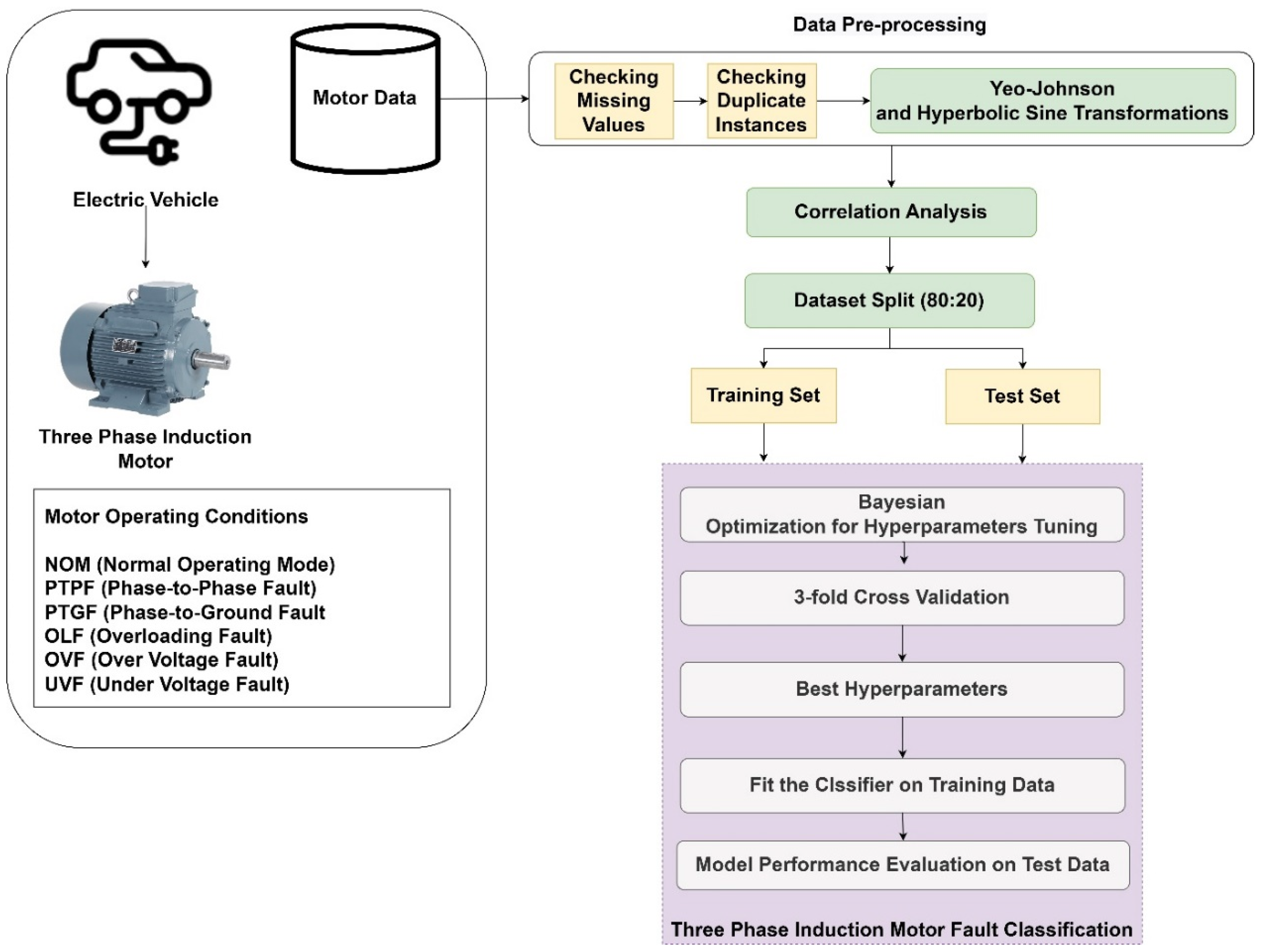
Figure 1 illustrates the workflow of the proposed fault classification model for a three-phase induction motor in an EV. The process started with motor data collection, which undergoes preprocessing steps, including checking for missing values and duplicate instances, followed by applying Yeo–Johnson and Hyperbolic Sine transformations to reduce skewness. After correlation analysis, the dataset was split into training and test sets in an 80:20 ratio.

The training set was then used for Bayesian optimization of hyperparameters, combined with three-fold cross-validation to determine the best parameters. The optimal classifier was then fitted to the training data. Finally, the model’s performance was evaluated using the test data to classify the motor operating conditions, which included NOM, PTPF, PTGF, OLF, OVF, and UVF.

2.1. Data

The dataset was used to detect the faults in AC electric drives used in EVs, particularly in VSDs that utilize three-phase IMs. It was designed to identify five specific faults using ML algorithms. The six operating conditions considered were NOM, PTPF, PTGF, OLF, OVF, and UVF.

The dataset [24] was generated using a Variable Frequency Drive (VFD) model simulated in MATLAB Simulink. Data were generated for different loading conditions relative to the full load torque of the motor [24], simulating real-world scenarios where motors operate under varying loads. A torque equation block was used to model different load levels relative to the motor’s rated torque. This block was used to simulate various load conditions, based on the equation (1.1852e⁻³) × u², where u represents the input voltage. The raw data from the simulations was captured as waveforms (time-series signals) and later transformed into a structured data matrix. The characteristics of the dataset are shown in

Table 1. Dataset characteristics.

Features	Count	Mean	Std	Min	25%	50%	75%	Max
Tn (rated torque) Nm	40,040	1.13875	0.37178	0.8	0.91875	1.0375	1.18125	2.5
k (constant of proportionality)	40,040	0.001349	0.000441	0.000948	0.001085	0.00123	0.0014	0.002964
Time (s)	40,040	0.25	0.144484	0	0.125	0.25	0.375	0.5
Ia (Amp)	40,040	17.89738	10.67385	0	11.47026	13.7461	23.35513	78.63935
Ib (Amp)	40,040	17.76482	10.47296	0	11.47008	13.78399	22.57296	79.11399
Ic (Amp)	40,037	18.46777	10.50953	0	11.74109	14.27437	24.03763	78.73894
Vab (V)	40,040	432.8393	123.434	0	389.6933	474.5666	474.9843	649.5165
Torque (N.m)	40,040	23.53362	59.28494	−404.838	19.15	26.66877	36.35022	625.1659
Speed (rad/s)	40,040	123.5214	49.80135	−112.258	132.8439	142.9008	147.744	182.5994

. The dataset contains nine features: Tn (rated torque) Nm, which is the rated torque in Newton meters (Nm); k (constant of proportionality), a constant used in the motor’s operational calculations; Ttme (sec), representing time in seconds; I_a (Amp), I_b (Amp), and I_c (Amp), which are phase currents in amperes; V_ab (V), the voltage between phases A and B, measured in volts; torque (Nm), the actual torque produced by the motor, measured in Nm; and speed (rad/s), the rotor speed, measured in radians per second. These features represent key aspects of the motor’s performance and are used to detect and classify various fault conditions. Negative torque (minimum value) represents braking or deceleration phases, during which the motor generates a reverse force to slow down or control the vehicle’s speed. Negative speed values indicate a reversal in the motor’s rotational direction.

The phase-to-phase and phase-to-ground faults were indicative of abnormal current paths, which physically result in overheating, increased electromagnetic forces, and potentially damaging vibration frequencies. The model’s input features, such as phase currents (I_a, I_b, I_c) and voltage (V_ab), were directly influenced by these conditions.

Overloading and over/under-voltage fault conditions directly impacted torque and speed characteristics, affecting the rated torque and speed variables in the dataset. An overloaded motor, for example, experiences excessive torque demand, which can lead to temperature rise and accelerated wear on mechanical components.

2.2. Data Preprocessing

The first step in model development was to identify any missing values in the dataset. In this dataset, only the feature I_c (Amp) has three missing values. Missing values can disrupt the analysis and ML model training process. If not handled, they could lead to incorrect model behavior or reduced performance [25]. Therefore, it was decided to remove the instances with missing values.

Next, the dataset was checked for duplicate rows, and a total of 1003 duplicates were found. Duplicates can distort the results of ML models by giving certain instances undue weight [26]. This can cause the model to overfit or misinterpret patterns, leading to inaccurate predictions. All identified duplicate rows were removed from the dataset, ensuring that it contained only unique instances and provided a more reliable and unbiased input for the ML model.

After preprocessing, the dataset contained 39,034 instances (rows) with no missing or duplicate values. The pie chart in Figure 2 presents the distribution of different fault conditions observed in the EV drive motor dataset. The faults included were NOM, PTPF, PTGF, OLF, OVF, and UVF.

In the dataset, the NOM condition, representing the motor running without any faults, constituted 33.3% of the total instances. Phase-to-phase fault (PTPF) and phase-to-ground fault (PTGF) were equally prevalent, each representing 18% of the dataset. The under-voltage fault (UVF) accounted for 7.69% of the total instances, followed by the over-voltage fault (OVF) at 10.3%, and finally, the overloading fault (OLF), which was 12.8% of the total dataset.

2.3. Data Transformation

The transformation process is crucial because many ML algorithms assume that the data is normally distributed. High skewness or kurtosis can lead to poor model performance, as it might distort relationships between features [27]. By reducing skewness and normalizing kurtosis, the data becomes more suitable for training ML models, improving the model’s ability to generalize well to unseen data.

In this data transformation process, two techniques were applied to address the skewness and kurtosis of several features in the data. All the features except the torque (N.m) feature were transformed using the Yeo–Johnson transformation, which is a power transformation technique that can handle both positive and negative values while aiming to make the data more normally distributed [28]. The Yeo–Johnson transformation is defined in Equation (1).

$$\mathsf{\psi }\left(\mathrm{y},\mathsf{\lambda }\right)=\left\{\begin{array}{cc}{\displaystyle \frac{{\left(\mathrm{y}+1\right)}^{\mathsf{\lambda }}-1}{\mathsf{\lambda }}}& \mathrm{y}\ge 0\mathrm{and}\mathsf{\lambda }\ne 0\\ \log (\mathrm{y}+1)& \mathrm{y}\ge 0\mathrm{and}\mathsf{\lambda }=0\\ {\displaystyle \frac{{\left(-\mathrm{y}+1\right)}^{\left(2-\mathsf{\lambda }\right)}-1}{2-\mathsf{\lambda }}}& \mathrm{y}<0\mathrm{and}\mathsf{\lambda }\ne 2\\ -\log (-\mathrm{y}+1)& \mathrm{y}<0\mathrm{and}\mathsf{\lambda }=2\end{array}\right.$$

(1)

where $\mathsf{\psi }$ is concave in ‘y’ for power parameter λ < 1 and convex for power parameter λ > 1.

Additionally, the Hyperbolic Sine (arcsinh) transformation was specifically applied to the torque (N.m) feature to further manage its skewness. The Hyperbolic Sine transformation for x is the original data value is defined in Equation (2) [29].

$$\mathrm{arcsinh}\left(x\right)=\ln (x+\sqrt{x^2+1})$$

(2)

Table 2. Comparison of skewness and kurtosis before and after applying Yeo–Johnson and Hyperbolic Sine transformations.

Feature	Before Transformation		After Transformation
	Skewness	Kurtosis	Skewness	Kurtosis
Tn (rated torque) N.m	2.171486	4.367023	0.199784	−0.532311
k (constant of proportionality)	2.167044	4.350688	0.308630	−0.522271
Time (s)	0.000002	−1.199999	−0.034996	−1.197256
Ia (Amp)	1.634488	4.624116	0.170565	1.725077
Ib (Amp)	1.482467	3.679726	0.153740	1.497030
Ic (Amp)	1.431171	3.582817	0.167173	1.597659
Vab (V)	−1.831005	4.462625	−0.916627	1.771581
Torque (N.m)	0.793944	26.522355	−2.235186	3.748812
Speed (rad/s)	−2.278316	3.961198	−1.935292	2.188660

shows the changes in skewness and kurtosis values for each feature after applying transformations, indicating improved data normality, which is crucial for better performance of ML models. The skewness of most features was significantly reduced after the transformations. The skewness of Tn (rated torque) dropped from 2.17 to 0.20, and for I_a (Amp), it decreased from 1.63 to 0.17. This indicates a more symmetric distribution after transformation, which is beneficial for many ML algorithms. The kurtosis values also show considerable improvement for most features. The kurtosis of k (constant of proportionality) decreased from 4.35 to −0.52, indicating that the transformed data is closer to a normal distribution. The reduction in kurtosis for torque (N.m) (from 26.52 to 3.75) reflects better distribution characteristics, though it still has some peakedness.

Figure 3 and Figure 4 present box plots comparing the distribution of various features before and after transformation. In Figure 3, the box plots depict the features in their original form, showcasing significant skewness and the presence of outliers, especially in features such as rated torque (Nm), phase currents (I_a, I_b, I_c), and actual torque (Nm).

In Figure 4, after applying transformations (Yeo–Johnson and Hyperbolic Sine), the box plots demonstrate a more normalized distribution with reduced skewness and fewer outliers. The transformations effectively compressed extreme values and made the data distributions more symmetric, improving the suitability of the features for ML models. The key features that show visible improvements after transformation include rated torque, phase currents, voltage (V_ab), and motor speed (rad/s). These transformations help in ensuring better performance and stability of the classification model.

2.4. Correlation Analysis

The correlation heatmap presented in Figure 5 shows the relationships between key features in the EV drive motor faults dataset. The most notable correlation is between T_n (rated torque) N.m and k (constant of proportionality), with a near-perfect positive correlation (0.999). Additionally, moderate positive correlations are observed between torque (N.m) and speed (rad/s) (0.502), as well as between phase currents (I_a, I_b, I_c), indicating a relationship between electrical and mechanical performance parameters.

Interestingly, there are negative correlations between speed (rad/s) and the phase currents, particularly with I_a (Amp) (−0.443) and I_b (Amp) (−0.489). This suggests an inverse relationship, where increased speed is associated with reduced current. The heatmap also shows that the correlation between features and the category (fault type) is relatively weak, suggesting that fault classification depends on a combination of features rather than a strong linear relationship with any single feature.

2.5. Machine Learning Algorithms

ML algorithms play a vital role in automating the detection and classification of faults in EV drive motors. By training on labeled data, these algorithms are designed to recognize patterns and relationships between motor features and fault conditions, enabling them to predict faults with high accuracy in real-world scenarios. The following subsections outline the four key ML algorithms used in this study: CatBoost, RF classifier, AdaBoost, and QDA.

2.5.1. CatBoost

CatBoost [30] was selected in the proposed method due to its ability to efficiently handle categorical data and mitigate overfitting, both crucial for accurate fault classification in electric vehicle drive motors. Its ordered boosting technique ensures robust model generalization, enhancing performance by preventing the use of future information during training.

Mathematically, the target assessment of the ith categorical data of the kth element of motor fault identification dataset D can be expressed as follows:

$${\widehat{x}}_k^i={\displaystyle \frac{\sum _{x_j\in D_k}1\left(x_k^i=x_k^j\right)y_j^c+a.p^c}{\sum _{x_j\in D_k}1\left(x_k^i=x_k^j\right)+a}};\mathrm{w}\mathrm{h}\mathrm{e}\mathrm{r}\mathrm{e}{D}_k=\left\{x_j:\sigma \left(j\right)<\sigma \left(i\right)\right\}$$

(3)

where $y_j^c$ represents the target label for each class ‘c’. The indicator function $1\left(x_k^i=x_k^j\right)$ outputs a value of 1 when the i-th component of input vector $x_j$ is equal to the ith component of input vector $x_k$; otherwise, it returns 0. For cases where a > 0, the indicator function $1(x_k^i=x_k^j)$ will return 1 when the two components are identical. The prior $p^c$ refers to class c, indicating that the prior is computed for each class to ensure the stability of the estimates in the presence of sparse data or small classes. The parameter ‘a’ is used as a smoothing factor to prevent underflow and help with cases where certain classes have very few data points. The permutation σ is applied to ensure the data is processed in a random order, which is crucial for the robustness of CatBoost’s categorical feature handling.

In the context of fault classification in EV drive motors, CatBoost is well-suited because it can handle the complexity and high-dimensional nature of the dataset, which contains multiple motor features that may have nonlinear relationships. By leveraging its gradient boosting approach, CatBoost iteratively builds an ensemble of decision trees that correct errors from previous iterations. The result is a highly accurate model that can classify faults under various operating conditions with minimal tuning. In this study, CatBoost demonstrated the highest classification accuracy across all fault categories, making it the most effective algorithm for the EV dataset.

2.5.2. Random Forest Classifier

RF is an ensemble learning method [31] that builds multiple decision trees during the training phase and combines their outputs to make predictions. In the proposed fault classification method, Random Forest (RF) is used to capture complex interactions among motor parameters (such as torque, speed, and currents) for accurate fault detection in EV drive motors. RF’s ensemble approach, combining multiple decision trees, enhances robustness against overfitting and provides reliable classification even with noisy data, making it well-suited for this application without extensive preprocessing.

2.5.3. AdaBoost

AdaBoost, or Adaptive Boosting, is another ensemble learning method that aims to improve the accuracy of weak classifiers by combining them into a strong classifier. It works by focusing on misclassified instances from the previous iteration and adjusting the weights accordingly so that subsequent models give more importance to difficult-to-classify cases [32]. AdaBoost is particularly useful for improving the performance of simple models like decision trees.

In this study, AdaBoost was applied to the EV drive motor dataset to classify fault conditions. Its strength lies in its ability to boost the performance of weaker classifiers and handle moderate levels of data imbalance. However, it may be more prone to overfitting compared to other ensemble methods, particularly in scenarios with noisy data or when the dataset is highly imbalanced across fault categories.

2.5.4. Quadratic Discriminant Analysis

QDA is a classification method that operates under the assumption that the data within each class is normally distributed. It extends Linear Discriminant Analysis (LDA) by allowing for a quadratic decision boundary between classes, making it more flexible in handling datasets with nonlinear relationships [33]. QDA models the covariance structure of each class separately, allowing it to capture more complex patterns in the data compared to LDA.

For fault classification in EV drive motors, QDA provides a simple yet effective approach when the dataset exhibits Gaussian-like distribution patterns for each class. However, QDA’s performance can degrade when the assumption of normality does not hold or when the dataset has high dimensionality and limited instances per class.

3. Results and Analysis

A total of 39,034 instances and nine features were used for the fault classification model development. The features represent various motor parameters such as rated torque (Nm), k (constant of proportionality), phase currents (Ia, Ib, Ic), time, voltage (Vab), actual torque (Nm), and motor speed (rad/s). Each instance corresponds to a set of measurements collected from EV drive motors, either in normal operating conditions or under specific fault scenarios. All experiments in this study were conducted using Python 3 with the Scikit-Learn, CatBoost, and Skopt libraries for machine learning model development and Bayesian optimization. The analyses were performed on the Google Colab cloud platform, which provided access to both GPU and CPU resources. This setup efficiently handled the computational demands of hyperparameter tuning, model training, and validation.

To prepare the dataset for ML model development, it was necessary to convert the categorical target variable, category, into numerical values. The category feature contains labels representing six different operating conditions: NOM, PTPF, PTGF, OLF, OVF, and UVF.

Each of these categorical values was mapped to a corresponding numerical value to make it suitable for use in ML algorithms. Specifically, NOM is mapped to 1, PTPF is mapped to 2, PTGF is mapped to 3, OLF is mapped to 4, OVF is mapped to 5, and UVF is mapped to 6.

By replacing the categorical labels with numerical values, the ‘Category’ feature was transformed into a numerical format, which can be used by ML models. This numerical encoding is essential for classification algorithms, as they require numeric inputs to process and learn from the data. The process of mapping categorical data into numerical form ensures that the ML model can effectively interpret and use the target variable for predicting fault types in EV drive motors.

The 39,034 instances were divided into training and test sets with an 80:20 ratio, respectively. The features represent the input variables that the model will use to make predictions, while the target variable category is the feature the model is being trained to predict. A random state (e.g., 42) was used to ensure reproducibility. Setting a specific random seed ensures that every time the data is split, the same training and test sets are generated, allowing for consistent results.

The model identifies patterns and correlations between the features and the target variable in the training set, allowing it to generalize and make accurate predictions on unseen data. The test set is held aside to assess the model’s performance on previously unseen data, offering an indication of how effectively the model is expected to perform in real-world applications.

3.1. Bayesian Optimization with Cross-Validation

Bayesian optimization was applied to each machine learning algorithm to identify the best set of hyperparameters, maximizing model performance with minimal computational cost. Unlike grid or random search, Bayesian optimization uses a probabilistic model to efficiently explore the hyperparameter space, quickly converging to optimal values by focusing on the most promising areas [34]. This is particularly beneficial for complex models where the hyperparameter space is high-dimensional.

For each machine learning model, the hyperparameter ranges were carefully selected based on prior knowledge of the algorithms, initial experiments, and specific requirements for fault classification in electric vehicle (EV) drive motors. Initially, the range of values to be explored by BayesSearchCV is defined for each ML algorithm. BayesSearchCV is set up to perform three-fold cross-validation, where the data is split into three parts, and the model is trained on different combinations of these parts.

For the random forest classifier, n_estimators were set between 100 and 150. This range was selected to limit the number of decision trees in the ensemble, balancing computational time with model accuracy. The ‘max_depth’ was constrained between 5 and 7 to control tree complexity, helping to avoid overfitting while ensuring sufficient model expressiveness. The ‘min_samples_split’ was restricted to values of 2 or 3, aiming to create deeper trees only where necessary, which is suitable for capturing complex patterns. The ‘min_samples_leaf’ was limited to 1 or 2 to prevent trees from becoming too granular and sensitive to small data fluctuations. The ‘max_features’ was fixed to ‘sqrt’, a commonly used value in random forests, which optimized the number of features considered for each split and balanced bias and variance.

For the CatBoost classifier, the ‘iterations’ ranged from 100 to 150, controlling the number of boosting rounds. A higher number of iterations allows for more fine-grained learning but risks overfitting, especially with smaller datasets. The ‘depth’ was set between 5 and 7 to control the depth of each tree, balancing model complexity with generalization ability. The ‘learning_rate’ was ranged between 0.01 and 0.3 on a logarithmic scale. This enables gradual learning to minimize the risk of overshooting optimal values, which is especially critical in boosting algorithms like CatBoost. The ‘l2_leaf_reg’, i.e., L2 regularization term on weights, was set between 1 and 10, acting as a regularization parameter to reduce overfitting by penalizing high model complexity.

For quadratic discriminant analysis, the regularization parameter ranges were chosen from 0.0 to 1.0 on a uniform scale, controlling the amount of regularization. Regularization is crucial in QDA to handle issues with high-dimensional data and avoid overfitting. The ‘Tolerance for stopping criteria’ was set between 1 × 10⁻⁵ and 0.1 on a logarithmic scale. This tolerance level determines the convergence threshold, helping to ensure model stability and efficient convergence.

For the AdaBoost classifier, ‘n_estimators’, i.e., the number of boosting iterations, was set between 50 and 150, controlling the number of boosting iterations. A lower number of estimators helps reduce computational load, while a higher number allows the model to learn more complex patterns. The ‘learning_rate’ parameter ranged from 0.01 to 1.0 on a logarithmic scale, adjusting the weight of each learner in the ensemble. Lower learning rates enable slower, more stable convergence, which can be beneficial for AdaBoost’s iterative nature.

Each model was optimized with BayesSearchCV and set to perform three-fold cross-validation. Cross-validation helps ensure robust performance by evaluating model accuracy on different data splits. Additionally, the number of iterations (n_iter = 10) was chosen to balance computational efficiency with a thorough exploration of the parameter space. The best cross-validation scores achieved during the search are provided in

Table 3. Hyperparameters and performance evaluation of various machine learning algorithms for fault classification.

ML Algorithm	Best Hyperparameters	Best Cross-Validation Score	Accuracy	Precision	Recall	f1-Score
CatBoost	(‘depth’, 6), (‘iterations’, 146), (‘l2_leaf_reg’, 2), (‘learning_rate’, 0.04366013678619019)	0.94	0.941	0.942	0.941	0.941
Random Forest Classifier	(‘max_depth’, 7), (‘max_features’, ‘sqrt’), (‘min_samples_leaf’, 1), (‘min_samples_split’, 3), (‘n_estimators’, 143)	0.927	0.932	0.938	0.932	0.932
AdaBoost	(‘learning_rate’, 0.010168587136004645), (‘n_estimators’, 132)	0.868	0.875	0.890	0.875	0.876
Quadratic Discriminant Analysis	(‘reg_param’, 0.8123959883573634), (‘tol’, 4.87 × 10−5)	0.854	0.865	0.869	0.8653	0.8659

for each ML algorithm.

3.2. Performance Evaluation of Machine Learning Algorithms for Fault Classification

The accuracy of the classification model was evaluated through performance metrics derived from the confusion matrix. Accuracy, precision, recall, and F1 score can be defined as shown in Equations (4), (5), (6), and (7), respectively [35]. The performance metrics help determine how well the optimized model generalizes to new, unseen data, which is critical for real-world ML applications.

$$\mathrm{\%}\mathrm{A}\mathrm{c}\mathrm{c}\mathrm{u}\mathrm{r}\mathrm{a}\mathrm{c}\mathrm{y}={\displaystyle \frac{\mathrm{T}\mathrm{r}\mathrm{u}\mathrm{e}\mathrm{P}\mathrm{o}\mathrm{s}\mathrm{i}\mathrm{t}\mathrm{i}\mathrm{v}\mathrm{e}+\mathrm{T}\mathrm{r}\mathrm{u}\mathrm{e}\mathrm{N}\mathrm{e}\mathrm{g}\mathrm{a}\mathrm{t}\mathrm{i}\mathrm{v}\mathrm{e}}{\mathrm{T}\mathrm{r}\mathrm{u}\mathrm{e}\mathrm{P}\mathrm{o}\mathrm{s}\mathrm{i}\mathrm{t}\mathrm{i}\mathrm{v}\mathrm{e}+\mathrm{T}\mathrm{r}\mathrm{u}\mathrm{e}\mathrm{N}\mathrm{e}\mathrm{g}\mathrm{a}\mathrm{t}\mathrm{i}\mathrm{v}\mathrm{e}+\mathrm{F}\mathrm{a}\mathrm{l}\mathrm{s}\mathrm{e}\mathrm{P}\mathrm{o}\mathrm{s}\mathrm{i}\mathrm{t}\mathrm{i}\mathrm{v}\mathrm{e}+\mathrm{F}\mathrm{a}\mathrm{l}\mathrm{s}\mathrm{e}\mathrm{N}\mathrm{e}\mathrm{g}\mathrm{a}\mathrm{t}\mathrm{i}\mathrm{v}\mathrm{e}}}\times 100$$

(4)

$$\mathrm{P}\mathrm{r}\mathrm{e}\mathrm{c}\mathrm{i}\mathrm{s}\mathrm{i}\mathrm{o}\mathrm{n}(\mathrm{p})=={\displaystyle \frac{\mathrm{T}\mathrm{r}\mathrm{u}\mathrm{e}\mathrm{P}\mathrm{o}\mathrm{s}\mathrm{i}\mathrm{t}\mathrm{i}\mathrm{v}\mathrm{e}}{\mathrm{T}\mathrm{r}\mathrm{u}\mathrm{e}\mathrm{P}\mathrm{o}\mathrm{s}\mathrm{i}\mathrm{t}\mathrm{i}\mathrm{v}\mathrm{e}+\mathrm{F}\mathrm{a}\mathrm{l}\mathrm{s}\mathrm{e}\mathrm{P}\mathrm{o}\mathrm{s}\mathrm{i}\mathrm{t}\mathrm{i}\mathrm{v}\mathrm{e}}}$$

(5)

$$\mathrm{R}\mathrm{e}\mathrm{c}\mathrm{a}\mathrm{l}\mathrm{l}(\mathrm{r})={\displaystyle \frac{\mathrm{T}\mathrm{r}\mathrm{u}\mathrm{e}\mathrm{P}\mathrm{o}\mathrm{s}\mathrm{i}\mathrm{t}\mathrm{i}\mathrm{v}\mathrm{e}}{\mathrm{T}\mathrm{r}\mathrm{u}\mathrm{e}\mathrm{P}\mathrm{o}\mathrm{s}\mathrm{i}\mathrm{t}\mathrm{i}\mathrm{v}\mathrm{e}+\mathrm{F}\mathrm{a}\mathrm{l}\mathrm{s}\mathrm{e}\mathrm{N}\mathrm{e}\mathrm{g}\mathrm{a}\mathrm{t}\mathrm{i}\mathrm{v}\mathrm{e}}}\times 100$$

(6)

$$\mathrm{f}1\mathrm{S}\mathrm{c}\mathrm{o}\mathrm{r}\mathrm{e}={\displaystyle \frac{(2\times \mathrm{p}\times \mathrm{r})}{(\mathrm{p}+\mathrm{r})}}$$

(7)

Table 3 presents the best hyperparameters identified through optimization, along with the cross-validation score, accuracy, precision, recall, and F1-score for each ML algorithm used in the study. CatBoost ML algorithm-based classification model demonstrated the highest performance, with a cross-validation score of 0.94, an accuracy of 0.941, and a precision, recall, and F1-score, all at 0.941. RF also performed well, with a best cross-validation score of 0.927 and accuracy of 0.932, while maintaining balanced precision, recall, and F1-score values. AdaBoost and QDA achieved lower scores, with AdaBoost having an accuracy of 0.875 and QDA showing an accuracy of 0.865, making CatBoost the most suitable algorithm for this classification task.

Table 4. Category-wise performance evaluation of various machine learning algorithms for fault classification.

ML Algorithm	Class	Precision	Recall	f1-Score
CatBoost	Class 0	0.9	0.94	0.92
	Class 1	0.96	0.88	0.92
	Class 2	0.92	0.92	0.92
	Class 3	1	1	1
	Class 4	0.99	0.99	0.99
	Class 5	1	0.98	0.99
Random Forest Classifier	Class 0	0.86	0.97	0.91
	Class 1	0.99	0.82	0.90
	Class 2	0.94	0.88	0.91
	Class 3	1	1	1
	Class 4	1	0.97	0.99
	Class 5	1	0.97	0.99
AdaBoost	Class 0	0.88	0.92	0.9
	Class 1	0.69	0.89	0.78
	Class 2	0.97	0.76	0.85
	Class 3	1	1	1
	Class 4	1	0.91	0.95
	Class 5	0.91	0.65	0.76
Quadratic Discriminant Analysis	Class 0	0.84	0.91	0.87
	Class 1	0.88	0.82	0.85
	Class 2	0.78	0.85	0.82
	Class 3	0.88	0.77	0.82
	Class 4	0.99	0.92	0.95
	Class 5	1	0.91	0.96

shows the performance of four ML algorithms (CatBoost, RF classifier, AdaBoost, and QDA) in classifying six different classes of faults. As per the confusion matrix and Table 3, NOM represents Class 0, PTPF represents Class 1, PTGF represents Class 2, OLF represents Class 3, OVF represents Class 4, and UVF represents Class 5. CatBoost consistently performs well across all classes, with near-perfect precision, recall, and F1-scores, particularly excelling in Class 3, Class 4, and Class 5 with scores of 1 or close to 1.

Similarly, the RF classifier demonstrated strong performance, with Class 3 and Class 4 receiving perfect F1-scores of 1. AdaBoost, while effective in some classes, struggled with lower performance in Class 1 and Class 5, showing a notable decrease in recall and F1-score. QDA showed moderate performance, with relatively lower F1-scores in Class 3 and Class 2 but remained strong in Class 4 and Class 5.

The CatBoost and RF classifier showed the most balanced performance across all classes, while AdaBoost and QDA exhibited greater variability in performance depending on the class.

Figure 6 shows the confusion matrices of the following ML classification models: (a) CatBoost, (b) RF classifier, (c) AdaBoost, and (d) QDA. The confusion matrix for each model reveals the classification performance across all classes. The confusion matrix breaks down predictions into true positives, false positives, true negatives, and false negatives for each class.

CatBoost classifier demonstrated the best overall performance, with high accuracy, precision, recall, and F1-scores across all classes. Misclassifications were minimal, making it the most reliable model for fault classification.

RF classifier also performed well, particularly in Classes 3, 4, and 5, but showed slightly more misclassifications in Classes 1 and 2 compared to CatBoost.

AdaBoost classifier showed acceptable performance in some classes but struggles significantly with Class 5, leading to lower overall effectiveness.

QDA had moderate performance but was less effective than the ensemble methods, particularly in Class 3, where it misclassified a substantial number of instances.

The superior performance of CatBoost suggests that it is highly effective at handling the complexities of the dataset, possibly due to its ability to handle categorical features and mitigate overfitting. For accurate and reliable fault detection in EV drive motors, CatBoost is the recommended classifier based on its exemplary performance in the confusion matrices.

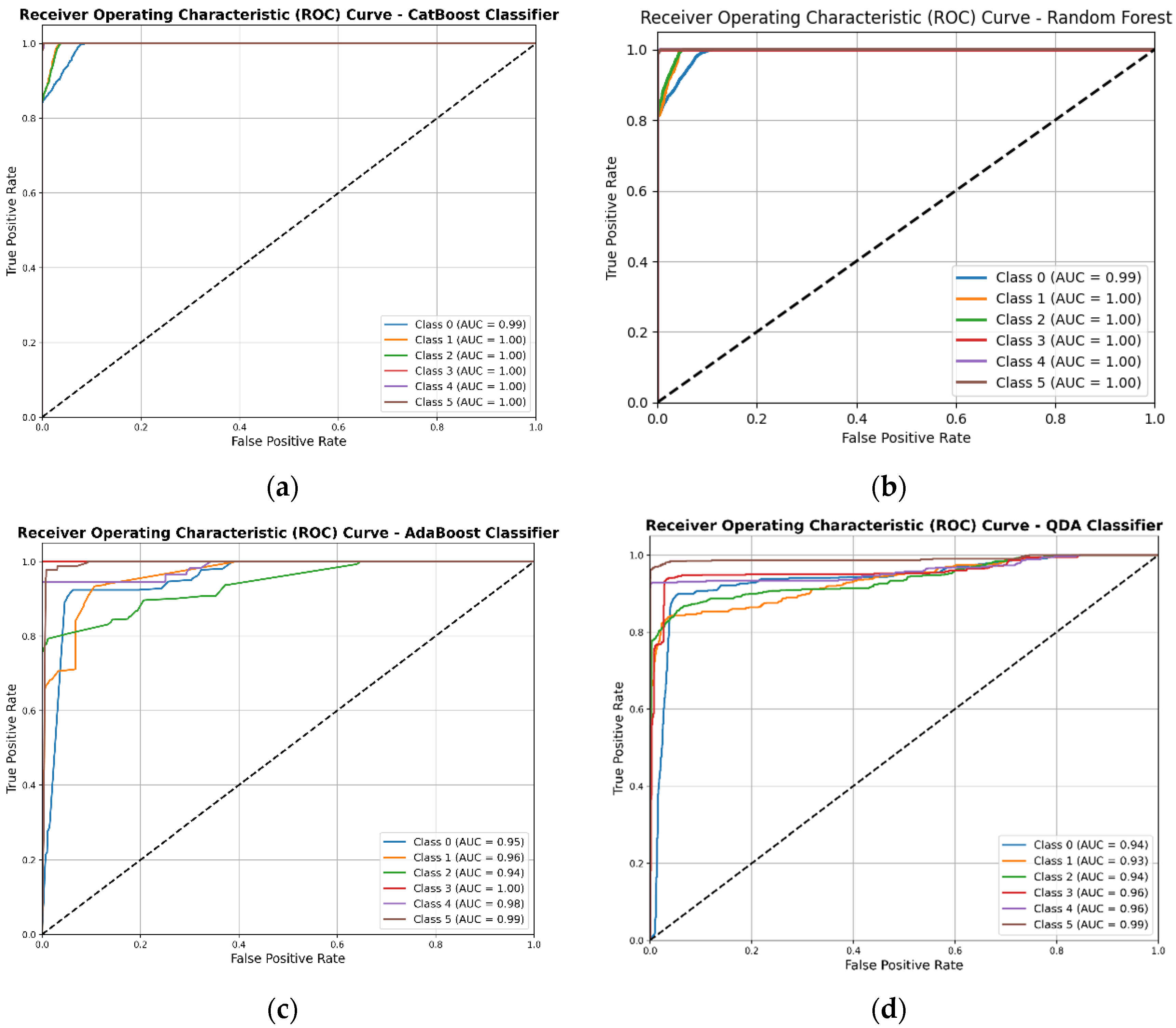
Figure 7 shows the receiver operating characteristic (ROC) curves for the classification of six fault classes in electric vehicle (EV) drive motors using four machine learning models: (a) CatBoost classifier, (b) RF classifier, (c) AdaBoost classifier, and (d) QDA. Each curve in the plots corresponds to one of the six classes: Class 0 (normal operating mode), Class 1 (phase-to-phase fault), Class 2 (phase-to-ground fault), Class 3 (overloading fault), Class 4 (over-voltage fault), and Class 5 (under-voltage fault).

Each plot displays the false positive rate (FPR) on the x-axis and the true positive rate (TPR) on the y-axis, representing the models’ capability to distinguish between fault classes. The diagonal dashed line indicates a random classifier with an area under the curve (AUC) of 0.5. The AUC values for each class are listed in the legends, providing a quantitative measure of each model’s performance. CatBoost showed nearly perfect classification performance, with AUC values close to 1.0 for all classes, making it highly effective for fault detection in this dataset. Similar to CatBoost, random forest also performed excellently, achieving AUC values close to 1.0 for each class. It demonstrated a strong ability to differentiate between fault types. While AdaBoost achieved high AUC values for most classes, it performed slightly less consistently across classes, with AUCs around 0.95 to 1.0, indicating minor variability in class differentiation. QDA provided moderate classification performance, with AUC values around 0.93 to 0.99. Although it performed well, it showed some limitations in comparison to ensemble models like CatBoost and Random Forest.

CatBoost, as a gradient boosting algorithm, generally had a higher computational overhead during training compared to simpler models. However, once trained, CatBoost’s inference time was relatively fast due to its use of optimized gradient boosting algorithms and efficient handling of categorical data. This characteristic makes it suitable for applications where frequent retraining is not required, and a well-trained model can be deployed for real-time predictions.

4. Conclusions

This research demonstrates the effectiveness of ML algorithms for fault classification in EV drive motors, particularly focusing on VSDs that utilize three-phase IMs. By transforming the data to reduce skewness and using Bayesian optimization for hyperparameter tuning, the ML models were able to classify six different fault conditions with high accuracy. Among the algorithms tested, CatBoost proved to be the most effective, achieving a cross-validation score of 0.94 and an accuracy of 94.1%, outperforming RF, AdaBoost, and quadratic discriminant analysis. The confusion matrix analysis shows that CatBoost excelled in accurately classifying faults across all categories, with minimal misclassifications. These findings underscore the importance of selecting appropriate data transformation techniques and employing advanced optimization methods for hyperparameter tuning to improve fault detection accuracy. Future research can extend this work by exploring more advanced deep learning techniques or integrating sensor data to further improve fault detection and diagnosis in EV drive motors.