A Study of Flexible Job-Shop Scheduling with Dual Constraints

Abstract

The flexible production job shop was selected as the research object, with the goal of minimizing the maximum completion time. A novel production scheduling model was devised by taking into account the sequence of occurrence of two distinct perturbations, namely preventive maintenance and emergency order insertion, within the same production scheduling plan. This was solved by an improved three-body crossover operator genetic algorithm. Finally, the superiority and effectiveness of the new production scheduling were demonstrated through an illustrative analysis.

1. Introduction

As consumer demand for diversified products increases, traditional production workshops are being superseded by more flexible alternatives. This is due to the fact that the fixed production processes typical of traditional workshops are unable to meet the flexible and changing demands of the modern market. In the context of actual production, the equipment, personnel, and production resources of the workshops are subject to constant change. Consequently, the occurrence of dynamic disturbance events, such as unexpected equipment failures and urgent order insertions, will significantly impair the efficacy and viability of the initial production planning, or even render it entirely inoperable. The aforementioned complexity and instability render the task of production scheduling more challenging.

Dynamic scheduling represents a flexible production workshop management strategy that demonstrates an excellent capacity to withstand interference. It effectively incorporates uncertain variables, such as the current production status and pending production tasks, into the production scheduling plan, thereby enabling real-time adjustments to guarantee seamless and efficient production processes. This approach not only enhances the flexibility and adaptability of the production process, but also significantly improves the workshop’s ability to respond to emergencies [1]. The most common sources of disruption include mechanical failures, order insertions, order urgency, and order postponement, among others [2].

In light of these uncertain factors, Zhu et al. [3] put forth a distributed flexible job-shop scheduling problem that takes order cancellation into account and devised an enhanced memetic algorithm (RMA) to address it. Silva et al. [4] constructed a mixed-integer linear programming model with the objective of minimizing work delays in the production scheduling of new orders involving parallel machines. Adil, B.; Fatma, S.M.; and Alper, H. [5] proposed a stochastic construction method for the dynamic/flexible job-shop scheduling problem. Many real-life-based decision-making mechanisms are incorporated in the scheduling mechanism, as well as designed event-driven and cycle rescheduling mechanisms. The superiority of the algorithm is demonstrated through extensive computational experiments. Gao, K.; Yang, F.; and Zhou, M. C. [6] designed a discrete Jaya algorithm-based solution for the rescheduling of new jobs inserted into a flexible job shop. Jomaa, Wahiba, Eddaly, Mansour et al. [7] put forth two variable neighborhood search algorithms to address the job-shop scheduling problem with considerations of equipment maintenance. In their study, Abdollahzadeh-Sangroudi [8] developed a maintenance plan for a job-shop production system based on the concept of dynamic opportunism.

As previously stated, the majority of research conducted by scholars has concentrated on the dynamic scheduling problem in the context of a single disturbance event. However, the actual disturbances observed in the production process are often more complex than those described in the literature. For instance, in the course of their research on shop floor production scheduling and emergency order insertion, the majority of scholars have operated under the assumption that the production state of the equipment remains constant. This is contrary to the empirical evidence that the longer equipment is in use, the higher the probability of equipment failure. It is therefore necessary to consider both the constraints of equipment pre-maintenance and emergency order insertion in production scheduling. The objective of this paper is to present a new scheduling strategy for the dynamic scheduling of flexible job shops, which takes into account two disturbances: equipment pre-maintenance and emergency order insertion.

2. Problem Description

The Flexible Job-Shop Scheduling Problem (FJSP) can be briefly described as a problem of the following type: n workpieces need to be processed, there are m related pieces of equipment in the production shop, and there are x (x ≦ m) pieces of equipment available for processing each process for each workpiece. Meanwhile, the following basic assumptions are usually made when studying the flexible shop floor scheduling problem:

(1) Each machine can process only one workpiece at a time;

(2) Each machine cannot be interrupted during the machining process;

(3) There is no equipment failure;

(4) Each machine is initially idle by default;

(5) The workpiece order has been determined and the machining priority of each workpiece is the same;

(6) Each workpiece can only be machined by one machine in the optional equipment set;

(7) During the production of each workpiece, the next process cannot be performed until the previous process has been completed.

However, in the actual production process, assumptions (3) and (5) are too idealized and do not meet the actual production requirements, so this paper focuses on the production scheduling of a flexible job shop that takes into account the need for equipment maintenance and dynamic orders.

3. Model Construction

The subject of this paper is the scheduling problem of a flexible production plant, and the objective of the study is to minimize the maximum completion time of the workpiece, and the objective function and its associated constraints can be expressed as follows:

$$C_{\max }=Min(\underset{1\le i\le n}{\mathrm{Max}}{(\mathrm{C}}_i\left)\right)$$

(1)

$$Star{t}_{ij}\ge En{d}_{i(j-1)}$$

(2)

$$En{d}_{ij}=Star{t}_{ij}+T_{ijk}$$

(3)

$${\displaystyle \sum _{i=1}^M{\alpha }_{ijk}=1}$$

(4)

Equation (1) represents the objective function; Equation (2) represents the process constraint of the workpiece, i.e., the production of the next process of the same workpiece will only start after the completion of the previous process; Equation (3) represents that the workpiece cannot be interrupted during the production process; and Equation (4) represents that each process of each workpiece can only be produced on a single machine.

$C_{\max }$ denotes the maximum completion time after the production of all workpieces; $C_i$ denotes the completion time of a workpiece $i$; $Star{t}_{ij}$ denotes the start time of the jth process of workpiece i; $En{d}_{i(j-1)}$ denotes the end time of the (j − 1) process of workpiece i; $T_{ijk}$ denotes the processing time of the jth process of workpiece i on equipment k; M denotes the number of workpieces; ${\alpha }_{ijk}$ is a decision variable and is taken to be 1 when the jth process of a workpiece is being processed on equipment k, otherwise it is taken to be 0.

In this paper, the solution process for equipment pre-maintenance and emergency order insertion in flexible production job-shop scheduling can be described as follows: the model prior to the emergency order insertion point is a scheduling model based on equipment pre-maintenance, while the model subsequent to the order insertion point is a collaborative scheduling model that considers both equipment pre-maintenance and emergency orders.

3.1. Pre-Maintenance

The necessity for preventative maintenance of equipment is contingent upon the reliability of the equipment in question. In the event that the failure rate of the equipment in question follows the Weibull distribution [9], the failure rate function is as follows:

$$f(t)={\displaystyle \frac{\beta }{\eta }}{({\displaystyle \frac{t}{\eta }})}^{\beta -1}$$

(5)

In the formula, the shape parameter and scaling parameter are represented as $\beta ,\eta$, and these can be obtained through historical data. The theoretical working time of the equipment is represented by $t$. From this formula, it can be observed that when the shape parameter is greater than 1, it aligns with the wear-out period of equipment failure, as outlined in reference.

Moreover, as the maintenance of the equipment in question is not of the highest standard, improvement factors [10] and fault rate adjustment factors [11] are introduced:

$$g_i={\left(a{\displaystyle \frac{c_p}{c_r}}\right)}^{b{\sqrt{c}}^{(1+\omega )}}$$

(6)

In the formula, $g_i$ represents the preventive maintenance improvement factor of equipment. $c_p,c_r$ respectively represent the cost of maintenance and replacement of equipment. $a,b,c$ respectively represent the cost adjustment coefficient, time adjustment coefficient, and maintenance times. $\omega$ is the learning effect adjustment coefficient, which is generally estimated by experts. The expression of the actual service life is derived after the $k$-th workpiece is processed:

$$\left\{\begin{array}{cc}{t}_k=t_0(1-g_i\cdot m_{i1})+u_{i1}& ,k=1\\ t_k=t_k^{+}=t_0{\displaystyle \prod _{j=1}^k(1-g_i\cdot m_{ij})+}{\displaystyle \sum _{j=1}^k{u}_{ij}{\displaystyle \prod _{h=1}^{j-1}(}1-g_i\cdot m_{ih})}& ,k\ge 2,j\ge 2\end{array}\right.$$

(7)

In the formula, the variable in question, $m_{ij}$, is a judgment variable. When the equipment $i$ is maintained before processing the $j$-th workpiece, the value is 1; otherwise, it is 0. $u_{ij}$ is the time required for the equipment $i$ to process the $j$-th workpiece. The symbol h denotes the workpiece that has been processed by device i prior to the j-th workpiece being processed.

In order to adjust the actual failure rate in accordance with the increase in equipment maintenance frequency, it is necessary to introduce a failure rate increasing factor:

$$mi{s}_i={\displaystyle \frac{c+L\cdot f{(t_0)}^{-1}}{L\cdot f{(t_0)}^{-1}}}$$

(8)

$$f_{t_k}=mi{s}_k\cdot {\displaystyle \frac{\beta }{\eta }}{({\displaystyle \frac{t}{\eta }})}^{\beta -1}$$

(9)

$mi{s}_i$ is the failure rate increasing factor of the equipment $i$ and $L$ is a constant. $f(t_0)$ is the failure rate at the initial moment. Through this formula, we can know that when there is a maintenance behavior for the equipment, the magnitude of the failure rate increasing factor is related to the number of equipment maintenance times and the value of $L$.

Accordingly, the reliability of the equipment following the processing of the $k$-th workpiece can be expressed as follows:

$$\left\{\begin{array}{cc}R(t_k)=\exp [-{({\displaystyle \frac{t_0(1-g_i\cdot m_{i1})+u_{i1}}{\eta }})}^{\beta }]& ,k=1\\ R(t_k)=\exp \{mi{s}_i[-{({\displaystyle \frac{t_0{\displaystyle \prod _{j=1}^k(1-g_i\cdot m_{ij})+}{\displaystyle \sum _{j=1}^k{u}_{ij}{\displaystyle \prod _{h=1}^{j-1}(1-g_i\cdot m_{ih})}}}{\eta }})}^{\beta }\text{}}& ,k\ge 2\end{array}\right.$$

(10)

In the event that the reliability value of the equipment in question falls below the established threshold, it is imperative that the requisite preventive maintenance procedures be undertaken with the utmost urgency.

3.2. Order Insertion

3.2.1. Order Priority

Prior to undertaking an investigation into order insertion, it is essential to make the following assumptions:

(1) The production process is subject to a single instance of interference;

(2) The process involves the insertion of multiple orders.

A review of the literature reveals that the majority of scholars adhere to two primary research approaches when investigating order insertion. The first hypothesis is that order insertion interference occurs only once and that the priority of the inserted order is not considered after insertion. The second hypothesis is that order insertion occurs only once and that the priority of the inserted order is assumed to be higher than that of the initial order. The primary focus of this article is the examination of production rescheduling, with a particular emphasis on the prioritization of inserted orders.

The determination of order priority is primarily based on the TOPSIS method, a comprehensive weighting approach, the grey relational analysis method [12], the RBF neural network model method [13], and the correlation matrix method [14], among others. From reading several studies, it is clear that the weighted grey relational analysis method is an effective approach for determining order priorities. The objective of this article is to determine the priority of insertion orders by combining the entropy weighting method with the grey relational analysis method.

Entropy Weight Method

In the event that there are n orders that require urgent insertion into the production process and m evaluation indicators, an evaluation decision matrix, $\mathrm{X}={(x_{ij})}_{n\times m}$, can be obtained for each order. In order to facilitate comparison between the different dimensions and numerical sizes, it is necessary to carry out dimensionless processing of the data in order to obtain a standardized decision matrix Z. The processing formula is as follows:

$$z_{ij}={\displaystyle \frac{x_{ij}-\min (x_{1j},x_{2j},\dots x_{nj})}{\max (x_{1j},x_{2j},\dots x_{nj})-\min (x_{1j},x_{2j},\dots ,x_{nj})}}$$

(11)

Then, the probability matrix P is calculated, and the calculation formula for each element $p_{ij}$ in P is as follows:

$$p_{ij}={\displaystyle \frac{z_{ij}}{\sqrt{{\displaystyle {\sum }_{i=1}^n{z}_{ij}}}}}$$

(12)

Then, the information entropy can be calculated by Boltzmann’s formula, and the expression is as follows:

$$e_j=-{\displaystyle \frac{1}{\ln (n)}}{\displaystyle \sum _{i=1}^n{p}_{ij}\ln (}{p}_{ij}),(j=1,2,3\dots ,m)$$

(13)

The information redundancy degree is $d_j=1-e_j$, and the entropy weight of each evaluation index can be obtained by normalizing the information redundancy degree:

$${\omega }_j={\displaystyle \frac{d_j}{{\displaystyle {\sum }_{j=1}^m{d}_j}}}$$

(14)

The combination of the entropy weighting and the grey relational analysis method allows the priority order of each emergency order to be determined.

Grey Correlation Analysis Method

Grey correlation analysis comprises five principal stages: data dimensionless processing, determination of the reference sequence, determination of the weight, calculation of the grey correlation coefficient, and calculation of the grey weighted correlation degree.

In the context of grey relational analysis, if the initial evaluation matrix is designated as X, the dimensionless processing formula can be expressed as follows:

$$x_{ij}={\displaystyle \frac{x_{ij}^{\prime }}{\frac{1}{m}{\displaystyle {\sum }_{j=1}^m{x}_{ij}^{\prime }}}}$$

(15)

In the formula, $x_{ij}^{\prime }$ is the value of the j-th evaluation index for order i in matrix X, and $x_{ij}$ is the corresponding value after dimensionless processing.

To standardize the dimensionless matrix, the formula is as follows:

$$y_{ij}={\displaystyle \frac{x_{ij}}{\sqrt{{\displaystyle {\sum }_{i=1}^n{x_{ij}}^2}}}}$$

(16)

By taking this step, we can obtain the normalized matrix $B_{ij}={(y_{ij})}_{n\times m}$. According to the formula $c_{ij}={\omega }_j\times y_{ij}$, we obtain the weighted normalized matrix $C={(c_{ij})}_{n\times m}$. Now, we need to normalize matrix C to obtain the final matrix $C^1={(c_{ij}^1)}_{n\times m}$. The formulas are as follows:

Normalization formula for cost indicators:

$$c_{ij}^1={\displaystyle \frac{\underset{i}{\max } c_{ij}-c_{ij}}{\underset{i}{\max } c_{ij}-\underset{i}{\min } c_{ij}}}$$

(17)

Normalization formula for benefit-oriented metrics:

$$c_{ij}^1={\displaystyle \frac{c_{ij}-\underset{i}{\min } c_{ij}}{\underset{i}{\max } c_{ij}-\underset{i}{\min } c_{ij}}}$$

(18)

In the formulas, the symbols $\underset{i}{\max } c_{ij}$ and $\underset{i}{\min } c_{ij}$ represent the maximum and minimum values of the index j, respectively.

Since the data after normalization all belong to the range of 0–1, the reference sequence $A0=(1,\dots ,1)$ is chosen as the sequence. The calculation formula for the grey relational coefficient is as follows:

$${\zeta }_{ij}={\displaystyle \frac{\underset{i}{\min } \underset{j}{\min }\left|A{0}_j-c_{ij}^1\right|+\rho \times \underset{i}{\max } \underset{j}{\max }\left|A{0}_j-c_{ij}^1\right|}{\left|A{0}_j-c_{ij}^1\right|+\rho \times \underset{i}{\max } \underset{j}{\max }\left|A{0}_j-c_{ij}^1\right|}}$$

(19)

In the formula, $\left|A{0}_j-c_{ij}^1\right|$ represents the absolute value of the difference between each data point and the corresponding data point in the reference sequence. $\rho$ represents the resolution coefficient, whose value range is [0, 1] and is typically taken as 0.5.

The grey weighted correlation degree $r_i$, which represents the priority of each order, can be determined on the basis of the calculated weights and grey correlation coefficients:

$$r_i={\displaystyle \frac{1}{m}}{\displaystyle \sum _{j=1}^m{\zeta }_{ij}}$$

(20)

3.2.2. Insertion Strategy

In the study of the problem of inserting orders, three main considerations emerge: the time of order insertion, the determination of the priority of the inserted order, and the selection of the scheduling plan after insertion. The preceding text has already delineated the methodology for determining the priority of orders. This section will focus on the subsequent rescheduling process following the insertion of orders.

Prior to rescheduling, it is essential to evaluate the status of each workpiece’s processing stages as originally scheduled.

1. In the event that the completion time of the operation precedes the commencement of the disturbance, the operation is categorized as a completed operation and $Fa$ is represented by the symbol;

2. If the start time of the operation is earlier than the start time of the disturbance but the completion time is later than that time, the operation is placed into the processing operation set, denoted as $Ma$;

3. If the start time of the operation is later than the start time of the disturbance, the operation is placed into the to-be-processed operation set, denoted as $Wa$.

As the set $Fa$ has been completed prior to the insertion of the order, the process steps within the set remain in their original positions. Furthermore, it is assumed that the equipment cannot be interrupted during the processing stage, and thus the positions of the process steps in the set $Ma$ remain unchanged. At this juncture, the process steps within the set $Wa$ should be merged with the inserted order for the purpose of rescheduling. The rescheduling process entails the designation of a priority processing channel, contingent upon the priority level of the inserted order. This ensures the selection of production equipment with superior comprehensive capabilities or higher capability levels. The expression is as follows:

$$M_k(O_{ij})=rand(M_{ij}⌈(1-r_i)l_{ij}+1⌉)$$

(21)

In the formula, $M_k(O_{ij})$ represents the set of available equipment for the j-th process of an order i; $M_{ij}$ represents the set of available equipment for the j-th process of an order i, sorted in ascending order of processing time; ⌈ ⌉ represents rounding up; $r_i\in (0,1]$ is the priority coefficient of an order; $l_{ij}$ is the number of available equipment for the j-th process of an order i.

The general order insertion methods are order cancellation and insertion, deferred order insertion, and rearrangement of order insertion. In light of the fact that the inserted orders are of varying priority, this article employs the method of matching and deferred order insertion for rescheduling, thereby ensuring that the orders with the highest priority are given precedence in the context of production scheduling.

3.3. Algorithm Design

The principal stages of the conventional genetic algorithm encompass population initialization, selection, crossover, mutation, and additional operational modules. In the process of enhancing the algorithm, the research is primarily concentrated on four key areas: the generation of the initial population, the selection operator, the chromosome crossover, and the mutation. The objective of this article is to present an improvement to the chromosome crossover operator (Figure 1).

3.3.1. Crossover Operator

The determination of crossover probability $PC$ and mutation probability $PM$ represents a significant factor influencing the efficacy of genetic algorithms. In theory, an excessive or insufficient value of $PC$ will have a detrimental impact on the population. In order to minimize such effects, the concept of adaptive crossover is introduced, and the expression for adaptive probability is as follows:

$$P_c=\left\{\begin{array}{cc}{P}_{c1}\ast {\displaystyle \frac{f_{\max }-f^{\prime }}{f_{\max }-f_{ave}}},& f^{\prime }>f_{ave}\\ P_{c1},& f^{\prime }<f_{ave}\end{array}\right.$$

(22)

In the formula, $P_{c1}$ represents the given crossover probability, $f_{\max }$ represents the maximum fitness value of all chromosomes in the current population, $f^{\prime }$ represents the fitness value of the chromosome being judged for crossover operation, and $f_{ave}$ represents the average fitness value of the population.

The aforementioned expression has the potential to enhance the singularity issue of chromosomes in the population at the later stage of the iteration process. However, it is observed to exert an adverse effect on the initial stage of the iteration process. It is therefore evident that further improvement is required. The enhanced crossover probability is delineated as follows:

$$P_c=\left\{\begin{array}{cc}{P}_{c1}-{\displaystyle \frac{(P_{c1}-P_{c2})(f^{’}-f_{ave})}{f_{\max }-f_{ave}}},& f^{\prime }\ge f_{ave}\\ P_{c1},& f^{\prime }<f_{ave}\end{array}\right.$$

(23)

In the formula, $P_{c2}$ represents a custom crossover probability. Since the chromosome consists of two parts, namely equipment and process, there are two crossover methods: equipment chromosome crossover and process chromosome crossover. Therefore, a parameter $Pw(0<Pw<1)$ is specified to determine which crossover method the chromosome should choose.

Device Chromosome Crossover

This article adopts the uniform crossover method for equipment chromosome crossover. The specific operation is shown in Figure 2.

Process Chromosome Crossover

In the course of conducting crossover operations for process chromosomes, the text makes use of the Precedence-Preserving Order-Based Crossover (POX) method, as detailed in reference [15], with the particular operation depicted in Figure 3.

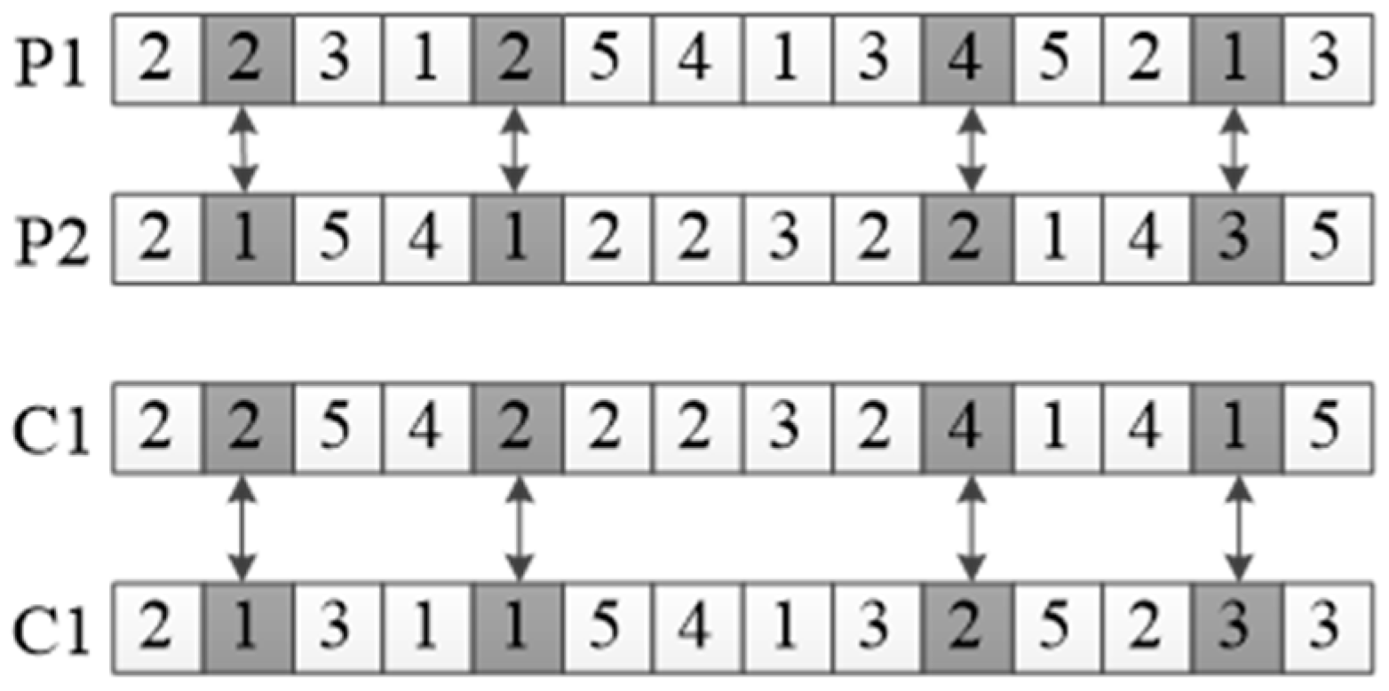
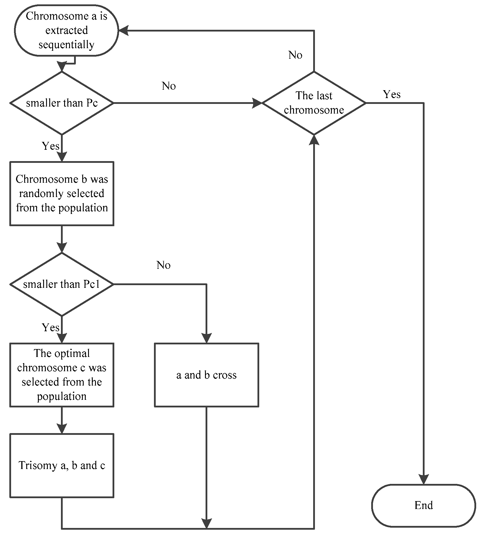
In order to ensure that the offspring chromosome obtained following crossover incorporates the superior genes of the parent generation, accelerates the convergence of the population, and rapidly identifies the optimal solution, this article employs a tri-parent crossover operator within the algorithm, as illustrated in Figure 4. In the aforementioned figure, Pc1 represents the probability of a crossover event, while Pc3 denotes the probability of a tri-parent crossover event. The particular operation of the three-body crossover is illustrated in Figure 5. The principal stages of tri-parent crossover are as follows:

Step 1: Select the individual c with the best fitness value in the population;

Step 2: The crossover method of the chromosome must be determined. Individual c must be crossed with two other individuals, a and b, respectively. The remaining parts of a and b must then be crossover to obtain offspring d1 and d2.

3.3.2. Mutation Operator

Adaptive mutation probability is introduced, and the expression is as follows:

$$P_m=\left\{\begin{array}{cc}{P}_{m1}-{\displaystyle \frac{(P_{m1}-P_{m2})(f-f_{ave})}{f_{\max }-f_{ave}}},& f\ge f_{ave}\\ P_{m1},& f<f_{ave}\end{array}\right.$$

(24)

In the formula, $P_{m1}$ represents the fixed mutation probability and $P_{m2}$ represents the custom mutation probability. Similar to crossover operator, mutation in the chromosome has two modes: device chromosome mutation and operation sequence chromosome mutation.

The mutation of chromosomes plays an essential role in maintaining the diversity of the population. During the process of mutation, the sequence of operations that comprise the chromosome’s operational layer remains unaltered; however, the device layer is subject to mutation.

In order to select the device chromosome, a random selection of m positions should be made on the chromosome, and the equipment at those positions should be set as the optimal equipment among the currently selectable equipment.

3.3.3. Determination of Local Population Convergence

During the course of its iterations, the genetic algorithm is susceptible to falling into a local optimum. This article applies the method of particle swarm population state determination, as outlined in reference [16], to the genetic algorithm. The introduction of fitness variance allows for the real-time monitoring of population deviation, thereby facilitating the timely adjustment of the current population evolution mode. The expression of the population fitness variance is as follows:

$${\delta }^2={\displaystyle \frac{1}{N}}{\displaystyle \sum _{i=1}^N{(f_i-f_{ave})}^2}$$

(25)

In the formula, N represents the number of chromosomes in the population, $f_i$ represents the fitness value of chromosome i, and $f_{ave}$ represents the average fitness value of all chromosomes in the population. During the iteration process of the algorithm, when ${\delta }^2\approx 0$, the optimal value is found or the algorithm falls into local convergence, it is likely that the diversity of chromosomes in the population is relatively rich when ${\delta }^2\gg 0$. If ${\delta }^2\to 0$ or remains unchanged within a certain fixed range, it indicates that the diversity of chromosomes in the population has significantly decreased, and the population tends to converge prematurely towards a local optimal solution.

It is stipulated that when the number of iterations of the population is less than three-fourths of the total number of iterations and the value ${\delta }^2$ is less than or equal to 0.1, this indicates that the population has fallen into a local optimal solution. In order to avoid the local optimal solution, the following steps may be taken:

Step 1: Randomly generate a new population C1 of the same size as the original population.

Step 2: The fitness values of each chromosome in the new population should be compared and subsequently sorted in descending order. The upper third or quarter of the chromosomes from the initial population should be transferred to the new population C2.

Step 3: The chromosomes in the original population should be sorted in descending order of fitness values, and the top quarter of the chromosomes should be selected for addition to the new population.

Step 4: The newly formed population, designated C2, is then assigned to the original population, C, and the iterative operation of the algorithm is continued.

4. Case Analysis

In order to test and improve the performance of the algorithm, a simulation is conducted in Python software of version 3.9 on a computer with a 64-bit Windows 11 operating system. The computer is equipped with an AMD Ryzen 7 5700U CPU with Radeon Graphics, operating at 3.2 GHz, and has a base memory of 16 GB. The experiment is divided into two distinct sections. The initial phase of the study is designed to validate the efficacy of the preventive maintenance strategy proposed in this article by comparing it with right-shift preventive maintenance and periodic maintenance strategies through the use of case studies. The second part is a comprehensive study on dynamic scheduling that considers the integration of preventive maintenance and order insertion.

4.1. Verifying the Validity of Maintenance Policies

The comparison of preventive maintenance strategies is based on the data from a machining workshop in a hydraulic component manufacturing enterprise, as detailed in

Table 1. Information about each device.

	Device 1	Device 2	Device 3	Device 4	Device 5	Device 6
Initial age/Working time (sec.)	60	20	20	30	10	10
Initial total maintenance times	0	10	127	253	30	18
Reliability threshold	0.85	0.85	0.90	0.85	0.85	0.88
Time spent on a single maintenance	15	10	12	15	8	10
A single fault takes time to maintain	30	20	24	30	16	20
Replacement cost (CNY)	60,000	80,000	80,000	80,000	80,000	80,000
Single maintenance cost (CNY)	380	420	450	400	405	360
Scale parameter	151.1	158.9	158.2	152.9	169.5	153.5
Shape parameter	2.98	3.12	2.91	3.10	3.01	2.98

. In accordance with the literature [17], the cost adjustment coefficient a and the time adjustment coefficient b can be taken as 1 and 0.07, respectively [17]. Additionally, the learning adjustment coefficient $\omega =-0.355$ is also included.

In order to identify the optimal processing plan, the dynamic predictive maintenance strategy presented in this paper, in conjunction with the right-shift preventive maintenance and periodic maintenance strategies, was executed 10 times. As illustrated in the table, the maintenance times of the predictive maintenance strategy presented in this paper are five times, which represent the shortest maintenance times among the three maintenance strategies. Secondly, the right-shift strategy preventive maintenance, despite exhibiting maintenance times that are comparable to those of the predictive maintenance strategy presented in this paper, displays a considerably longer completion time. The periodic maintenance strategy demonstrated the poorest performance. In comparison, it can be seen that the predictive maintenance strategy presented in this paper is effective in practical application (

Table 2. Information about each device.

Maintenance Strategy	Completion Time	Maintenance Number	Maintenance Cost (CNY)
Immediate preventive maintenance	124	5	2010
Right-shift strategy preventive maintenance	132	6	2415
Periodic maintenance	154	8	3195

).

Figure 6, Figure 7 and Figure 8 illustrate three distinct strategy Gantt charts for preventive maintenance, wherein the numerals 1–10 within the Gantt rectangles signify the number of workpieces, and the letter P denotes equipment maintenance.

A comparative analysis of Gantt charts representing three distinct strategies indicates that the optimal shift maintenance and cycle maintenance strategies result in a greater number of idle time periods during the production process. The preventive maintenance strategy proposed in this paper allows for maintenance to be conducted before the machine age threshold is reached. By adopting forward shifting and right-shift maintenance, the maintenance plan can be arranged as much as possible in the idle time period before the age threshold, thereby verifying the effectiveness of the greedy insertion decoding method that takes preventive maintenance into account.

4.2. Integrated Scheduling Research

For the purposes of comparison, the processing workshop information provided in the literature [17] is still used here, and it is assumed that the workshop is a 6 × 6 flexible job-shop scheduling type. Subsequently, orders 7 to 10 will be incorporated into the production scheduling as insertion orders. The operations that have not been processed by the insertion time of the orders will be calculated together with the insertion orders for priority. The relevant information pertaining to the priority judgment indicators is presented in

Table 3. Priority determination indicator.

Order Number	Product Type	Resource Satisfaction	Customer Importance	Order Revenue	System Reliability	Yield	Date of Delivery	Production Cost	Technological Level
Order 1	0.25	0.65	0.43	0.54	0.67	0.71	0.5	0.43	0.45
Order 2	0.30	0.55	0.44	0.55	0.66	0.73	0.52	0.44	0.39
Order 3	0.27	0.66	0.50	0.58	0.65	0.67	0.48	0.51	0.47
Order 4	0.29	0.70	0.24	0.61	0.65	0.66	0.49	0.56	0.50
Order 5	0.31	0.68	0.38	0.51	0.64	0.68	0.55	0.40	0.38
Order 6	0.28	0.71	0.48	0.52	0.69	0.70	0.53	0.39	0.32
Order 7	0.51	0.74	0.74	0.64	0.75	0.62	0.58	0.44	0.53
Order 8	0.62	0.78	0.75	0.62	0.74	0.65	0.62	0.54	0.61
Order 9	0.37	0.62	0.69	0.69	0.71	0.68	0.59	0.66	0.58
Order 10	0.55	0.71	0.65	0.72	0.76	0.75	0.69	0.59	0.65

.

The information presented in the table allows the user to ascertain the priority order of all orders subsequent to the insertion time. If only the priority of the insertion order is considered, the order of insertion priorities is obtained as follows: 8, 10, 9, 3, 6, 5, 2, 4, 1, 7. The order of insertion priorities is obtained as 10, 7, 9, 8. The order insertion method in this paper and the method of complete rescheduling of all processes in order of priority after the order insertion time are run independently 10 times, with the objective of identifying the shortest completion time. The optimal results are then compared. When the order insertion time is 20, 30, and 50, the results presented in

Table 4. Order insertion strategy results comparison.

Order Insertion Strategy	Insertion Time = 20 s	Insertion Time = 30 s	Insertion Time = 50 s
Full rescheduling strategy for only urgent insertion orders after the insertion moment	130	131	137
Full rescheduling policy after the insertion moment	165	163	157

are obtained.

As illustrated in the above table, when the order insertion time is 20, 30, and 50, respectively, the results obtained by the order insertion strategy proposed in this paper (full rescheduling strategy for only urgent insertion orders after the insertion moment) are superior to those yielded by the complete rescheduling strategy based on the order insertion time. Figure 9 and Figure 10 illustrate the Gantt chart for the scenario where the order insertion time is 20.

5. Conclusions

This paper presents a production scheduling model based on the traditional flexible job-shop scheduling approach, with the objective of optimizing equipment completion time. The model considers the impact of preventive maintenance and order insertion on equipment availability. Concurrently, the conventional genetic algorithm is enhanced with the introduction of novel operators, namely adaptive crossover, variance function, and three-body crossover. Additionally, a novel approach to dynamic preventive maintenance is proposed, taking into account the inherent limitations in equipment maintenance and a priority processing channel strategy based on the insertion order priority. In terms of experimentation, the advantages of the preventive maintenance strategy proposed in this paper are first verified by comparing the differences between three maintenance strategies with examples. Secondly, the proposed strategy is compared with the target value obtained by the complete rescheduling strategy based on different order insertion times, taking into account the conditions of equipment maintenance and order insertion. This comparison demonstrates the effectiveness and superiority of the proposed strategy.

To align the research with the actual production situation, the single-objective research should be extended to multi-objective research in the subsequent research process. This could include setting the objective function as the shortest order completion time, the smallest equipment energy consumption, and the smallest delay time of inserting the order. This approach would make the research more practical.

Concurrently, the investigation revealed that as the quantity of workpieces and the number of machining devices increase, the solution speed of the model markedly declines. Subsequent to this, the potential for integrating distributed computing or combining machine-learning techniques with genetic algorithms for predictive maintenance may be contemplated, as this could further enhance the model’s adaptability and robustness.