Numerical Investigation of Complex Hydraulic Fracture Propagation in Shale Formation

Abstract

Due to the high flow resistance of shale oil and gas, creating artificial flow channels with high conductivity in shale formation was the main challenge for the development of shale oil and gas resources. To further understand the fracture propagation mechanism in shale formation, this paper proposed a global cohesive element method to simulate the hydraulic fracture propagation behavior in which natural fractures were distributed randomly, and the fracture geometry was quantitatively analyzed. From the simulation, it can be found that the horizontal stress difference was the determining factor affecting the generation of a complex fracture network. The simulation indicated that a low horizontal stress difference was beneficial for improving the stimulated volume. When the stress difference was below 5.0 MPa, numerous branch fractures were created which was the foundation of a complex fracture network. High injection rates with low-viscosity fracturing fluid were helpful for creating a complex fracture network, while high-viscosity fracturing fluid limited the fracture fluid flow into the deep formation.

1. Introduction

Due to the abundance of oil and gas resources in shale formations, shale oil and gas resources have become the most promising energy sources to support industrial production. Limited by the low permeability and porosity of shale formations, hydraulic fracturing has become the key technology for the effective development of shale oil and gas [1,2,3].

During the recent decades, many experiments and simulation results were conducted to understand the mechanism of complex fracture network formation [4]. The experiments and simulations indicated that horizontal stress difference was the main factor affecting the interaction between a natural fracture and a hydraulic fracture [5,6]. With experimental research, it was demonstrated that when HFs interact with NFs, different mechanical properties and approach angles may lead to different interaction results. The laboratory can only study a fracture geometry with limited factors [7,8,9]. In addition, it was difficult to observe the fracture network extension in these experiments because the scale of core samples was too small, which was far from the reservoir scale. Recently, many simulation models were established based on the FEM, DEM, and DDM. During the simulation, the fracture propagation trajectory was pre-determined, it was difficult to simulate the interaction between a hydraulic fracture with multiple natural fractures [10,11]. Based on previous research, it is indicated that three different styles were displayed when the hydraulic fracture interacted with a natural fracture, namely crossing, arrest, and offset. The fracture geometry in interaction with a natural fracture was comprehensively affected by the horizontal stress difference, approach angle, injection rate, and viscosity of fracturing fluid [12,13]. To overcome the barrier of horizontal stress differences on complex fracture networks, some experiments and simulations were conducted to investigate the cluster space, injection rate, and viscosity of fracturing fluid on fracture propagation [14,15,16]. The simulations showed that cluster space was the main factor affecting the fracture propagation, increasing the injection rate can release the “stress shadow” on fracture propagation under certain cluster spaces. It also showed that temporary plugging and diverting fracturing was an effective method to increase the number of branch fractures during multi-staged hydraulic fracturing [17,18].

To further investigate hydraulic fracture propagation in shale formations abundant in natural fractures, this paper proposed a global cohesive method to simulate and analyze the complex fracture network. Compared with previous research on fracture propagation behavior using CZM, the method proposed in this paper has the advantages as follows. In previous research, most studies focused on single fractures and the interaction of single fractures under the influence of geological and engineering factors, which only represent local correlations within the reservoir. At the same time, the path of fracture propagation should be strictly planned. The cohesive elements were inserted in the whole reservoir model randomly, the distribution of weak surfaces was generally more complicated. The randomly occurring and distributed weak surfaces in the model were closer to the real reservoir, which can more accurately simulate the extension of hydraulic fractures under multi-weak surfaces. During the simulations, the effects of mechanical rock properties, ground stress fields, and injection parameters on fracture network generation were analyzed. This provided a new method to optimize the hydraulic fracture processing parameters during the exploration and development of shale oil and gas.

2. Governing Equation

The physical processes of hydraulic fracturing can be divided into four processes: (1) fracture initiation; (2) Fracturing fluid flows in the fracture network, including tangential flow in the fracture and normal flow in the rock matrix; (3) extension of natural fractures; (4) Fracturing fluid causes deformation of rock around fractures.

2.1. Stress Equilibrium Equation

In the simulation, the principle of effective stress was used to describe the coupling between the stress field of the rock matrix and fluid pressure, as shown below [19]:

$${\sigma }_{total}=\sigma \prime +\alpha P_w\delta$$

(1)

where ${\sigma }_{total}$ is the total stress; $\sigma \prime$ is the tensor of the effective stress; $\alpha$ is the Biot coefficient; P_w is the pore pressure; and δ is the Kronecker constant.

During fracture propagation, the rock surface deformation caused by the fracturing fluid injection was described by the virtual work principle, which was defined as follows [20]:

$${\displaystyle \int (\overline{\sigma }-p_{w}I)}:\delta \epsilon dV={\displaystyle {\int }_{S}t\cdot }\delta vdS+{\displaystyle {\int }_{V}f\cdot }\delta vdV$$

(2)

where $\overline{\sigma }$′ and $\epsilon$′ are effective stress and virtual deformation rate, respectively. I is the unit matrix, and t and f are surface traction per unit area and body force per unit volume, respectively. In this equation, the displacement is a node variable, discretized by the Lagrange formula.

2.2. Fracturing Fluid Flow Equation

For the fracturing fluid flow in the hydraulic fracture, the cubic law was introduced to calculate the fracture width under a certain viscosity of fracturing fluid which is shown below as Equation (3):

$$q_f=-{\displaystyle \frac{w^3}{12\mu }}\nabla p_f$$

(3)

▽P_f is the pressure gradient along the cohesive element, μ is the fluid viscosity, and w is the fracture opening width.

In hydraulic fracturing, the leak-off between the fracturing fluid and rock matrix was the main factor affecting fracture propagation. In this simulation, the Carter leak-off model was introduced, which fully coupled the pore elasticity method to calculate the leakage state of the fracture surface when the fracturing fluid flowed through the fracture surface [21], as shown below:

$$q_t=c_t\left(p_i-p_t\right)$$

(4)

$$q_b=c_b\left(p_i-p_b\right)$$

(5)

where q_t and q_b are the typical flow flux crossing into the cohesive element’s top and bottom surfaces, respectively. P_t and P_b are the pore pressures on the top and bottom surfaces, respectively, while P_i is the fluid pressure within the cohesive element gap. C_t and C_b are the fluid leak-off parameters.

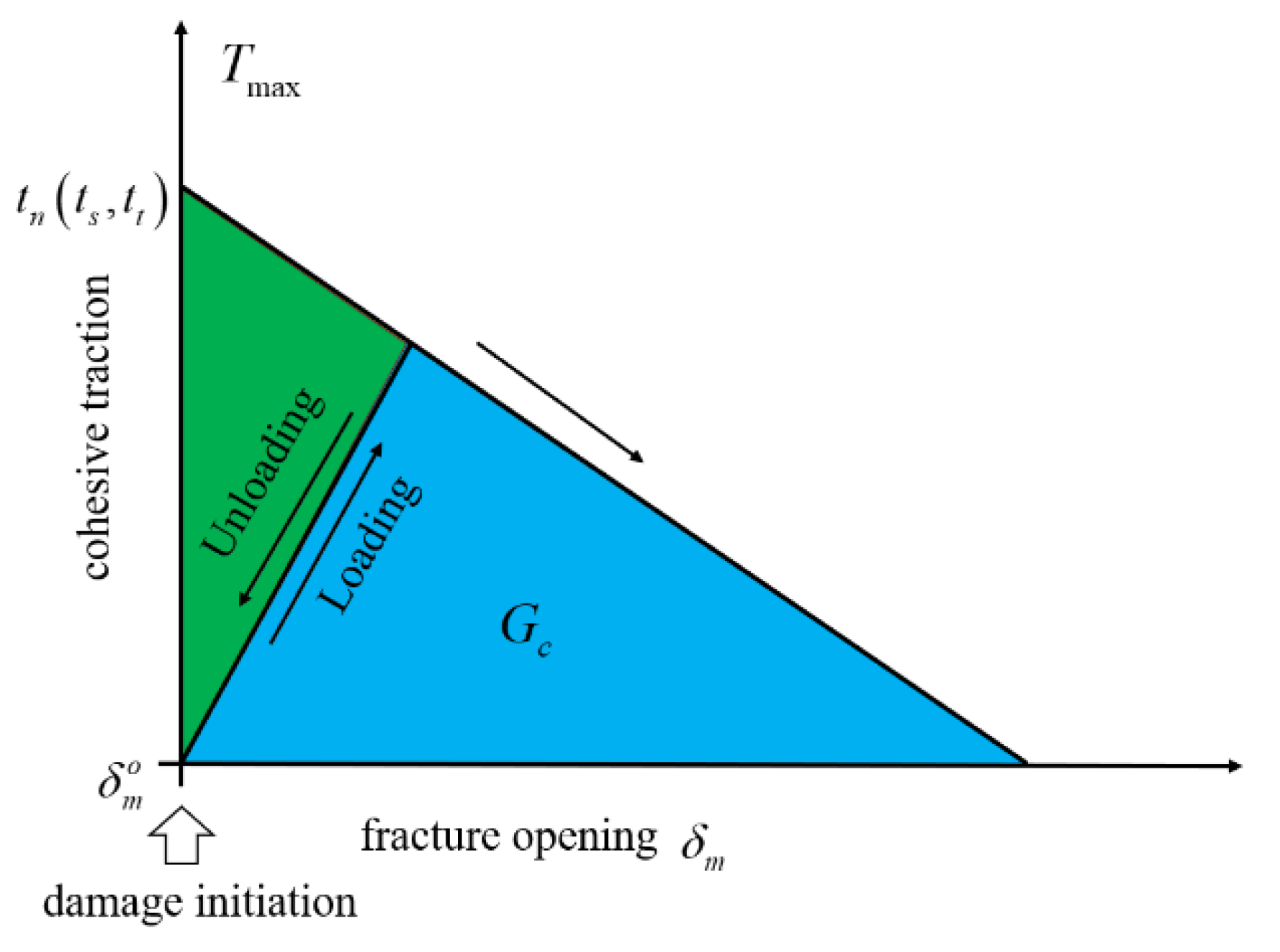
2.3. Fracture Propagation Criterion

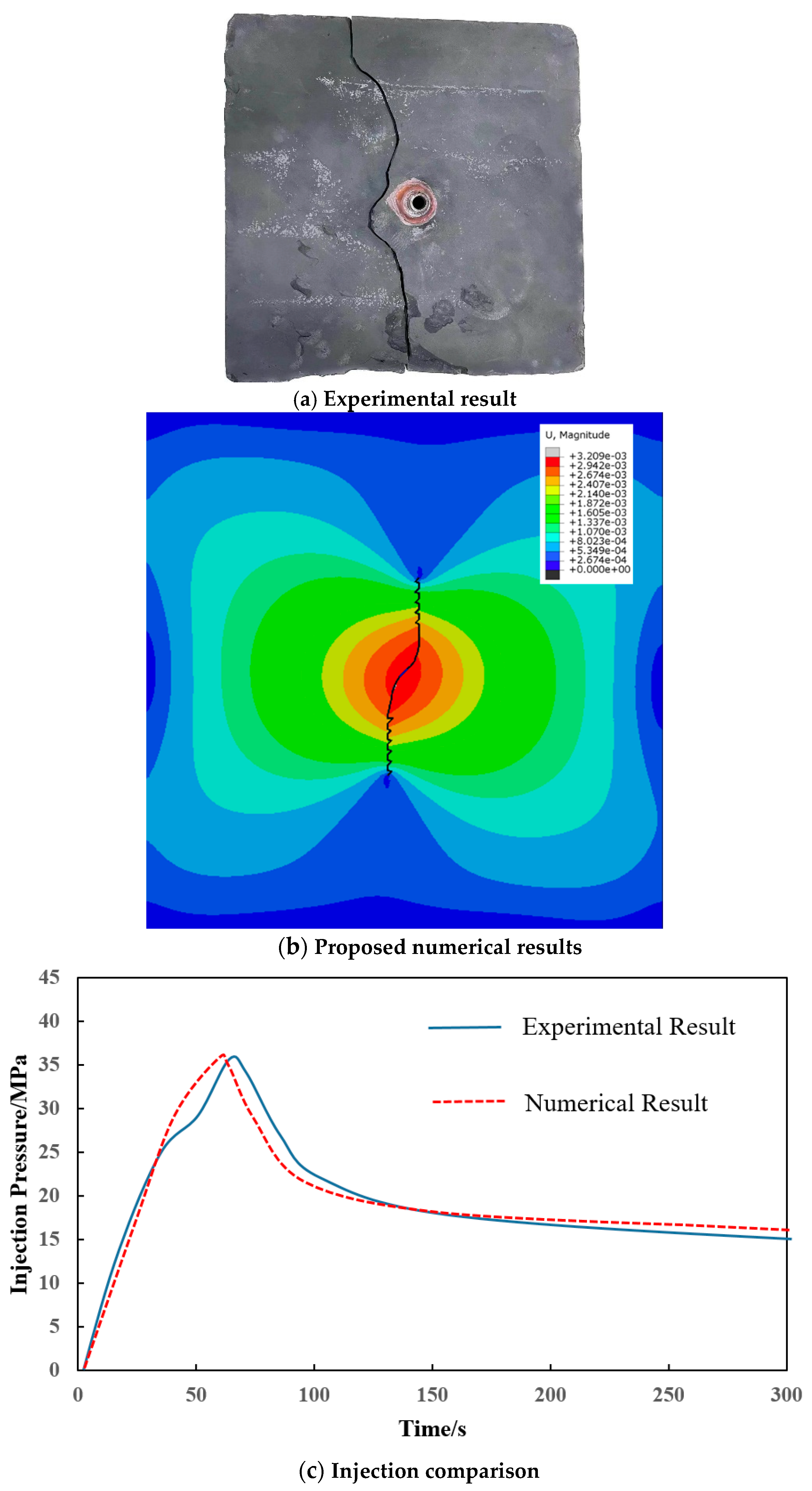
In the simulation, it was assumed that rock failure followed the linear elastic fracture mechanics characteristic; thus, the traction-separation criterion was used to describe rock failure during hydraulic fracturing. The traction-separation criterion is shown as Figure 1.

In the simulation, the second nominal principal stress criterion was introduced to describe the damage caused by fracturing fluid injection. In the simulation, both the tensile failure and shear failure were considered in the criterion [22], as follows:

$${\left\{{\displaystyle \frac{t_n}{t_n^0}}\right\}}^2+{\left\{{\displaystyle \frac{t_s}{t_s^0}}\right\}}^2=1$$

(6)

where $t_s^0$ and $t_n^0$ are the normal and shear strengths of an undamaged cohesive element, respectively; the symbol stands for the Macaulay bracket, and t_n and t_s stand for the normal and shear stress components, respectively.

The normal and shear stress components can be defined as follows:

$$t_n=\left\{\begin{array}{l}\left(1-D\right)T_n,T_n\ge 0\\ T_n,T_n<0\end{array}\right.$$

(7)

$$t_s=\left(1-D\right)T_s$$

(8)

$$t_t=\left(1-D\right)T_t$$

(9)

To characterize the damage caused by fracturing fluid injection, the scalar damage variable D was used to describe the entire fracturing process based on the mixed-mode energy theory. The area under the traction-separation curve represents the breaking energy. The damage variable for linear softening was shown as follows [23]:

$$D={\displaystyle \frac{U_m^f(U_m^{\max }-U_m^0)}{U_m^{\max }(U_m^f-U_m^0)}}$$

(10)

where $U_m^0$ is the effective displacement during the damage evolution; $U_m^f$ is the displacement when the material fails; and $U_m^{\max }$ is the maximum effective displacement during the loading.

For the fracture propagation, the Benzeggagh-Kenane (B-K) criterion was used to describe the fracture propagation, and the Benzeggagh-Kenane (B-K) criterion was shown as follows [24]:

$$G_n^C+\left(G_s^C-G_n^C\right){\left\{{\displaystyle \frac{G_s}{G_T}}\right\}}^{\eta }=G^C$$

(11)

G_c is the calculated total critical energy release rate due to mixed-mode failure; G_nc and G_sc are the critical energy release rates due to Mode I and Mode II fractures, respectively. The energy release rate of Mode I and Mode II cracks, G_n and G_s, are constants that depends on the type of material.

2.4. Verification

To verify the effectiveness of the proposed model, a single fracture propagation model was established and the results were compared with published numerical results [25]. In the simulation, the maximum horizontal principal stress and minimum horizontal principal stress were 41 MPa and 35 MPa, respectively; Young’s modulus and Possion’s rate were 36.4 GPa and 0.37; the injection rate was 3.5 m³/min; and the viscosity of the fracturing fluid was 10 mPa.s. From the comparison (Figure 2), it can be found that the injection pressure between the published numerical results and the proposed model had a good match, and the length error of the simulated fracture was only 3.4%. Thus, the effectiveness of the proposed model was verified.

3. Simulation and Discussion

3.1. Model Description

In the simulation, a 2D model with a length of 400 m and a width of 200 m was established, and the formation was discretized using the CPE4P (four-node pore pressure-stress) element, and the COH2D4P element was intersected between the CPE4P elements to describe the natural fracture present in the formation. The boundary of the established model was set as a fixed boundary because the stimulated area was much smaller than that of the whole model area, thus the displacement and stress on the boundary remained stable. In the model, the natural fracture angles were 30° and 150°, the initial natural fracture length was 0.5 m, the fracture density was 0.4 m, and the perforation direction was aligned with the direction of maximum horizontal stress. In the model, the minimum horizontal principal stress was kept stable, and the maximum horizontal principal stress was changed, thus the extension pressure of the hydraulic fracture did not have huge fluctuations. The other parameters were obtained from the Jimusar shale oilfield.

3.2. Discussion

3.2.1. Injection Rate of Fracturing Fluid on Fracture Propagation

To understand the effect of injection rate on fracture propagation in shale formations, different pumping rates of 8 m³/min, 10 m³/min, and 12 m³/min were simulated to investigate the fracture propagation. The other parameters in the modeling were shown in

Table 1. Input parameters of the numerical simulation.

Parameter	Value
Injection rate	8 m3/min
Young’s modulus	35 GPa
Poisson’s ratio	0.35
The minimum horizontal stress	36 MPa
The maximum horizontal stress	41 MPa
Fluid leak-off parameter	1 × 10−6 m3/Pa·s
Fluid viscosity	10 mPa·s
Formation porosity	0.15
Size of the study area	400 × 200 m

. Figure 3 indicates the fracture geometry under different pumping rates. From the simulation, it can be found that the hydraulic fracture propagation was not planar due to natural fractures. During hydraulic fracture propagation, the fracture propagation path was determined by two competing forces: one was the tendency to propagate along the weak plane generated by the natural fracture set, and the other was the tendency to propagate along the direction of the maximum principal stress. Generally speaking, the direction of natural fractures was inconsistent with the direction of in situ principal stress. Fracture propagation must balance these two forces, minimize fracturing energy, and find the path of least resistance, which was the main reason causing the zigzag path during hydraulic fracture propagation. It can be seen that the geometric shape of the crack was similar to the shape of an “elbow”, and the trajectory of the two hydraulic fracture wings was different. The deflection direction of the two hydraulic fracture wings on both sides was inclined to the X-axis. When the pumping rate increased to 10 m³/min, branch fractures were created, and the upper fracture propagated more easily with the increase in pumping rate. Meanwhile, it should be noted that the length of the created fractures had an obvious increase due to the amount of fracturing fluid also experiencing an increase, which was shown in Figure 4a. When the injection rate increased from 8 m³/min to 10 m³/min, it can be found that the total fracture length increased by 139.98%, from 105.3 m to 252.7 m, while it only increased by 40.12% when the injection rate increased from 10 m³/min to 12 m³/min. The breakdown pressure and extension pressure under different injection rates is shown in Figure 4b. From the simulation results, it can be concluded that breakdown pressures increased with the increase in pumping rate. When the injection rate was 8 m³/min, the breakdown pressure and average extension pressure were 44.6 MPa and 24.7 MPa, respectively. When the injection rate was 10 m³/min, the breakdown pressure and average extension pressure were 52.3 MPa and 35.2 MPa, respectively. When the injection rate was 12 m³/min, the breakdown pressure was close to that when the injection rate was 10 m³/min, while the extension pressure increased to 43.7 MPa. The main reason for this phenomenon was that as the injection rate increased, the number of branch fractures also increased, leading to a noticeable increase in breakdown pressure between 8 m³/min and 10 m³/min. However, when the injection rate increased to 12 m³/min, the number of branch fractures stabilized, resulting in little change in breakdown pressure. Furthermore, the tortuosity of the created fractures increased with the injection rate, directly causing an increase in extension pressure.

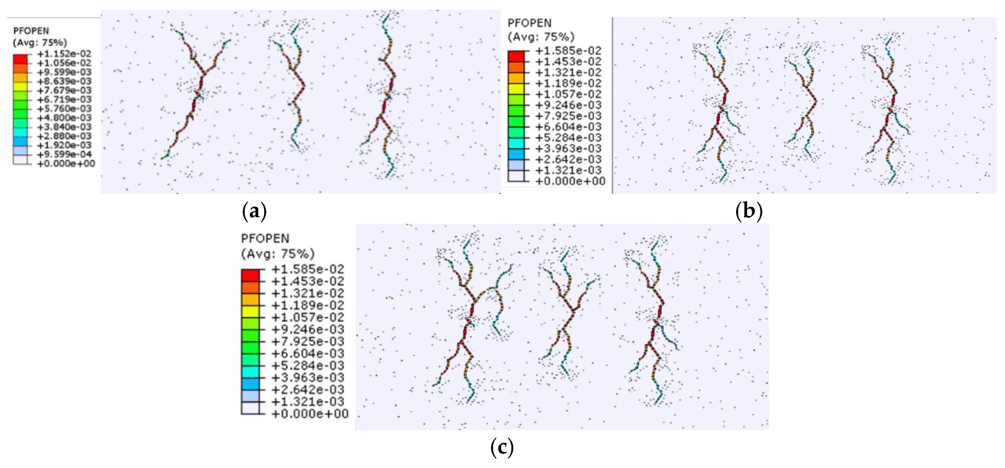
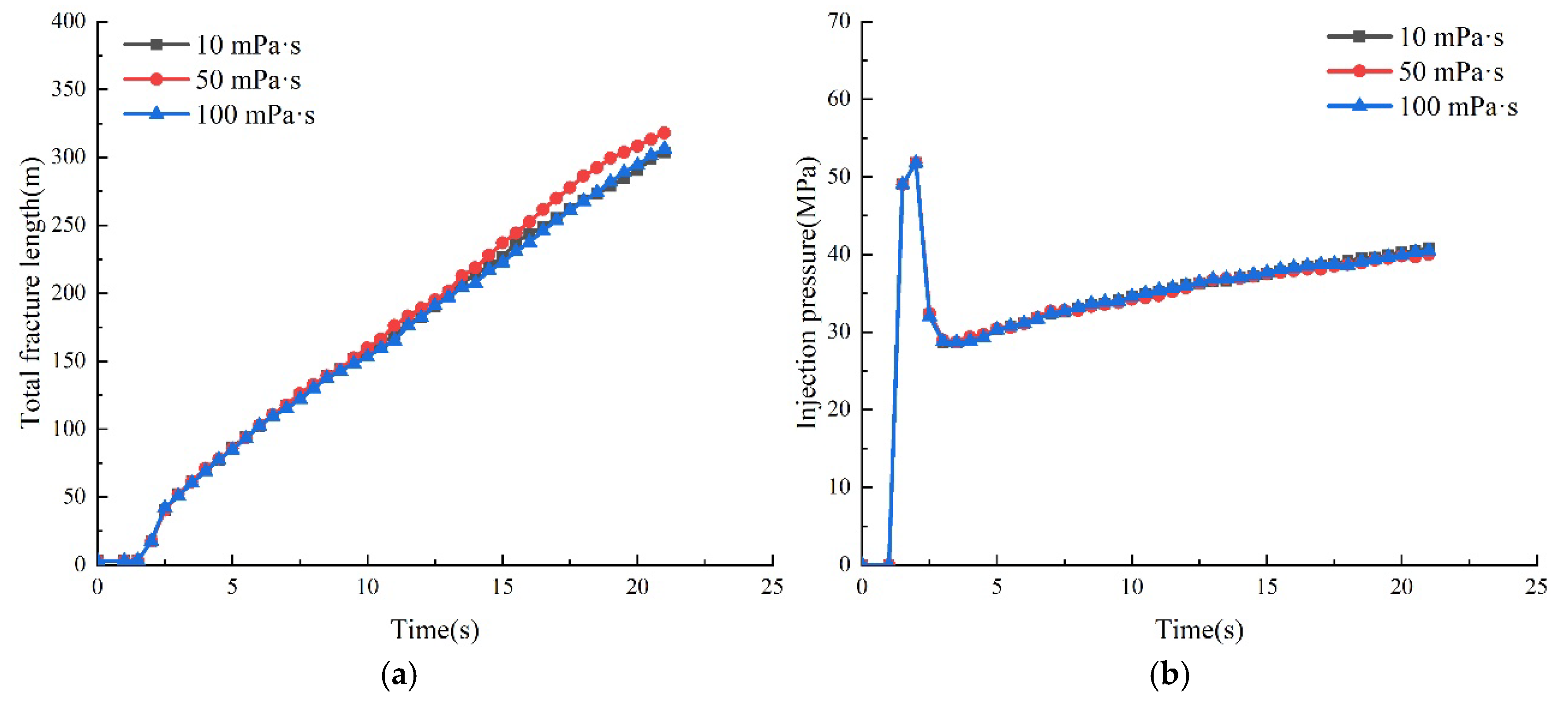
3.2.2. Influence of Viscosity of Fracturing Fluid on Fracture Propagation

To understand the effect of viscosity of fracturing fluid on fracture propagation in shale formations, different viscosities with 10 mPa·s, 50 mPa·s, and 100 mPa·s were simulated. To investigate the fracture propagation, the injection rate was 10 m³/min, the other parameters were as shown in Table 1. The simulation results (Figure 5) indicated that when the fracturing fluid viscosity increased from 10 mPa·s to 50 mPa·s, the total fracture length experienced a slight increase, and the tortuosity of the created fracture decreased obviously, the expansion path of the viscosity with 50 mPa·s tended to follow a straight line. When the viscosity continuously increased to 100 mPa·s, the tortuosity of the created fracture decreased further. It also can be found that the number of branch fractures decreased with the increase in viscosity of fracturing fluid. Figure 6 indicates that the total fracture length of the created fractures showed slight difference, and the breakdown pressure and extension pressure showed the same tendency. The main reason accounting for this was that under a low viscosity of fracturing fluid, the flow resistance was comparatively low, thus the fracturing fluid flowed much easier into the natural fracture, hence the number of branch fractures increased. With the increase in viscosity, the hydraulic fracture created crossed the natural fracture much easier, resulting in a straight fracture. From the simulation, when the fracturing fluid viscosity exceeded 50 mPa·s, the viscosity dominated the propagation direction of the fracture, allowing the hydraulic fracture to pass through the natural fracture. Meanwhile, although the extension pressure increased with the increase in tortuosity of the created fracture, the flow resistance of the created fracture also increased with higher fracturing fluid viscosity. Thus, while the straight fractures were created under high fracturing fluid viscosity, the extension pressure did not show an obvious decrease.

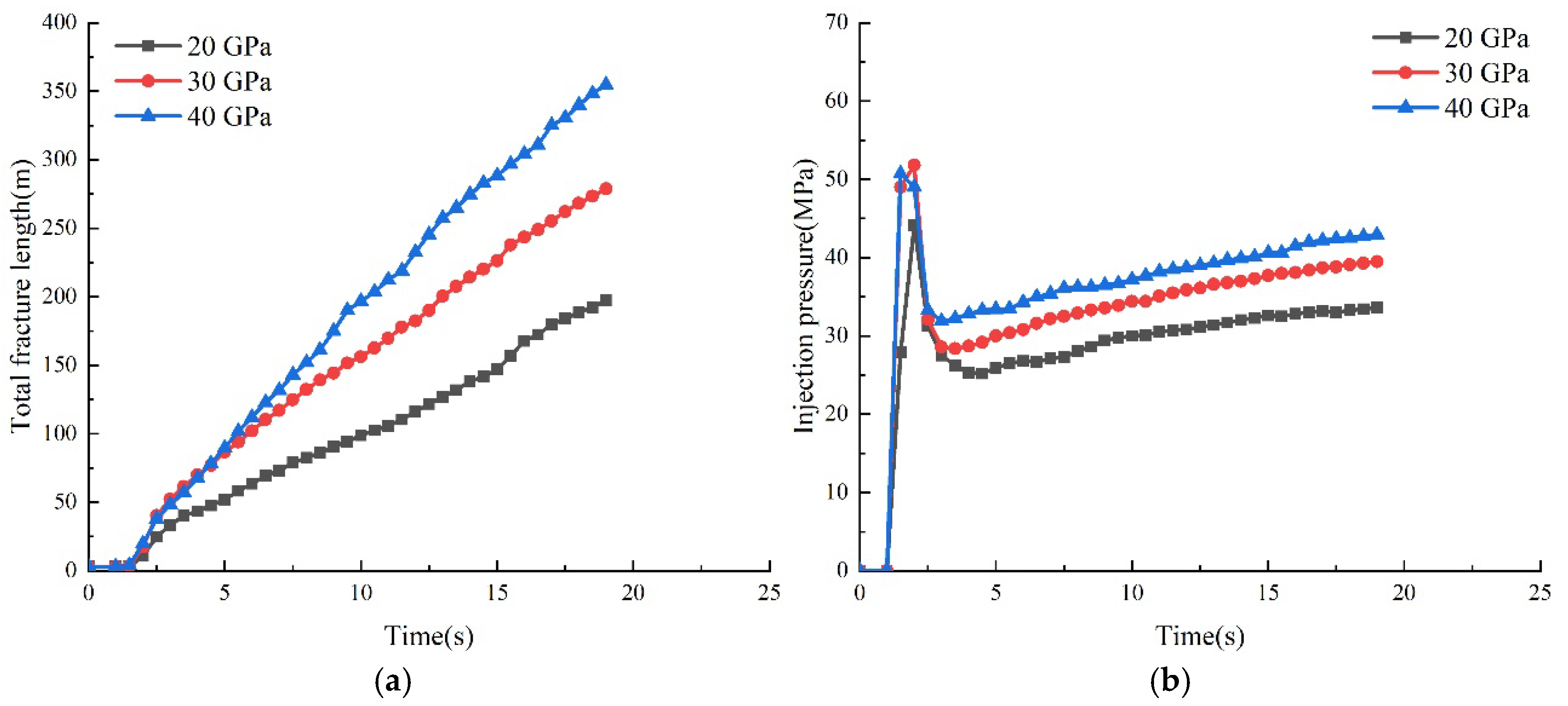
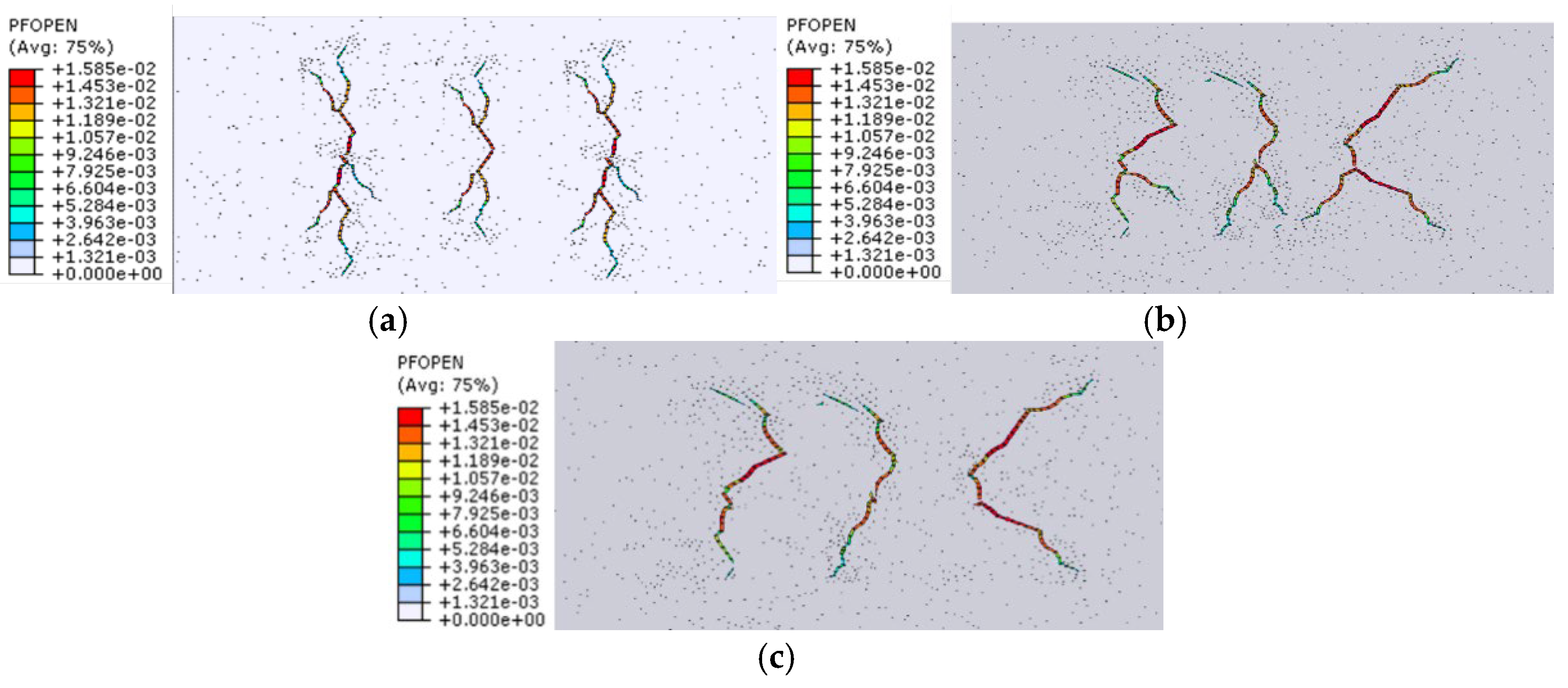
3.2.3. Influence of Elastic Modulus on Fracture Propagation

The elastic modulus of reservoir rock is an essential factor controlling fracture cracking and expansion. To further understand the effect of elastic modulus on fracture propagation, the elastic moduli of 20 GPa, 30 GPa, and 40 GPa were calculated. From the simulation, it was found that with an increase in elastic modulus, the number of branch fractures increased, the tortuosity of the created fractures increased significantly, and the total fracture length also increased. The simulation results (Figure 7) showed that the higher the elastic modulus was, the more complex the hydraulic fracture propagation was, and the easier it was to connect the natural fracture. As for the breakdown pressure and extension pressure, it can be found that both the breakdown pressure and extension pressure had a significant increase (Figure 8). The main reason accounting for this was that with the increase in elastic modulus, the strength difference between the rock matrix and natural fractures also increases, thus the interaction between hydraulic fractures and natural fractures changed from crossing to offset, thus more branch fractures were created when the hydraulic fracture propagated along the natural fracture under high elastic modulus. Meanwhile, with the increase in elastic modulus, the energy consumption for hydraulic propagation also increased, thus both the breakdown pressure and extension pressure increased.

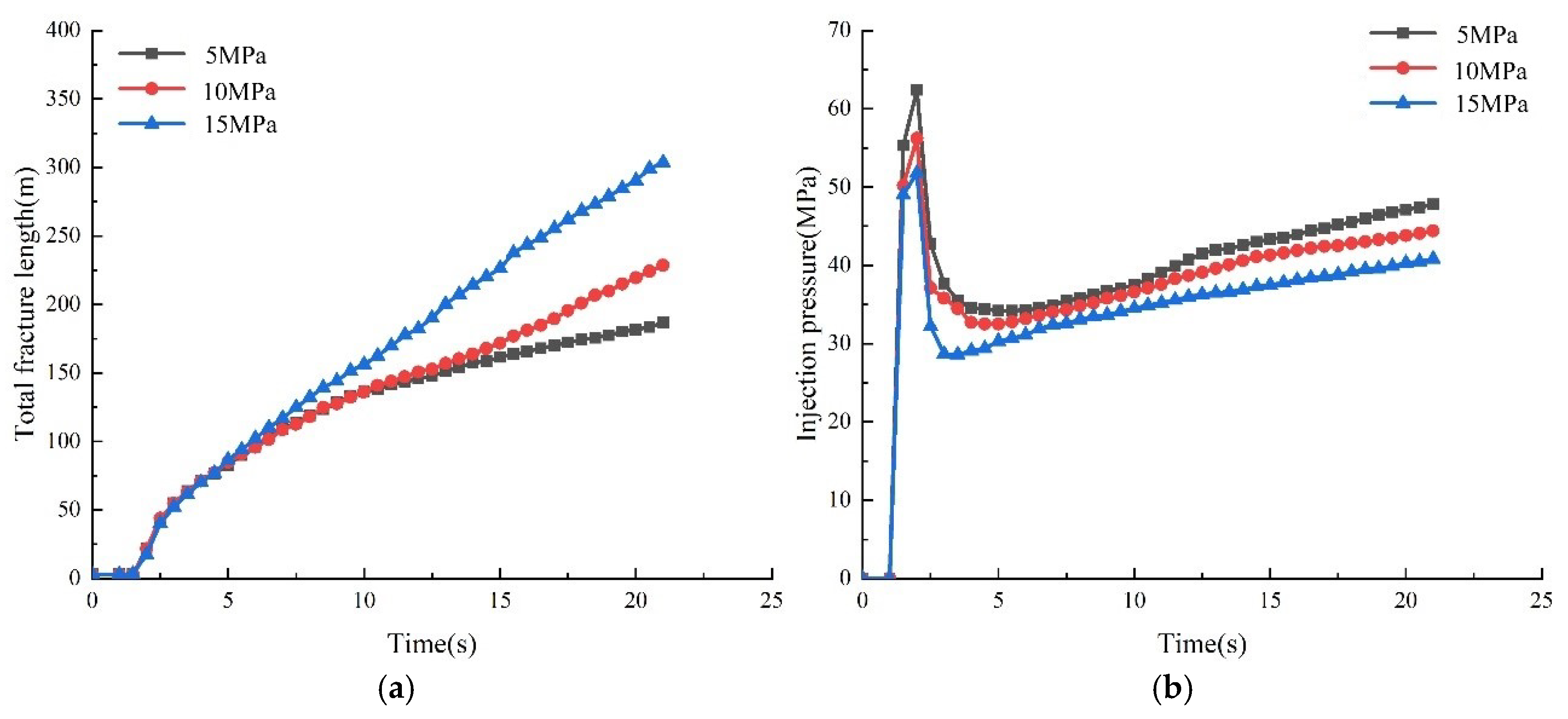
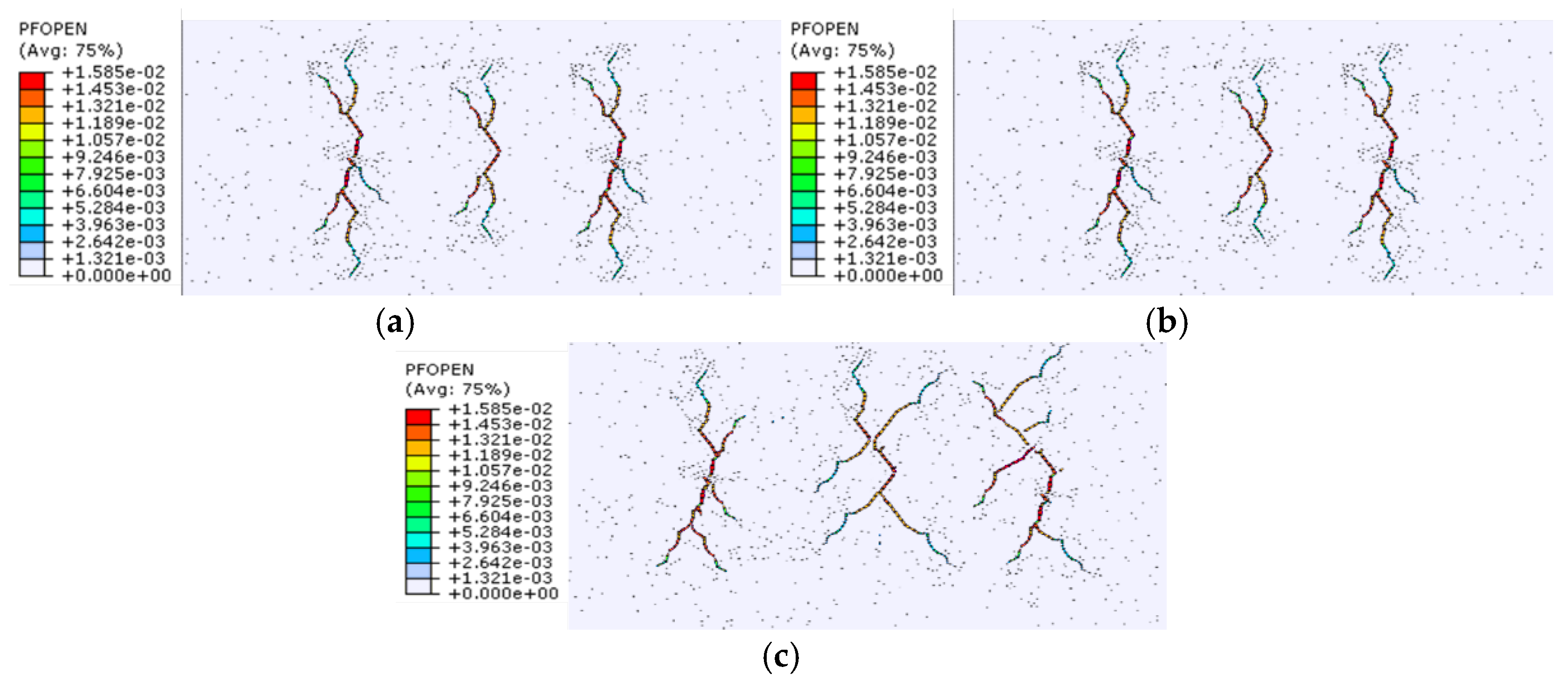
3.2.4. Influence of Horizontal Stress Differences on Fracture Propagation

In order to study the influence of horizontal stress differences on fracture propagation, the stress differences of 5 MPa, 10 MPa, and 15 MPa were simulated. In the simulation, to avoid the change of the minimum horizontal stress difference on fracture propagation, only the maximum horizontal stress difference was changed to obtain the target stress difference. The simulation (Figure 9) indicated that with an increase in horizontal stress difference, the number of branch fractures significantly increased, and the total length of the created fractures increased. Meanwhile, it also can be found that with an increase in horizontal stress difference, the fracture tended to propagate in a straight line, thus the tortuosity decreased. Under high stress differences (10 MPa and 15 MPa), it can be found that the direction of maximum horizontal stress was the propagation direction, while the propagation direction increased significantly when the stress difference was 5 MPa. The main reason was that under low stress differences, the simulated formation was comparatively uniform, thus many energy release channels were created when the fracturing fluid was injected, and the number of activated natural fractures also increased, so the number of branch fracture increased, and a hydraulic fracture with high tortuosity was created (Figure 10). With the increase of stress difference, the direction of maximum horizontal stress was the propagation direction, thus the number of branch fractures decreased, the number of activated natural fractures also decreased, the number of branch fracture also followed the same tendency.

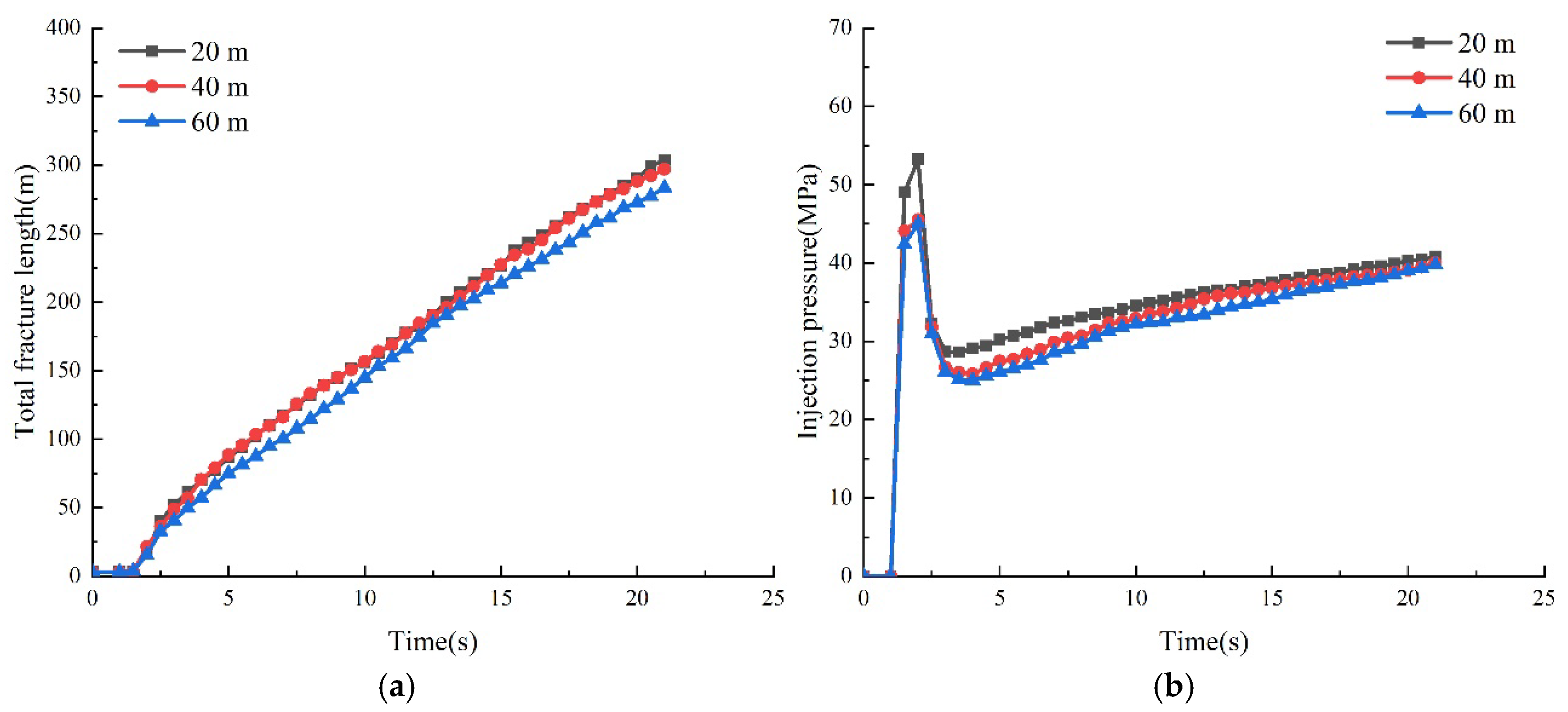
3.2.5. Influence of Cluster Space on Fracture Propagation

Cluster space was also an important factor affecting fracture propagation. To understand the effect of cluster space on fracture network creation, cluster spaces with 20 m, 40 m, and 60 m were simulated. From the simulation, it can be concluded that with an increase in cluster space, the number of branch fractures decreased, while the length of middle fractures increased (Figure 11). The main reason was that the “stress shadow” caused between fractures was more serious with the decrease in cluster space. When the cluster space was 20 m, more natural fractures were activated, thus more branch fractures were created during the hydraulic fracture propagation. While the “stress shadow” can also limit the propagation of middle fractures. The main reason was that the propagation resistance had an increase at the tip of the middle fractures, the length of the middle fractures was shorter than that of adjacent fractures. With the increase in cluster space, the “stress shadow” on fracture propagation was weakened, thus the number of activated natural fractures decreased, thus the branch fractures decreased, the tortuosity also decreased (Figure 12).

4. Conclusions

Hydraulic fracture has become the most important technology for shale oil and gas development. To further understand hydraulic fracture distribution in shale formations, a 2D hydraulic fracturing model was established which considered the natural fracture effect on fracture propagation. It was established based on the global cohesive element method and the influence of stress field, injection parameters and rock properties on fracture propagation were simulated. The conclusions were shown as follows:

(1) Natural fracture and stress field were the predominant factors affecting the hydraulic fracture propagation. Under low horizontal stress difference, the hydraulic fracture propagation was diverse, thus many branch fractures were created, and the tortuosity of hydraulic fractures also increased due to the increase in the activated natural fracture.

(2) Low viscosity of the fracturing fluid and high injection rates were helpful for creating complex fracture networks. The main reason was that low flow resistance of the low-viscosity fracturing fluid made the natural fractures to be activated more, thus the hydraulic fracture had a difference in propagation trajectory. High injection rate can provide high net pressure which was helpful in activating the natural fracture.

(3) With the increase in elastic modulus, the number of branch fractures increased, and the tortuosity of the created fractures increased significantly. The main reason was that the high difference in strength between the rock matrix and the natural fracture can change the interaction between a hydraulic fracture and a natural fracture from crossing to offset, which activated the natural fracture more, thus more branch fractures were created.

References

1. Zeng, J.; Wang, X.; Guo, J.; Zeng, F.; Zhang, Q. Composite linear flow model for multi-fractured horizonal wells in tight sand reservoirs with the threshold pressure gradient. J. Pet. Sci. Eng. 2018, 165, 890–912. [Google Scholar] [CrossRef]
2. Wang, Z.L.; Lou, Y.; Pan, J.P. China’s Oil & gas resources exploration and development and its prospect. Explor. Prod. 2017, 25, 1–6. [Google Scholar]
3. Wang, K.; Zhang, H.L.; Zhang, R.H.; Wang, J.P.; Dai, J.S.; Yang, X.J. Characteristics and influencing factors of ultra-deep shale reservoir structural fracture: A case study of Keshen-2 gas field, Tarim Basin. Acta Petrol. Sin. 2016, 37, 714–727. [Google Scholar]
4. Yang, T.; Zhang, G.S.; Liang, K.; Zheng, M.; Guo, B.J. The exploration of global shale gas and forecast of the development tendency in China. Strateg. Study CAE 2012, 14, 64–68. [Google Scholar]
5. Zeng, L.B.; Ke, S.Z.; Liu, Y. Research Methods of Low Permeability Oil and Gas Reservoir Fractures; Petroleum Industry Press: Beijing, China, 2010; pp. 1–187. [Google Scholar]
6. Olson, J.E.; Laubach, S.E.; Eichhubl, P. Estimating natural fracture producibility in tight gas sandstones, coupling diagenesis with geomechanical modeling. Lead. Edge 2010, 29, 1494–1499. [Google Scholar] [CrossRef]
7. Zeng, L.; Liu, W.; Li, J.; Zhu, L.; Weng, J.; Yue, F.; Zu, K. Natural fractures and their influence on shale gas enrichment Sichuan Basin, China. J. Pet. Sci. Eng. 2016, 30, 1–9. [Google Scholar] [CrossRef]
8. Liu, W.; Zeng, L.; Zhang, B.; Miao, F.; Lyu, P.; Dong, S. Influence of natural fractures on gas accumulation in the Upper Triassic tight gas sandstones in the northwestern Sichuan Basin, China. Mar. Pet. Geol. 2017, 83, 60–72. [Google Scholar] [CrossRef]
9. Fisher, M.K.; Wright, C.A.; Davidson, B.M.; Steinsberger, N.P.; Buckler, W.S.; Goodwin, A.; Fielder, E.O. Integrating fracture mapping technologies to optimize stimulations in the Barnett shale. In Proceedings of the SPE Annual Technical Conference and Exhibition, San Antonio, TX, USA, 29 September–2 October 2002. SPE-77411. [Google Scholar]
10. Zheng, H.; Liao, R.; Cheng, N.; Shi, S.; Liu, D. Study of mechano-chemical effects on the morphology of hydraulic fractures. J. Pet. Sci. Eng. 2021, 206, 109031. [Google Scholar] [CrossRef]
11. Maxwell, S.C.; Urbanci, K.T.; Steinsberger, N.P.; Zinno, R. Microseismic imaging of hydraulci fracture complexity in the barnett shale. In Proceedings of the SPE Annual Technical Conference and Exhibition, San Antonio, TX, USA, 29 September–2 October 2002. SPE-77440. [Google Scholar]
12. Perkins, T.K.; Kern, L.R. Width of hydraulic fractures. J. Pet. Technol. 1961, 13, 937–949. [Google Scholar] [CrossRef]
13. Gu, H.; Weng, X. Criterion for fractures crossing frictional interfaces at nonorthogonal angles. In Proceedings of the 44th US Rock Mechanics Symposium and 5th US-Canada Rock Mechanics Symposium, Salt Lake City, UT, USA, 27–30 June 2010. ARMA-10-198. [Google Scholar]
14. Tan, P.; Jin, Y.; Han, K.; Hou, B.; Chen, M.; Guo, X.; Gao, J. Analysis of hydraulic fracture initiation and vertical propagation behavior in laminated shale formation. Fuel 2017, 206, 482–493. [Google Scholar] [CrossRef]
15. Zhang, H.; Sheng, J.J. Numerical simulation and optimization study of the complex fracture network in naturally fractured reservoirs. J. Pet. Sci. Eng. 2020, 195, 107726. [Google Scholar] [CrossRef]
16. Rui, Z.; Guo, T.; Feng, Q.; Qu, Z.; Qi, N.; Gong, F. Influence of gravel on the propagation pattern of hydraulic fracture in the conglomerate reservoir. J. Pet. Sci. Eng. 2018, 165, 627–639. [Google Scholar] [CrossRef]
17. Zhang, G.; Sun, S.; Chao, K.; Niu, R.; Liu, B.; Li, Y.; Wang, F. Investigation of the nucleation, propagation and coalescence of hydraulic fractures in conglomerate reservoirs using a coupled fluid loe-DEM approach. Powder Technol. 2019, 354, 301–313. [Google Scholar] [CrossRef]
18. Chen, M.; Sun, Y.; Fu, P.; Carrigan, C.R.; Lu, Z.; Tong, C.H.; Buscheck, T.A. Surrogate-based optimization of hydraulic fracture in pre-existing fracture networks. Comput. Geosci. 2013, 58, 69–79. [Google Scholar] [CrossRef]
19. Wang, H.Y. Hydraulic fracture propagation in naturally fractures reservoirs: Complex fracture or fracture networks. J. Nat. Gas Sci. Eng. 2019, 68, 102911. [Google Scholar] [CrossRef]
20. Wei, Y.S.; Wang, J.L.; Yu, W.; Qi, Y.D.; Miao, J.J.; Yuan, H.; Liu, C.X. A smart productivity evaluation method for shale gas wells based on 3D fractal fracture network model. Pet. Explor. Dev. 2021, 48, 787–796. [Google Scholar] [CrossRef]
21. Wan, X.C.; Rasouli, V.; Damjance, B.; Yu, W.; Xie, H.; Li, N.; Rabiei, M.; Miao, J.; Liu, M. Coupling of fracture model with reservoir to simulate shale gas production with complex fractures and nanopores. J. Pet. Sci. Eng. 2020, 193, 107422. [Google Scholar] [CrossRef]
22. Sobhaniaraghn, B.; Mansur, W.J.; Peter, F.C. Three-dimensional investigation of multiple stage hydraulic fracturing in unconventional reservoirs. J. Pet. Sci. Eng. 2016, 146, 1063–1078. [Google Scholar] [CrossRef]
23. Khoei, A.R.; Vahab, M.; Ehsani, H.; Rafieerad, M. XFEM modeling of large plasticity deformation; a convergence study on various blending strategies for weak discontinuities. Eur. J. Comput. Mech. 2015, 24, 79–106. [Google Scholar] [CrossRef]
24. Hanks, C.L.; Lorenz, J.; Teufel, L.; Krumhardt, A.P. Lithologic and structural controls on natural fracture distribution and behavior within the Lisburne Group, northeastern Brooks Range and North Slope subsurface, Alaska. AAPG Bull. 1997, 81, 1700–1720. [Google Scholar]
25. Wang, H.; Sharma, M.M. New variable compliance method for estimating closure stress and fracture compliance from DFIT data. In Proceedings of the SPE Annual Technical Conference and Exhibition, San Antonio, TX, USA, 9–11 October 2017. SPE-187348. [Google Scholar]
Figure 1. Traction-separation relationship for fracture initiation.
Processes 12 02630 g001
Figure 2. (a) Published numerical results. (b) Proposed model. (c) Injection comparison. Simulation results comparison between the published results and the proposed model.
Processes 12 02630 g002
Figure 3. (a) 8.0 m3·min−1. (b) 10.0 m3·min−1. (c) 12.0 m3·min−1. Distribution of hydraulic fracture under different injection rate.
Processes 12 02630 g003
Figure 4. (a) Comparison of the total length of fractures. (b) Injection pressure comparison. Changes of total fracture length and fracture pressure at different injection rate.
Processes 12 02630 g004
Figure 5. (a) 10 mPa·s. (b) 50 mPa·s. (c) 100 mPa·s. Distribution of hydraulic fracture under different fracturing fluid viscosity.
Processes 12 02630 g005
Figure 6. (a) Comparison of the total length of cracks. (b) Rupture pressure comparison chart. Changes of total fracture length and injection pressure under different fracturing fluid viscosity.
Processes 12 02630 g006
Figure 7. (a) 20 GPa. (b) 30 GPa. (c) 40 GPa. Distribution of hydraulic fracture under different elastic modulus.
Processes 12 02630 g007
Figure 8. (a) Comparison of the total length of cracks. (b) Rupture pressure comparison chart. Changes of total fracture length and injection pressure under different elastic modulus.
Processes 12 02630 g008
Figure 9. (a) 5 MPa. (b) 10 MPa. (c) 15 MPa. Distribution of hydraulic fractures under different stress differences.
Processes 12 02630 g009
Figure 10. (a) Comparison of the total length of cracks. (b) Rupture pressure comparison chart. Changes in total fracture length and fracture pressure under different horizontal stress differences.
Processes 12 02630 g010
Figure 11. (a) 20 m. (b) 40 m. (c) 60 m. Distribution of hydraulic fractures under different cluster spaces.
Processes 12 02630 g011
Figure 12. (a) Comparison of the total length of cracks. (b) Rupture pressure comparison chart. Changes in total fracture length and fracture pressure under different cluster spaces.
Processes 12 02630 g012