Assessment of the Influences of Numerical Models on Aerodynamic Performances in Hypersonic Nonequilibrium Flows

Abstract

In this paper, the aerodynamic performances including shock wave standoff distance (SSD) and heat flux of ELECTRE vehicle at 53.3 km and 4230 m/s for several types of numerical models are investigated. The numerical models include thermal equilibrium/nonequilibrium (1T/2T) assumption, three surface boundary conditions (no-slip/non-catalytic, slip/non-catalytic, slip/fully-catalytic), four chemical kinetic models (DK, Park, Gupta, and No Reaction (NR)) and two controlling temperatures (T_tr^0.7T_ve^0.3, T_tr^0.5T_ve^0.5). The results show that the chemical kinetic model significantly affects the SSD, and its value gradually decreases with the increase in chemical reaction rate. The SSD predicted by the NR model is 20.7% larger than that of the Park model. The SSD is also affected by the proportion of vibro-electronic temperature (T_ve) in the controlling temperature, and the higher the proportion, the larger the SSD. Regarding the heat flux, the catalytic surface setting is crucial, where the value predicted by the fully-catalytic model is 62.2% higher than that by the non-catalytic model. As the chemical reaction rate of Gupta, DK, and Park models increases sequentially, the calculated heat flux decreases in turn. The heat flux predicted by the 2T model is lower than that by the 1T model, and the higher T_ve proportion in the controlling temperature, the smaller the heat flux. The fundamental reason is that the trans-rotational convective heat flux of the 2T model is much lower than that of the 1T model, and the trans-rotational convective heat flux decreases with an increase in the T_ve proportion.

1. Introduction

During the hypersonic flight of vehicles, a generous kinetic energy is converted into high temperature, which is sufficiently high to result in serious physicochemical phenomena, such as vibrational excitation and chemical reactions. At a high altitude (40–100 km), the relaxation times of the internal energy modes and chemical reactions are greatly prolonged due to the rarefied environment; thus, nonequilibrium characteristics appear easily [1]. The discrete particle model can accurately describe the nonequilibrium characteristics from the perspective of physical mechanism [2], but expensive calculations prevent its application at a low Knudsen number (Kn).

The computational fluid dynamics (CFD) method has high computational efficiency [3]. However, conventional N-S equations are recommended for the continuum flow (Kn < 0.001), regarding that different internal energy modes are always in equilibrium and that chemical reactions are only related to local pressure and temperature. Researchers proposed the nonequilibrium Navier–Stokes (N-S) equations [4,5] to expand the application range of the CFD method. In addition, researchers had reached a consensus that the nonequilibrium N-S equations can be used in the range of 0.001 < Kn < 0.1 [6]. Compared with conventional N-S equations, the relaxation processes of chemical reactions and/or various internal energy modes are considered in nonequilibrium N-S equations. The setting of numerical models is the key to the accuracy of prediction results, such as thermal equilibrium (one-temperature model, 1T) or thermal nonequilibrium (Two-temperature model, 2T [5]), chemical kinetic models, controlling temperatures, and boundary conditions.

A lot of nonequilibrium model validations are conducted by researchers through comparing the flight data or ground experiments. The ELECTRE capsule flight experiments were performed in 1971 in Europe [7], providing the related data of aerodynamic heat, force, and wall temperature during the ELECTRE reentry. Muylaert [7] first simulated the ELECTRE at an altitude of 53.3 km and Mach number (Ma) of 13 with the 2T and 5-species Dunn–Kang (DK) models. It is found that the distribution of heat flux on the ELECTRE surface exhibits a good agreement with the flight data. Subsequently, this case has been performed by Hao [8] and Niu [9] using the 2T 5-species Gupta model, as well as Kim [10] applying the 2T 11-species Kim2020 model. The heat fluxes predicted by the above models are not obviously different, and all are in good agreement with the flight data. A set of ground experiments of double cone and hollow cylinder flare were performed by Calspan-University of Buffalo Research Center (CUBRC) [11,12] and Holden [13]. In the early stages, researchers focused on the influence of vibrational nonequilibrium on the surface properties, in which pure Nitrogen without reactions is applied. It was found that, when considering the vibrational nonequilibrium, the accuracy of the predictions can be further improved [14,15]. Machlean [12] compared the surface properties predicted by different hypersonic solvers with experiment data. It is revealed that the CFD simulations are very consistent with each other except for the specific instances. Moreover, all predicted results are larger than the experiment data. However, the details of nonequilibrium models used in these hypersonic solvers were not presented. Hao [16] simulated the double cone with the 2T Park 93 and 2T CVDV models and drew the same conclusions as Machlean. Kianvashrad [17] calculated the hollow cylinder flare with the perfect gas and 2T Park85 models and found that the values of surface properties predicted by the perfect gas model are more consistent with the experiment data at total enthalpies of 10.43 and 15.54 MJ/kg.

The influences of chemical kinetic models on aerodynamic performances have been widely discussed by researchers. Wang [18] assessed the heat fluxes of ELECTRE, Apollo, and Space Shuttle Orbiter in various freestreams with the DK, Gupta, Park 87, and Park 91 models. It is revealed that the complicated geometry is highly sensitive to the choice of chemical kinetic model. Niu [9] studied the performances for three chemical kinetic models and two controlling temperatures regarding the species formation over the BSUV and RAM C-II vehicles. It is found that both the reaction rate model and the controlling temperature have a distinctive influence on the species concentration. Holloway [19] investigated the influences of the chemical reaction rate (nonequilibrium, equilibrium, and frozen models) on surface properties over a double cone and concluded that the heat flux is more sensitive to thermochemistry models than the aerodynamic force. Dobrov [20] found that using different chemical models did not significantly affect the species concentration and friction coefficient, but apparently did affect the shock standoff distance.

In addition, the settings of surface boundary conditions are vital for the predictions of aerodynamic performances in hypersonic flows. The slip boundary conditions, including the velocity slip and temperature jump of the gas near the surface, should be considered in a rarefied gas [21]. Lofthouse [22] investigated the surface properties of a cylinder in the Mach 10 and 25 flows of argon gas with Kn ranging from 0.002 to 0.25. It found that the errors under no slip conditions are larger than those under slip conditions, especially for a large Kn. The catalytic wall is another common boundary condition in hypersonic flows, which takes the recombination reactions on the surface into account [23]. MacLean and Holden [24] conducted experiments of the cylinder and 70-degree sphere-cone models at CUBRC using LENS facilities, and compared the results with the CFD predictions. It revealed that the measured heat flux data are higher than those predicted with a non-catalytic wall. Research [25,26] has shown that the heat flux predicted by the fully-catalytic wall is much larger than that by the non-catalytic wall. The setting of catalytic efficiency is critical to the heat flux value, Needels [27] found that the heat flux of catalytic efficiency of 0.1 is an approximately 45% increase relative to the non-catalytic heat flux value. Yang [28] evaluated the catalytic efficiencies of oxygen and nitrogen atoms through CFD analysis based on the Park and Cheung experiments and obtained that the efficiencies of oxygen and nitrogen atoms on the copper oxide surface at room wall temperature were 0.0045 and 0.003, respectively.

The references mentioned above focused on the influences of a single type of numerical model (chemical kinetic models, boundary conditions, or controlling temperatures) on aerodynamic performances, which cannot quantitatively present the effects of different types of numerical models on the aerodynamic performances. In addition, the reasons for different prediction results for aerodynamic performances with various numerical models are not explained clearly. In this paper, based on the ELECTRE flight experiments [6], we systematically evaluated the impact of several types of numerical models on the surface heat flux and the shock wave standoff distance and explained the fundamental reason why these numerical models affect the value of aerodynamic heating. The work refers to the flight experiment data of hypersonic vehicles, aiming to improve the prediction accuracy of aerodynamic performances of hypersonic vehicles by comprehensively analyzing the effects of different types of numerical models, and provide effective reference for vehicle design work.

The content of this paper is organized in the following order. Section 1 is the introduction. Section 2 describes the numerical approach in detail, including nonequilibrium N-S equations, wall boundaries, and chemical kinetic models. Section 3 presents the physical model of ELECTRE vehicle and boundary conditions, and it conducts grid convergence analysis. Section 4 presents the flow features and the results of SSD and heat flux under different numerical models and discusses deeply the influence of numerical models on the heat flux. Section 5 summarizes the main conclusions of this paper.

2. Numerical Approach

2.1. Nonequilibrium N-S Equations

According to the hierarchy of the relaxation times for the chemical reactions (τ_c), vibrational excitation (τ_v), rotational excitation (τ_r) and translation (τ_t): τ_t < τ_r < τ_v < τ_c [29], the chemical nonequilibrium is most likely to occur, and then it should be a vibrational nonequilibrium in a rarefied gas environment. The chemical nonequilibrium is taken into account in both 1T and 2T models. The difference is that, for the 1T model, all the internal energy modes are assumed to be in equilibrium with the translational model, whereas the relaxation process of vibrational energy is considered in the 2T model. Specifically, for the 2T model, one temperature is to characterize the translational and rotational energies, and the other temperature is to denote the vibrational, electron translation, and electronic excitation energies [5]. Moreover, regarding the 1T model, the continuity equation for the individual species (Equation (1)), the momentum equation (Equation (2)), and the total energy equation (Equation (3)) are required. For the 2T model, not only are Equations (1)–(3) necessary, but the vibrational-electronic energy equation (Equation (4)) is added [30]. The vibrational energies of different molecules in a mixture are assumed to be tightly coupled with each other; thus, the single vibrational energy equation (Equation (4)) for the system is used.

$${\displaystyle \frac{\partial {\rho }_s}{\partial t}}+{\displaystyle \frac{\partial }{\partial x_j}}\left({\rho }_s{u}_j+J_{s,j}\right)={\dot{\omega }}_s$$

(1)

$${\displaystyle \frac{\partial }{\partial t}}\left(\rho u_i\right)+{\displaystyle \frac{\partial }{\partial x_j}}\left(\rho u_i{u}_j+p{\delta }_{ij}-{\tau }_{ij}\right)=0$$

(2)

$${\displaystyle \frac{\partial E}{\partial t}}+{\displaystyle \frac{\partial }{\partial x_j}}\left((E+p)u_j-{\tau }_{ij}{u}_i+q_j+{\displaystyle \sum _{s=1}^{ns}{J}_{s,j}}{h}_s\right)=0$$

(3)

$${\displaystyle \frac{\partial E_{ve}}{\partial t}}+{\displaystyle \frac{\partial }{\partial x_j}}\left(E_{ve}{u}_j+q_{ve,j}+{\displaystyle \sum J_{s,j}{h}_{ve,s}}\right)={\displaystyle \sum {\rho }_s\frac{e_{ve,s}(T_{tr})-e_{ve,s}(T_{ve})}{{\tau }_{V-T,s}}}+{\displaystyle \sum {\dot{\omega }}_s{E}_{ve,s}}$$

(4)

where ${\rho }_s$ is the density of species s (kg/m³); $u_i$ and $u_j$ are the velocity vectors at i and j direction (m/s), respectively; p is the pressure (Pa); E and E_ve are the total and vibro-electronic energies per unit volume (J/m³), respectively; e_ve,s(T_tr) and e_ve,s(T_ve) are the vibrational energies per unit mass of species s (J/kg); J_s,j is the mass diffusion flux of species s (kg/(m²·s)); $q_j$ and $q_{ve,j}$ are the total and vibro-electrical heat conduction vectors (J/(m²·s)), respectively; h_s and h_ve,s are the total and vibro-electronic enthalpies (J/kg), respectively; δ_ij is the Kronecker delta (dimensionless); ${\tau }_{V-T,s}$ is the average relaxation time between the translational and vibrational energies of molecule s (s); $\dot{{\omega }_s}$ is the net mass production of species s (kg/(m³·s)).

The chemical source term, ${\dot{\omega }}_s$, can be expressed as [31]

$${\dot{\omega }}_s=M_s{\displaystyle \sum _{r=1}^{nr}\left(v_{s,r}^{″}-v_{s,r}^{\prime }\right)}\left[k_{f,r}{\displaystyle \prod _{s=1}^{ns}{\left(\frac{{\rho }_s}{M_s}\right)}^{v_{s,r}^{\prime }}}-k_{b,r}{\displaystyle \prod _{s=1}^{ns}{\left(\frac{{\rho }_s}{M_s}\right)}^{v_{s,r}^{″}}}\right]$$

(5)

where $v_{s,r}^{″}$ and $v_{s,r}^{\prime }$ are the forward and backward stoichiometric coefficients of species s in the reaction r, respectively; $k_{f,r}$ and $k_{b,r}$ represent the forward and backward reaction rate coefficients in the reaction r (m³/(s·mol)), respectively. M_s is the molecular weight of species s (kg/mol).

The viscous stress tensor, τ_ij, is written as [32]

$${\tau }_{ij}=\mu \left({\displaystyle \frac{\partial u_i}{\partial x_j}}+{\displaystyle \frac{\partial u_j}{\partial x_i}}\right)-{\displaystyle \frac{2}{3}}\mu {\displaystyle \frac{\partial u_k}{\partial x_k}}{\delta }_{ij}$$

(6)

where μ is the dynamic viscosity (kg/(m·s)).

The heat conduction vector, q_j, is assumed to follow the Fourier heat law. The total heat conduction vector is written as Equation (7) for the 1T model and is written as Equation (8) for the 2T model [18].

$$q_j=-\kappa {\displaystyle \frac{\partial T}{\partial x_j}}$$

(7)

$$q_j=q_{tr,j}+q_{ve,j}=-{\kappa }_{tr}{\displaystyle \frac{\partial T_{tr}}{\partial x_j}}-{\kappa }_{ve}{\displaystyle \frac{\partial T_{ve}}{\partial x_j}}$$

(8)

where κ, κ_tr, and κ_ve are the total, trans-vibrational, and vibro-electronic thermal conductivities (J/(m·s·K)) for a mixture, respectively.

The mass diffusion flux for heavy species can be calculated by using the modified Fick’s model [33], written as

$$J_{s\ne e,j}=-\rho D_s{\displaystyle \frac{\partial Y_s}{\partial x_j}}-Y_s{\displaystyle \sum _{r\ne e}(-\rho D_r\frac{\partial Y_r}{\partial x_j}})$$

(9)

where D_s and D_r are effective diffusion coefficients of species s and r in a mixture (m²/s), respectively.

For a mixture, the average relaxation time between the translational and vibrational energies for molecule s, can be expressed by

$${\tau }_{s,V-T}={\displaystyle \frac{{\displaystyle \sum _{r=mol}{X}_r}}{{\displaystyle \sum _{r=mol}{X}_r}/{\tau }_{s-r,V-T}}}$$

(10)

where the relaxation time between the translational and vibrational energies for molecules s and r (s), τ_s-r,V-T, is calculated by the Millikan–White–Park model [34].

The viscosity and the thermal conductivities presented in the above equations are applied in a mixture, which can be calculated by individual species with appropriate mixing rules. The viscosity and the thermal conductivities of individual species are obtained from the Blottner [35] and Eucken models [32], respectively. The Wilke–Armaly–Sutton mixing rule [36] is used in this paper. The effective diffusion coefficient is calculated by the binary diffusion coefficient [33].

2.2. Wall Boundary Conditions

In general, the non-slip conditions, in which the velocity and temperature of the gas near the wall are assumed to be equal to that of the wall, are used in the CFD method. However, the results based on the assumption of no-slip are not accurate in a rarefied gas where the mean free path is comparable to the characteristic length [37].

Maxwell slip boundary conditions [38] are applied in this work, the velocity and temperature near the surface are written as

$$u_s=A\left({\displaystyle \frac{2-\sigma }{\sigma }}\right)\lambda {\left.{\displaystyle \frac{\partial u_x}{\partial n}}\right|}_0+{\displaystyle \frac{3}{4}}{\displaystyle \frac{\mu }{\rho T}}{\displaystyle \frac{\partial T}{\partial x}}$$

(11)

$$T_s-T_w={\left.{\displaystyle \frac{2-\alpha }{\alpha }}{\displaystyle \frac{2\gamma }{(\gamma +1)\mathrm{Pr}}}\lambda {\displaystyle \frac{\partial T}{\partial n}}\right|}_0$$

(12)

where A is a constant, σ and α are the momentum and thermal accommodation coefficients, respectively, γ is the ratio of specific heats, and Pr is the Prandtl number.

Due to a low wall temperature, recombination reactions occur on the surface. Moreover, these reactions are exothermic reactions, leading to an increase in the heat flux on the surface [25,39]. Thus, the catalytic wall should be taken into account for an exact prediction of the aerodynamic heat on the surface of vehicles. In this paper, 5-species air is assumed; thus, two types of catalytic recombination reactions are considered: $N+N\to N_2$, $O+O\to O_2$. In addition, the fully-catalytic and non-catalytic are included.

For the fully-catalytic conditions, the N and O are assumed to be completely recombined to produce N₂ and O₂; thus, the mass fractions of N and O on the wall are zero, written as

$${\left(Y_N\right)}_w={\left(Y_O\right)}_w=0$$

(13)

No mass diffusion of NO is assumed, the mass fraction of NO can be written as

$${\left({\displaystyle \frac{\partial Y_{NO}}{\partial n}}\right)}_w=0$$

(14)

and the mass fractions of N₂ and O₂ can be calculated by the Y_NO, written as

$${\left(Y_{N_2}\right)}_w={\left(Y_{N_2}\right)}_{\infty }-{\displaystyle \frac{M_N}{M_{NO}}}{\left(Y_{NO}\right)}_w$$

(15)

$${\left(Y_{O_2}\right)}_w={\left(Y_{O_2}\right)}_{\infty }-{\displaystyle \frac{M_O}{M_{NO}}}{\left(Y_{NO}\right)}_w$$

(16)

For the non-catalytic conditions, it is assumed that no mass diffusion exists on the wall; thus, it can be written as

$${\left({\displaystyle \frac{\partial Y_s}{\partial n}}\right)}_w=0$$

(17)

2.3. Chemical Kinetic Model

Since the 1970s, various chemical kinetic models have been proposed to evaluate the forward rate coefficient k_f and the back rate coefficient k_b of air. However, the most widely used models include the DK model [40], Gupta model [41], and Park (Park 93) model [42]. In these models, the forward rate coefficients are all assumed to follow the Arrhenius law, given by

$$k_f=A_f\times T_{c,f}^{B_f}\exp (-{\displaystyle \frac{T_a}{T_{c,f}}})$$

(18)

where T_a is the activation temperature, T_c,f is the controlling temperature of the forward reaction. Two controlling temperatures are employed in this paper: T_tr^0.7T_ve^0.3 and T_tr^0.5T_ve^0.5.

According to the Gupta and Park models, the back rate coefficient is a function of the forward rate, written as

$$k_b={\displaystyle \frac{k_f}{K_{eq}}}$$

(19)

where K_eq is the equilibrium constant, calculated by a function of temperature based on the curve-fitted method.

In the DK model, the expression of back rate coefficient is the same as that of forward rate coefficient, which also follows the Arrhenius law, written by

$$k_b=A_b\times T_{c,b}^{B_b}\exp (-{\displaystyle \frac{T_b}{T_{c,b}}})$$

(20)

The forward rate coefficients of three models and the backward rate coefficient of the DK model are shown in

Table 1. Reaction rate coefficients for air with 5-species (cm³mole⁻¹sec⁻¹).

No	Reaction	DK						Gupta			Park
		Af	Bf	Ta	Ab	Bb	Tb	Af	Bf	Ta	Af	Bf	Ta
1	$O_2+N\iff O+O+N$	3.60 × 1018	−1.0	59,500	3.0 × 1015	−0.5	0	3.61 × 1018	−1.00	59,500	1.0 × 1022	−1.5	59,500
2	$O_2+NO\iff O+O+NO$	3.60 × 1018	−1.0	59,500	3.0 × 1015	−0.5	0	3.61 × 1018	−1.00	59,500	2.0 × 1021	−1.5	59,500
3	$O_2+O\iff O+O+O$	9.00 × 1019	−1.0	59,500	7.5 × 1016	−0.5	0	3.61 × 1018	−1.00	59,500	1.0 × 1022	−1.5	59,500
4	$O_2+O_2\iff O+O+O_2$	3.24 × 1019	−1.0	59,500	2.7 × 1016	−0.5	0	3.61 × 1018	−1.00	59,500	2.0 × 1021	−1.5	59,500
5	$O_2+N_2\iff O+O+N_2$	7.20 × 1018	−1.0	59,500	6.0 × 1015	−0.5	0	3.61 × 1018	−1.00	59,500	2.0 × 1021	−1.5	59,500
6	$N_2+M_1\iff N+N+M_1$	1.90 × 1017	−0.5	1.13 × 105	1.1 × 1016	−0.5	0	1.92 × 1017	−0.50	113,100	7.0 × 1021	−1.6	113,200
7	$N_2+O\iff N+N+O$	1.90 × 1017	−0.5	1.13 × 105	1.1 × 1016	−0.5	0	1.92 × 1017	−0.50	113,100	3.0 × 1022	−1.6	113,200
8	$N_2+N\iff N+N+N$	4.085 × 1022	−1.5	1.13 × 105	2.27 × 1021	−1.5	0	4.15 × 1022	−1.50	113,100	3.0 × 1022	−1.6	113,200
9	$N_2+N_2\iff N+N+N_2$	4.7 × 1017	−0.5	1.13 × 105	2.72 × 1016	−0.5	0	1.92 × 1017	−0.50	113,100	7.0 × 1021	−1.6	113,200
10	$NO+M_2\iff N+O+M_2$	7.8 × 1020	−1.5	75,500	2.0 × 1020	−1.5	0	3.97 × 1020	−1.50	75,600	1.1 × 1017	0.0	75,500
11	$NO+M_3\iff N+O+M_3$	3.9 × 1020	−1.5	75,500	1.0 × 1020	−1.5	0	3.97 × 1020	−1.50	75,600	5.0 × 1015	0.0	75,500
12	$O+NO\iff N+O_2$	3.2 × 109	1.0	19,700	1.3 × 1010	1.0	3580	3.18 × 109	1.0	19,700	8.4 × 1012	0.0	19,450
13	$O+N_2\iff NO+N$	7.0 × 1013	0.0	38,000	1.56 × 1013	0.0	0	6.75 × 1013	0.0	37,500	6.4 × 1017	−1.0	38,400

where M₁ represents NO and O₂, M₂ represents O, N and NO, M₃ represents O₂ and N₂. The reactions No 1-11 are dissociation reactions and No 12-13 are exchange reactions.

. Air is assumed to be composed of N₂, O₂, N, O, and NO, and the dissociation and exchange reactions are considered.

3. Physical Model and Grid Convergence

3.1. Physical Model

The ELECTRE vehicle flight experiments [7] were conducted in 1971 and 1973. However, the second flight does not provide aerodynamic and aerothermal data. During the first flight, aerodynamic and aerothermal measurements could be performed roughly during 10 s (from t = 292 s to t = 301 s) before the capsule was destroyed. The heat fluxes at 293 s and 301 s are provided. At 293 s and 301 s, the flight altitudes are 53.3 km and 23.4 km, respectively, and the velocities are 4230 m/s and 3825 m/s, respectively. This paper mainly discussed the application of nonequilibrium N-S equations in relatively rarefied environments. Thus, the flight altitude of 53.3 km and velocity of 4230 m/s at 239 s are employed in this paper.

The ELECTRE vehicle is a sphero-conical body, in which the radius of the blunt cone is 0.175 m, the half angle is 4.6° and the total length is 2 m. The attack angle of the freestream is assumed as zero; thus, the axisymmetric model can be adopted. Hy2Foam solver [30], based on the OpenFOAM platform created by University of Strathclyde, is applied to the following simulations. Hy2Foam is a density-based compressible solver that adopts a central scheme and an implicit time integration approach. In the OpenFOAM, the grid of an axisymmetric model should be transformed into a wedge to be applied in the three-dimensional equations, as illustrated in Figure 1. For a stable solution and accurate results, a fully structural grid is applied in the computational domain. In addition, the grids near the surface are sufficiently dense to accurately predict the aerodynamic heat.

The static pressure, temperature, density, and dynamic viscosity of freestream at the altitude of 53.3 km can be calculated by the 1976 US Standard Atmosphere, which are 52.8 Pa, 265 K, 6.9×10⁻⁴ kg/m³ and 1.68×10⁻⁵ kg/(m·s), respectively. The Mach number of freestream is 13, obtained by a freestream velocity of 4230 m/s with a local acoustic velocity 325 m/s. According to the characteristic length of d = 0.35 m, the calculation value of Reynolds number (Re = ρvd/µ) is 60800, which ensures that the Laminar model is applicable. In order to further explore the influences of the wall slip and catalysis on the results, three types of surface boundary conditions will be imposed on the surface of the ELECTRE for the following investigations. The constant A, momentum accommodation coefficient σ and the thermal accommodation coefficient α are set as unity in the slip conditions. The details of the boundary conditions for the freestream and ELECTRE surface are presented in

Table 2. Boundary conditions.

Boundary Conditions	Freestream	ELECTRE Surface
		No-Slip/Non-Catalytic	Slip/Non-Catalytic	Slip/Fully-Catalytic
Velocity (m/s)	4230	0	slip	slip
Static pressure (Pa)	52.8	${(\partial p/\partial n)}_w=0$	${(\partial p/\partial n)}_w=0$	${(\partial p/\partial n)}_w=0$
Static temperature (K)	265	343	slip	slip
Species	78% N2, 22% O2	non-catalytic	non-catalytic	fully-catalytic

.

3.2. Grid Convergence

Four grids are employed for the grid convergence analysis, and the details are listed in

Table 3. Details of the four grids.

	ywall	Rewall	NI	NJ
grid 1	1e-4	18.33	100	153
grid 2	5e-5	9.17	100	203
grid 3	6e-6	1.10	180	203
grid 4	3e-6	0.55	250	253

. The N_I and N_J are the grid nodes in the directions normal and parallel to the wall, respectively. The first layer thickness of the grid near the surface is denoted by y_wall. The cell Reynolds number, Re_wall, is recommended to be less than 20 [43] for accurately predicting the aerodynamic heat, expressed as [18]

$${\mathrm{Re}}_{wall}={\displaystyle \frac{{\rho }_{\infty }{u}_{\infty }{y}_{wall}}{{\mu }_{\infty }}}$$

(21)

where ρ_∞, u_∞, μ_∞ are density, velocity, and viscosity of freestream.

From grids 1 to 4, the grids are refined gradually by increasing the grid nodes parallel and perpendicular to the wall. At the same time, the first layer thicknesses of grids 1–4 decrease gradually. For grid 4, the numbers of grid nodes parallel and perpendicular to the wall are 253 and 250, respectively, and the Reynolds number is up to 0.55. Thus, grid 4 is the finest grid, which is sufficient for the accurate predictions of the hypersonic heating in this paper.

Figure 2 presents the trans-rotational temperatures (T_tr) along the axis/stagnation point line for four grids. It can be seen that although the trans-rotational temperatures predicted by the four grids are basically consistent, there are slight differences in the peak value of temperature and the stagnation point position. However, compared with grids 1 and 2, grid 3 is in good agreement with grid 4. Considering both computational efficiency and accuracy, grid 3 will be used in the following simulations for the calculation accuracy and efficiency.

4. Results and Discussion

4.1. Code Validation

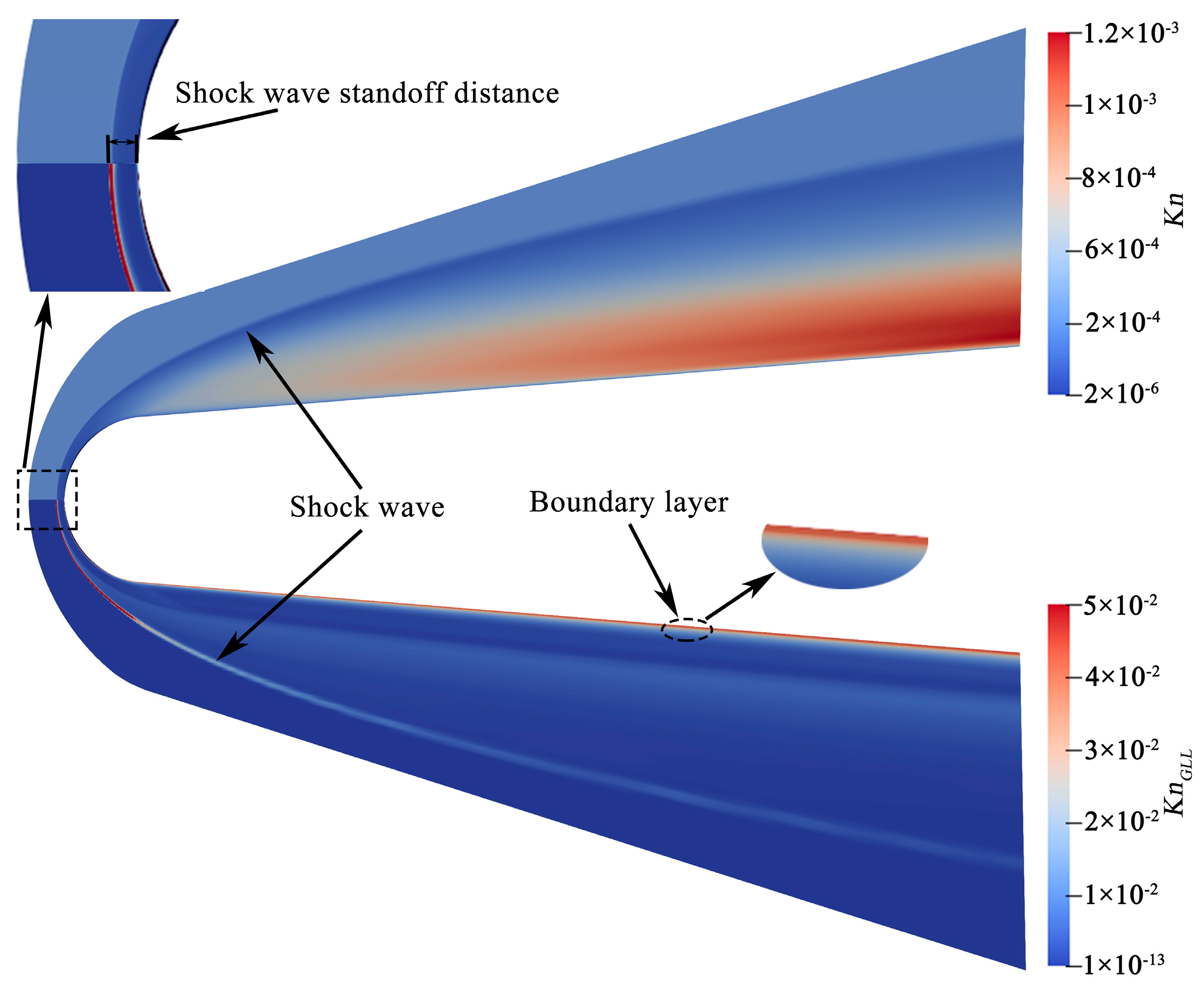
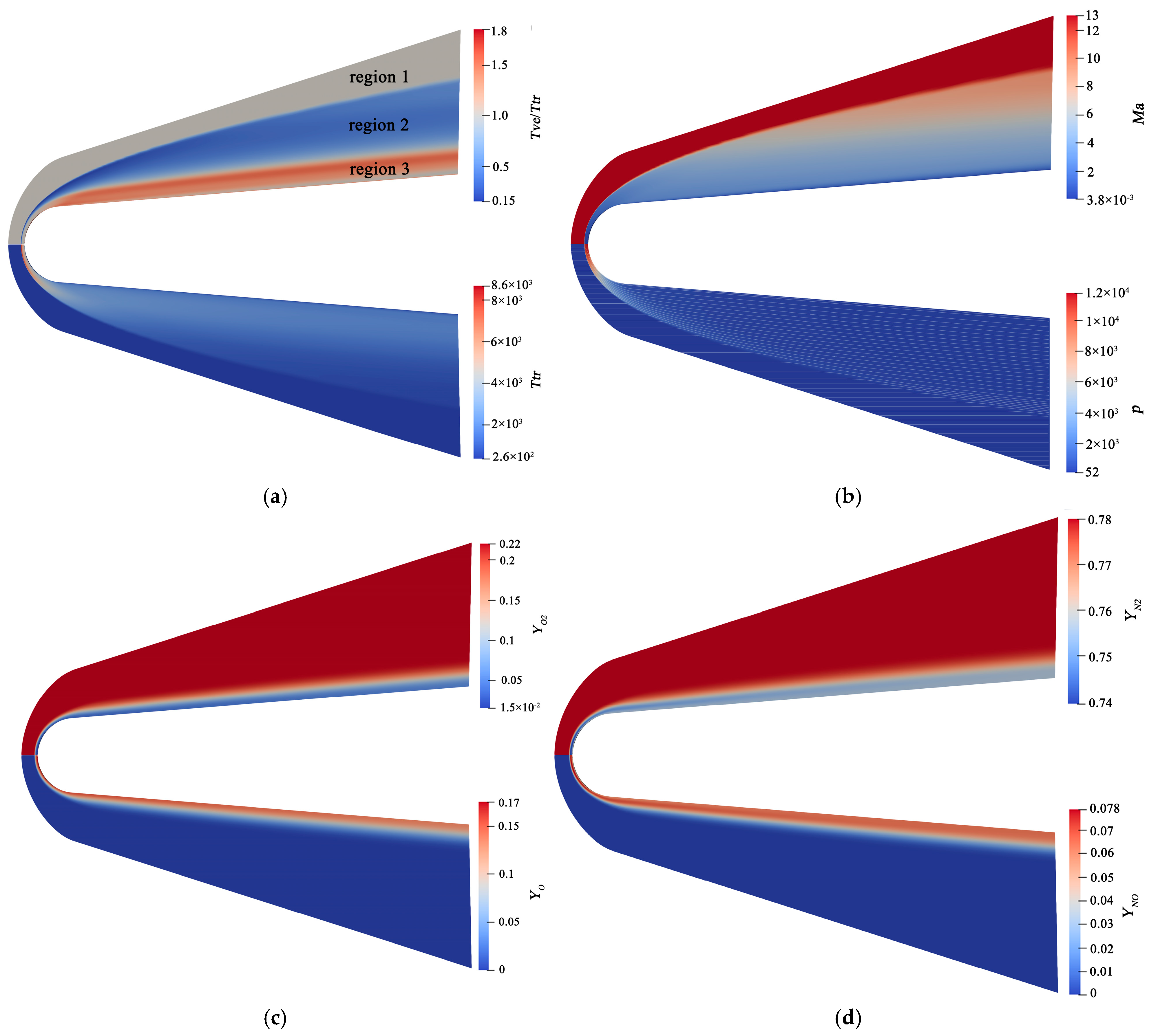
In the flight experiments of ELECTRE [7], the wall heat flux is obtained by installing ten thermocouples in the vehicle, and the measurement error of each thermocouple is given in detail. In this validation, the T_tr^0.7T_ve^0.3_Park_slip/fully catalytic and T_tr^0.7T_ve^0.3_Park_slip/non-catalytic models are employed. Figure 3 illustrates the comparison of heat flux obtained from the predictions and experiments. It can be seen that the heat flux predicted by the non-catalytic model is closer to the experimental value at the stagnation point, indicating that the catalytic efficiency is very low when the wall temperature is 343 K. In addition, most of the experimental values of the wall heat flux are in the range of predictions under the fully-catalytic wall and non-catalytic wall conditions, indicating that the solver can provide reliable predictions for the aerodynamic heat.

4.2. Flow Features

The Kn and local gradient-length Knudsen number (Kn_GLL) are usually used to express the rarefaction of gas. It is suggested that the conventional N-S equations for equilibrium flow are applied for Kn < 0.001 [21]. The local nonequilibrium regions, such as the shock wave and boundary layer, can be more accurately evaluated by Kn_GLL proposed by Boyd [44] and Wang [45], because the relaxation processes of gas properties are considered.

Figure 4 illustrates the Kn and Kn_GLL around ELECTRE simulated by the T_tr^0.7T_ve^0.3_Park_slip/non-catalytic model. From the value of Kn, it can be observed that the shock wave is closest to the surface over the stagnation point line or axis, and gradually away from the surface as it swims downstream. Therefore, the gas between the shock wave and the wall is increasingly rarefied as the shock wave moves downstream, and the rarefaction degree is the highest at the wake. Compared to Kn, which mainly describes the change in density, Kn_GLL focuses on the variation in the gradient for gas properties. As shown in Kn_GLL, the value of the gas at the regions of shock wave and boundary layer are substantially larger than that of elsewhere due to the large gradient. Moreover, the shock wave in the head region is larger than 0.05, indicating a significant nonequilibrium phenomenon in this region.

Figure 5a–d present the flow features around the ELECTRE simulated by the T_tr^0.7T_ve^0.3_Park_slip/non-catalytic model, including T_tr and the ratio of T_ve to T_tr (T_ve/T_tr), Mach number (Ma) and pressure (P), mass fractions of O₂ (Y_O2) and O (Y_O), and mass fractions of N₂ (Y_N2) and N (Y_N).

As illustrated in Figure 5a, the T_tr of flow field increases sharply behind the shock wave, and reaches 8600 K at the stagnation point, which is in good agreement with the predictions in references [7,18]. The ionization reactions usually occur with T_tr more than 8000K [9]; thus, the 5-species without ionization reactions is appropriate for this freestream. In the T_ve/T_tr contours, it can be clearly observed that three regions exist in the flow field. That is, region 1, in front of the shock wave, where the T_ve/T_tr is equal to unity; region 2, between the shock wave and boundary layer, where the T_ve/T_tr is less than unity; and region 3, around the boundary layer, where the T_ve/T_tr is larger than unity. This indicates that the thermal nonequilibrium phenomenon occurs in the region behind the shock wave. The main reason is that the relaxation time of vibrational energy mode is substantially longer than the translation time [46]. Thus, in the processes of temperature rising behind the shock wave and temperature reducing near the surfaces, the change of T_ve lags behind that of the T_tr.

In Figure 5b, the Mach number decreases significantly, and the pressure increases sharply with the air passing through the shock wave. At the stagnation point, the pressure is up to roughly 12,000 Pa. As the downstream shock wave moves away from the surface, the pressure gradually decreases and the corresponding density decreases. Thus, a rarefied gas appears in the wake region, which is indicated by the Kn contours (Figure 4).

In Figure 5c,d, due to the O₂ dissociation and the exchange reaction for generating NO at a low excitation temperature, most of O₂ are dissociated to form O, while a small part of O₂ reacts with N₂ to form NO in the head of the ELECTRE. Moreover, the new generated O and NO flow downstream along the surface. A small amount of nitrogen molecules is dissociated to produce nitrogen atoms in the head of the ELECTRE due to a high excitation temperature. The maximum value of mass fraction for N is only 0.0052, which is not presented in the related contours in this paper.

4.3. Aerodynamic Performances

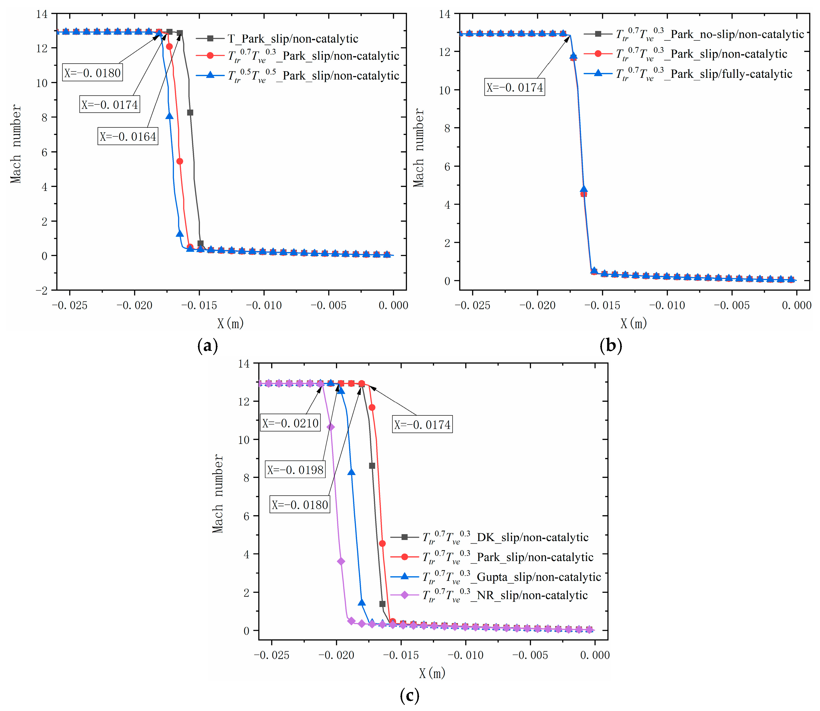
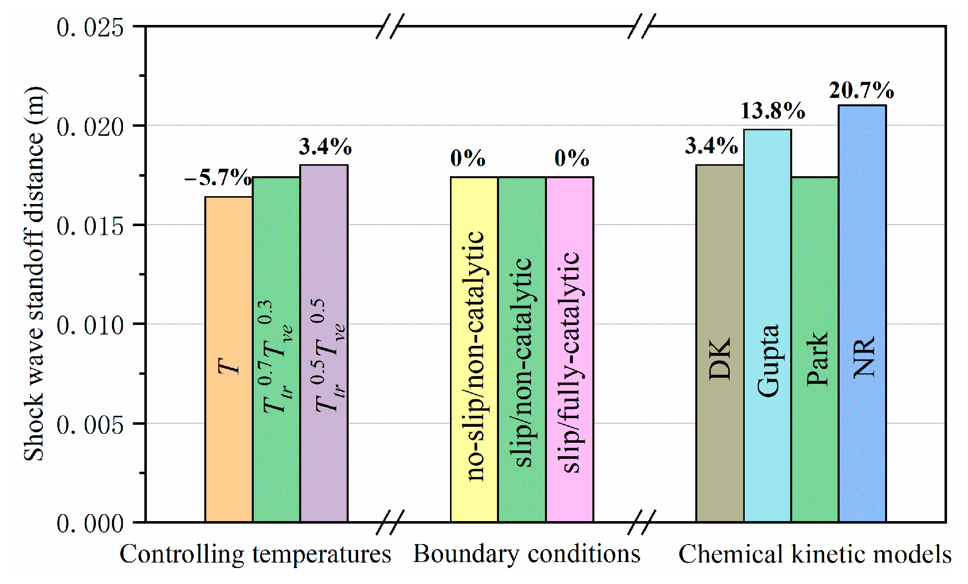
4.3.1. Shock Wave Standoff Distance

The SSD is an important property in the hypersonic flow, which can clearly indicate the characteristics of the flow structures and high temperature effects [47]. It is well-known that, at the shock wave, the velocity decreases sharply, while the temperature, density, and pressure increase dramatically. Thus, the SSD can be defined as the distance between the Mach number mutation points on the axis and the surface.

Figure 6a–c illustrate the Mach numbers along the axis of different controlling temperatures (T, T_tr^0.7T_ve^0.3 and T_tr^0.5T_ve^0.5), wall conditions (no-slip/non-catalytic, slip/non-catalytic and slip/fully-catalytic) and chemical kinetic models (DK, Gupta, Park and NR), respectively. According to the X coordinates of mutation point in Figure 6, the SSDs for different numerical models and the corresponding deviations from that of the T_tr^0.7T_ve^0.3_Park_slip/non-catalytic model are calculated, as illustrated in Figure 7. It can be observed that, compared with the SSD calculated by the T_tr^0.7T_ve^0.3_Park_slip/non-catalytic model, the SSD of the thermal equilibrium assumption (T_Park_slip/non-catalytic) decreases by 5.7%, whereas the SSD of the T_tr^0.5T_ve^0.5_Park_slip/non-catalytic model increases by 3.4%. This indicates that the SSD rises as the proportion of T_ve in the controlling temperature increases.

By comparing SSDs under three wall conditions, it is found that both catalytic and slip walls have no effect on the SSD. Evidently, the SSD is affected by different chemical kinetic models. The SSD calculated by the NR model is larger than that obtained from the models considering chemical reactions, and the deviation is up to 20.7%. In the DK, Gupta, and Park chemical kinetic models, the SSD predicted by the Gupta model is the largest, and the deviation from the result of the Park model reaches 13.8%. The SSD predicted by the DK model is approximately consistent with that of Park model.

4.3.2. Heat Flux

Figure 8a–c shows the heat flux on the surface predicted by different numerical models. It can be seen that the heat flux is more sensitive to the controlling temperature, the wall boundary condition, and the chemical kinetic model than the SSD. As shown in Figure 8a, the heat flux obtained by the T_Park_slip/non-catalytic model is larger than that calculated by the T_tr^0.7T_ve^0.3_Park_slip/non-catalytic model. Moreover, through comparing the heat flux obtained by the models of T_Park_slip/non-catalytic, T_tr^0.7T_ve^0.3_Park_slip/non-catalytic and T_tr^0.5T_ve^0.5_Park_slip/non-catalytic, it can be observed that the heat flux on the surface decreases with the proportion of T_ve in the controlling temperature increases.

As illustrated in Figure 8b, the heat flux under no-slip/non-catalytic conditions is basically consistent with that under slip/non-catalytic conditions, which reveals that the slip wall conditions have little effect on the heat flux. However, the heat flux of slip/fully-catalytic condition is significantly larger than that of two other conditions, which indicates that a large heat flux is obtained under the fully-catalytic wall.

Figure 8c depicts the heat flux of different chemical kinetic models. Apparently, the heat flux of the NR model is higher than that of the models considering chemical reactions because part of the aerodynamic heating is used for dissociation and exchange reactions. The heat flux calculated by the DK and Gupta models are in good agreement with that reported in references [7,9], respectively. Moreover, the heat flux distributions for the DK and Gupta models are almost consistent. However, the heat flux predicted by the Park model is lower than that calculated by the DK and Gupta models.

Figure 9 illustrates the heat flux and deviations for different numerical models from that based on the T_tr^0.7T_ve^0.3_Park_slip/non-catalytic model at stagnation point. It can be observed that the heat flux predicted by the fully catalytic model is the largest, which is 62.2% higher than that calculated by the non-catalytic model. Moreover, the prediction of stagnation point heat flux increases by 29.0% without considering the chemical reactions and rises by 15.3% under the thermal nonequilibrium assumption. Compared with the results of the DK and Gupta models, the heat flux predicted by the Park model is lower, and the absolute deviation is up to 9.8%.

4.4. Discussion the Influence of Numerical Models on the Heat Flux

As found above, the heat flux is more sensitive than SSD to the numerical models. The heat fluxes on the surface of the 1T and 2T models are defined as

$$\begin{array}{l}{q}_w=q_{w,con}+q_{w,diff}=({\kappa }_{tr}{\displaystyle \frac{\partial T}{\partial n}}+{\kappa }_{ve}{\displaystyle \frac{\partial T}{\partial n}})+\rho {\displaystyle \sum _s{D}_s{h}_s\frac{\partial Y_s}{\partial n}}\mathrm{for}1\mathrm{T}\mathrm{model}\\ q_w=q_{w,con}+q_{w,diff}=({\kappa }_{tr}{\displaystyle \frac{\partial T_{tr}}{\partial n}}+{\kappa }_{ve}{\displaystyle \frac{\partial T_{ve}}{\partial n}})+\rho {\displaystyle \sum _s{D}_s{h}_s\frac{\partial Y_s}{\partial n}}\mathrm{for}2\mathrm{T}\mathrm{model}\end{array}$$

(22)

where q_w,con is the convective heat flux, q_w,diff is the diffusion heat flux, κ_tr(∂T/∂n) and κ_tr(∂T_tr/∂n) represent the trans-rotational convective heat fluxes, κ_ve(∂T/∂n) and κ_ve(∂T_tr/∂n) represent the vibro-electronic convective heat fluxes.

As presented in Figure 9, the prediction of heat flux based on the T_Park_slip/non-catalytic model is 15.3% larger than that on the T_tr^0.7T_ve^0.3_Park_slip/non-catalytic model. There are two possible reasons for this result, one is the different degree of chemical reactions, and the other is the thermal equilibrium/nonequilibrium assumption. In order to eliminate the influence of chemical reactions, the heat fluxes of the 1T and 2T models without chemical reactions are investigated, as seen in Figure 10. As shown, the stagnation point heat flux of the 1T model is 30% bigger than that of the 2T model. This prediction deviation (30%) is bigger than that of considering reactions (15.3%), revealing that the thermal equilibrium/nonequilibrium assumption is primary reason for the prediction deviation of heat flux.

Regardless of the catalytic wall, the heat flux can be considered to be composed of trans-rotational and vibro-electronic convective heat fluxes. As shown in Figure 11, the trans-rotational convective heat flux of the 1T model is apparently larger than that of the 2T models, whereas the vibro-rotational convective heat flux of 1T model is smaller than that of the 2T model. The fundamental reason is that the relaxation processes of trans-rotational and vibro-electronic energies [48] is considered in the 2T model. Near the surface, T_tr is lower than T_ve in the 2T model, while T_tr is equal to T_ve in the 1T model. However, the vibro-electronic convective heat flux accounts for a negligible proportion of the total heat flux.

The heat flux predicted by a fully catalytic wall is 62.2% larger than by non-catalytic wall. This is because the diffusive heat flux will be generated under the catalytic wall, but it does not exist under the non-catalytic wall. The details of the convective, diffusive, and total heat fluxes with the fully catalytic wall condition are presented in Figure 12. It can be observed that the diffusive heat flux accounts for a considerable proportion of the total heat flux. Here, the fully catalytic wall is an extreme case with a fully recombination reaction. In fact, the catalytic state of the surface is between the non-catalytic and fully catalytic conditions, namely, finite-rate catalytic [49]. However, an appropriate catalytic recombination coefficient related to the surface materials and temperature is required in the finite-rate model [28,50]. Thus, the actual values of heat flux range between the values of the non-catalytic and fully catalytic walls, in theory.

Besides the NR model, the heat flux predicted by Gupta is much larger than that by the DK and Park model. This is mainly due to the different reaction rates for various chemical kinetic models. Figure 13 shows the forward rate coefficients of O₂ and N₂ dissociations for the Gupta, Park, and DK models. As shown, the forward rate coefficients of the Gupta model are apparently lower than those of the DK and Park models, which indicates the dissociation level of O₂ and N₂ molecules for the Gupta model is lower than the DK and Park models. This means the absorbed heat from the flow field due to chemical reactions of the Gupta model is lower than that of the DK and Park models. Thus, the heat flux predicted by the Gupta model is the largest.

5. Conclusions

In this paper, the influences of various types of numerical models on the aerodynamic performances (SSD and heat flux) of ELECTRE at 293 sec and 53.3 km with velocity of 4230 m/s are investigated. Several types of numerical models include the thermal equilibrium/nonequilibrium (1T/2T), controlling temperatures (T_tr^0.7T_ve^0.3, T_tr^0.5T_ve^0.5), surface boundary conditions (no slip/non-catalytic, slip/non-catalytic, and slip/fully catalytic) and chemical kinetic models (DK, Park, Gupta, and NR). The main conclusions are drawn as follows:

(1) The flow features around the ELECTRE vehicle are investigated. It is found that an obvious thermal nonequilibrium occurs behind the shock wave in which the change in the T_ve lags behind the variation in the T_tr. Apparent chemical reactions exist in the head of the ELECTRE, most of the O₂ is dissociated to form O, while a small part of the O₂ reacts with N₂ to form NO.

(2) The chemical kinetic model is the most significant reason for influencing the value of SSD. Without considering the chemical reactions, the SSD is the largest, and deviation from that obtained by the Park model is up to 20.7%. The comparisons of SSDs calculated by the Gupta, DK, and Park models show that the SSD gradually decreases with the increase in chemical reaction rate. The SSD is also affected by the thermal equilibrium/nonequilibrium assumption and the controlling temperature. The higher the proportion of T_ve in the controlling temperature is, the larger the SSD is.

(3) The surface catalytic condition is a critical factor in the prediction of heat flux, the stagnation point heat flux calculated by the fully catalytic wall is 62.2% higher than that by the non-catalytic wall. The heat flux is influenced by the chemical reaction rate. As the chemical reaction rate increases, the heat flux calculated by the NR, Gupta, DK, and Park models decreases in turn. The heat flux is also affected by the thermal equilibrium/nonequilibrium assumption and the controlling temperature to a certain extent. Because the international energies relaxation process is considered in the 2T model, the trans-rotational convective heat flux of the 2T model is much lower than that of the 1T model, which results in the heat flux predicted by the 2T model being lower than that predicted by the 1T model. In addition, the heat flux decreases with an increase in the proportion of T_ve in the controlling temperature.

This paper systematically evaluated several numerical models on the heat flux and the SSD in hypersonic nonequilibrium flows and explained why these numerical models affect the aerodynamic heating, which can provide effective reference for the accurate prediction of the aerodynamic heating of hypersonic vehicles.

References

1. Longo, J.M.A.; Hannemann, K.; Hannemann, V. The challenge of modeling high speed flows. In Proceedings of the EUROSIM 2007, Ljubljana, Slovenia, 9–13 September 2007. [Google Scholar]
2. Schwartzentruber, T.E.; Boyd, I.D. Progress and future prospects for particle-based simulation of hypersonic flow. Prog. Aerosp. Sci. 2015, 72, 66–79. [Google Scholar] [CrossRef]
3. Karpenko, M.; Stosiak, M.; Šukevičius, Š.; Skačkauskas, P.; Urbanowicz, K.; Deptuła, A. Hydrodynamic Processes in Angular Fitting Connections of a Transport Machine’s Hydraulic Drive. Machines 2023, 11, 355. [Google Scholar] [CrossRef]
4. Lee, J.H. Basic governing equations for the flight regimes of aeroassisted orbital transfer vehicles. In Proceedings of the AlAA 19th Thermophysics Conference, Snowmass, CO, USA, 25–28 June 1984. [Google Scholar]
5. Park, C. Assessment of two-temperature kinetic model for ionizing air. J. Thermophys. Heat Transf. 1989, 3, 233–244. [Google Scholar] [CrossRef]
6. Zhang, W.; Zhang, Z.; Wang, X.; Su, T. A review of the mathematical modeling of equilibrium and nonequilibrium hypersonic flows. Adv. Aerodyn. 2022, 4, 38. [Google Scholar] [CrossRef]
7. Muylaert, J.; Walpot, L.; Haeuser, J.; Sagnier, P.; Devezeaux, D.; Papirnyk, O.; Lourme, D. Standard model testing in the European High Enthalpy Facility F4 andextrapolation to flight. In Proceedings of the AIAA 17th Aerospace Ground Testing Conference, Nashville, TN, USA, 6–8 July 1992. [Google Scholar]
8. Hao, J.; Wang, J.; Lee, C. Numerical study of hypersonic flows over reentry configurations with different chemical nonequilibrium models. Acta Astronaut. 2016, 126, 1–10. [Google Scholar] [CrossRef]
9. Niu, Q.; Yuan, Z.; Dong, S.; Tan, H. Assessment of nonequilibrium air-chemistry models on species formation in hypersonic shock layer. Int. J. Heat Mass Transf. 2018, 127, 703–716. [Google Scholar] [CrossRef]
10. Kim, J.G.; Kang, S.H.; Park, S.H. Thermochemical nonequilibrium modeling of oxygen in hypersonic air flows. Int. J. Heat Mass Transf. 2020, 148, 119059. [Google Scholar] [CrossRef]
11. Harvey, J.K.; Holden, M.S.; Wadhams, T.P. Code validation study of laminar shock/boundary layer and shock/shock interactions in hypersonic flow Part B: Comparison with Navier-Stokes and DSMC Solutions. In Proceedings of the 39th Aerospace Sciences Meeting and Exhibit, Reno, NV, USA, 8–11 January 2001. [Google Scholar]
12. MacLean, M.; Holden, M.A. Dufrene, Comparison Between CFD and Measurements for Real-Gas Effects on Laminar Shock Wave Boundary Layer Interaction. In Proceedings of the AIAA Aviation 44th AIAA Fluid Dynamics Conference, Atlanta, GA, USA, 16–20 June 2014. [Google Scholar]
13. Holden, M.; Wadhams, T.; Harvey, J.; Candler, G. Comparisons between Dsmc and Navier-Stokes Solutions and Measurements in Regions of Laiviinar Shock Wave Boundary Layer Interaction in Hypersonic Flows, NATO RTO-TR-AVT-007-V3. In Proceedings of the 40th AIAA Aerospace Sciences Meeting & Exhibit, Reno, NV, USA, 9–12 January 2006. [Google Scholar]
14. Candler, G.V.; Nompelis, I.; Druguet, M.-C.; Holden, M.S.; Wadhams, T.P.; CUBRC, B.N.; Boyd, I.D.; Wang, W.-L. CFD Validation for Hypersonic Flight: Hypersonic Double-Cone Flow Simulations. In Proceedings of the 40th AIAA Aerospace Sciences Meeting and Exhibit, Reno, NV, USA, 14–17 January 2002. [Google Scholar]
15. Nompelis, I.; Candler, G.V.; Holden, M.S. Effect of Vibrational Nonequilibrium on Hypersonic Double-Cone Experiments. AIAA J. 2003, 41, 2162–2169. [Google Scholar] [CrossRef]
16. Hao, J.; Wang, J.; Lee, C. Numerical Simulation of High-Enthalpy Double-Cone Flows. AIAA J. 2017, 55, 2471–2475. [Google Scholar] [CrossRef]
17. Kianvashrad, N.; Knight, D. Simulation of Hypersonic Shock-Wave–Laminar-Boundary-Layer Interaction on Hollow Cylinder Flare. AIAA J. 2017, 55, 322–326. [Google Scholar] [CrossRef]
18. Wang, X.Y.; Yan, C.; Zheng, Y.K.; Li, E.L. Assessment of chemical kinetic models on hypersonic flow heat transfer. Int. J. Heat Mass Transf. 2017, 111, 356–366. [Google Scholar] [CrossRef]
19. Holloway, M.E.; Hanquist, K.M.; Boyd, I.D. Effect of Thermochemistry Modeling on Hypersonic Flow Over a Double Cone. In Proceedings of the AIAA SciTech Forum, San Diego, CA, USA, 7–11 January 2019. [Google Scholar]
20. Dobrov, Y.; Gimadiev, V.; Karpenko, A.; Volkov, K. Numerical simulation of hypersonic flow with non-equilibrium chemical reactions around sphere. Acta Astronaut. 2022, 194, 468–479. [Google Scholar] [CrossRef]
21. Schouler, M.; Prévereaud, Y.; Mieussens, L. Survey of flight and numerical data of hypersonic rarefied flows encountered in earth orbit and atmospheric reentry. Prog. Aerosp. Sci. 2020, 118, 100638. [Google Scholar] [CrossRef]
22. Lofthouse, A.J.; Scalabrin, L.C.; Boyd, I.D. Velocity Slip and Temperature Jump in Hypersonic Aerothermodynamics. J. Thermophys. Heat Transf. 2008, 22, 38–49. [Google Scholar] [CrossRef]
23. Massuti-Ballester, B.; Pidan, S.; Herdrich, G.; Fertig, M. Recent catalysis measurements at IRS. Adv. Space Res. 2015, 56, 742–765. [Google Scholar] [CrossRef]
24. MacLean, M.; Holden, M. Catalytic Effects on Heat Transfer Measurements for Aerothermal Studies with CO2. In Proceedings of the 44th AIAA Aerospace Sciences Meeting and Exhibit, Reno, NV, USA, 9–12 January 2006. [Google Scholar]
25. Viviani, A.; Pezzella, G. Catalytic Effects on Non-Equilibrium Aerothermodynamics of a Reentry Vehicle. In Proceedings of the 45th AIAA Aerospace Sciences Meeting and Exhibit, Reno, NV, USA, 8–11 January 2007. [Google Scholar]
26. Yang, J.; Liu, M. Numerical analysis of hypersonic thermochemical non-equilibrium environment for an entry configuration in ionized flow. Chin. J. Aeronaut. 2019, 32, 2641–2654. [Google Scholar] [CrossRef]
27. Needels, J.T.; Duzel, U.; Hanquist, K.M.; Alonso, J.J. Sensitivity Analysis of Gas-Surface Modeling in Nonequilibrium Flows. In Proceedings of the AIAA SciTech Forum, San Diego, CA, USA, 3–7 January 2022. [Google Scholar]
28. Yang, Y.; Sethuraman, V.R.P.; Kim, H.; Kim, J.G. Determination of surface catalysis on copper oxide in a shock tube using thermochemical nonequilibrium CFD analysis. Acta Astronaut. 2022, 193, 75–89. [Google Scholar] [CrossRef]
29. Bechina, A.I.; Kustova, E.V. Rotational Energy Relaxation Time for Vibrationally Excited Molecules, Vestnik St. Petersburg University. Mathematics 2019, 52, 117–129. [Google Scholar]
30. Casseau, V.; Scanlon, T.J.; John, B.; Emerson, D.R.; Brown, R.E. Hypersonic simulations using open-source CFD and DSMC solvers. AIP Conf. Proc. 1786, 050006. [Google Scholar] [CrossRef]
31. Casseau, V. An Open-Source CFD Solver for Planetary Entry; University of Strathclyde: Glasgow, UK, 2017. [Google Scholar]
32. Candler, G.V.; Nompelis, I. Computational Fluid Dynamics for Atmospheric Entry, NATO RTO-EN-AVT-162. 2009. Available online: https://docslib.org/doc/13466456/computational-fluid-dynamics-for-atmospheric-entry (accessed on 19 November 2024).
33. Alkandry, H.; Boyd, I.; Martin, A. Comparison of Models for Mixture Transport Properties for Numerical Simulations of Ablative Heat-Shields. In Proceedings of the 51st AIAA Aerospace Sciences Meeting including the New Horizons Forum and Aerospace Exposition, Grapevine, TX, USA, 7–10 January 2013. [Google Scholar]
34. Park, C. Nonequilibrium Hypersonic Aerothermodynamics; Wiley International: New York, NY, USA, 1990. [Google Scholar]
35. Blottner, F.G.; Johnson, M.; Ellis, M. Chemically Reacting Viscous Flow Program for Multicomponent Gas Mixture; Report no. SC-RR-70-754; Sandia National Lab. (SNL-NM): Albuquerque, NM, USA, 1971. [Google Scholar]
36. Armaly, B.F.; Rolla, M.; Sutton, K. Viscosity of Multicomponent Partially Ionized Gas Mixtures. In Proceedings of the AlAA 15th thermophysics conference, Snowmass, CO, USA, 14–16 July 1980. [Google Scholar]
37. Greenshields, C.J.; Reese, J.M. Rarefied hypersonic flow simulations using the Navier–Stokes equations with non-equilibrium boundary conditions. Prog. Aerosp. Sci. 2012, 52, 80–87. [Google Scholar] [CrossRef]
38. Maxwell, J.C. On Stresses in Rarified Gases Arising from Inequalities of Temperature. Philos. Trans. R. Soc. Lond. 1879, 170, 231–256. [Google Scholar]
39. Yuan, Z.; Huang, S.; Gao, X.; Liu, J. Effects of Surface-Catalysis Efficiency on Aeroheating Characteristics in Hypersonic Flow. J. Aerosp. Eng. 2016, 30, 04016086. [Google Scholar] [CrossRef]
40. Dunn, M.G.; Kang, S. Theoretical and Experimental Studies of Reentry Plasmas; NASA CR-2232; NASA: Washington, DC, USA, 1973. [Google Scholar]
41. Gupta, R.N.; Yos, J.M.; Thompson, R.A. A review of reaction rates and thermodynamic and transport properties for the 11-species air model for chemical and thermal nonequilibrium calculations to 30000 K, NASA RP-1232 1990, 1–86. Available online: https://ntrs.nasa.gov/api/citations/19900017748/downloads/19900017748.pdf (accessed on 19 November 2024).
42. Park, C. Review of Chemical-Kinetic Problems of Future NASA Missions, I: Earth Entries. J. Thermophys Heat Transf. 1993, 7, 385–398. [Google Scholar] [CrossRef]
43. Qu, F.; Chen, J.; Sun, D.; Bai, J.; Zuo, G. A grid strategy for predicting the space plane’s hypersonic aerodynamic heating loads. Aerosp. Sci. Technol. 2019, 86, 659–670. [Google Scholar] [CrossRef]
44. Boyd, I.D.; Chen, G.; Candler, G.V. Predicting failure of the continuum fluid equations in transitional hypersonic flows. Phys. Fluids 1995, 7, 210–219. [Google Scholar] [CrossRef]
45. Wang, W.-L.; Boyd, I.D. Predicting continuum breakdown in hypersonic viscous flows. Phys. Fluids 2003, 15, 91–100. [Google Scholar] [CrossRef]
46. Istomin, V.A.; Oblapenko, G.P. Transport coefficients in high-temperature ionized air flows with electronic excitation. Phys. Plasmas 2018, 25, 013514. [Google Scholar] [CrossRef]
47. Hu, Y.; Huang, H.; Guo, J. Shock wave standoff distance of near space hypersonic vehicles. Sci. China Technol. Sci. 2017, 60, 1123–1131. [Google Scholar] [CrossRef]
48. Du, Y.-W.; Sun, S.-R.; Tan, M.-J.; Zhou, Y.; Chen, X.; Meng, X.; Wang, H.-X. Non-equilibrium simulation of energy relaxation for earth reentry utilizing a collisional-radiative model. Acta Astronaut. 2022, 193, 521–537. [Google Scholar] [CrossRef]
49. Yang, X.; Gui, Y.; Xiao, G.; Du, Y.; Liu, L.; Wei, D. Reacting gas-surface interaction and heat transfer characteristics for high-enthalpy and hypersonic dissociated carbon dioxide flow. Int. J. Heat Mass Transf. 2020, 146, 118869. [Google Scholar] [CrossRef]
50. Gimelshein, S.F.; Wysong, I.J. Gas-Phase Recombination Effect on Surface Heating in Nonequilibrium Hypersonic Flows. J. Thermophys. Heat Transf. 2019, 33, 638–646. [Google Scholar] [CrossRef]
Figure 1. Grid of axisymmetric model.
Processes 12 02629 g001
Figure 2. Trans-rotational temperatures along the axis for different grids.
Processes 12 02629 g002
Figure 3. Predictions and experiment data of wall heat flux.
Processes 12 02629 g003
Figure 4. Kn of ELECTRE with 2T_Park_slip/non-catalytic model.
Processes 12 02629 g004
Figure 5. Flow fields of ELECTRE with Ttr0.7Tve0.3_Park_slip/non-catalytic model, (a) Tve/Ttr and Ttr, (b) Ma and P, (c) YO2 and YO, (d) YN2 and YNO.
Processes 12 02629 g005
Figure 6. Mach numbers along axis of different numerical models, (a) different controlling temperatures, (b) different boundary conditions, (c) different chemical kinetic models.
Processes 12 02629 g006
Figure 7. Shock wave standoff distance of different numerical models.
Processes 12 02629 g007
Figure 8. Heat fluxes of different numerical models, (a) different controlling temperatures, (b) different boundary conditions, (c) different chemical kinetic models.
Processes 12 02629 g008
Figure 9. Stagnation point heat flux of different numerical models.
Processes 12 02629 g009
Figure 10. Heat flux of 1T and 2T models without reactions.
Processes 12 02629 g010
Figure 11. Trans-rotational and vibro-electronic convective heat fluxes.
Processes 12 02629 g011
Figure 12. Heat flux for fully-catalytic wall.
Processes 12 02629 g012
Figure 13. Forward rate coefficient of different chemical kinetic models.
Processes 12 02629 g013