


Generalized Conditional Feedback System with Model Uncertainty


Abstract
:1. Introduction
- (1)
- A GCF scheme is proposed to control industrial processes with model uncertainty that simultaneously guarantees closed-loop performance and robustness.
- (2)
- The effectiveness of the proposed GCF scheme is validated by case studies and a half-quadrotor system control test.
2. Problem Formulation
2.1. Model Uncertainty
2.2. Control Problem
2.3. Nominal Model
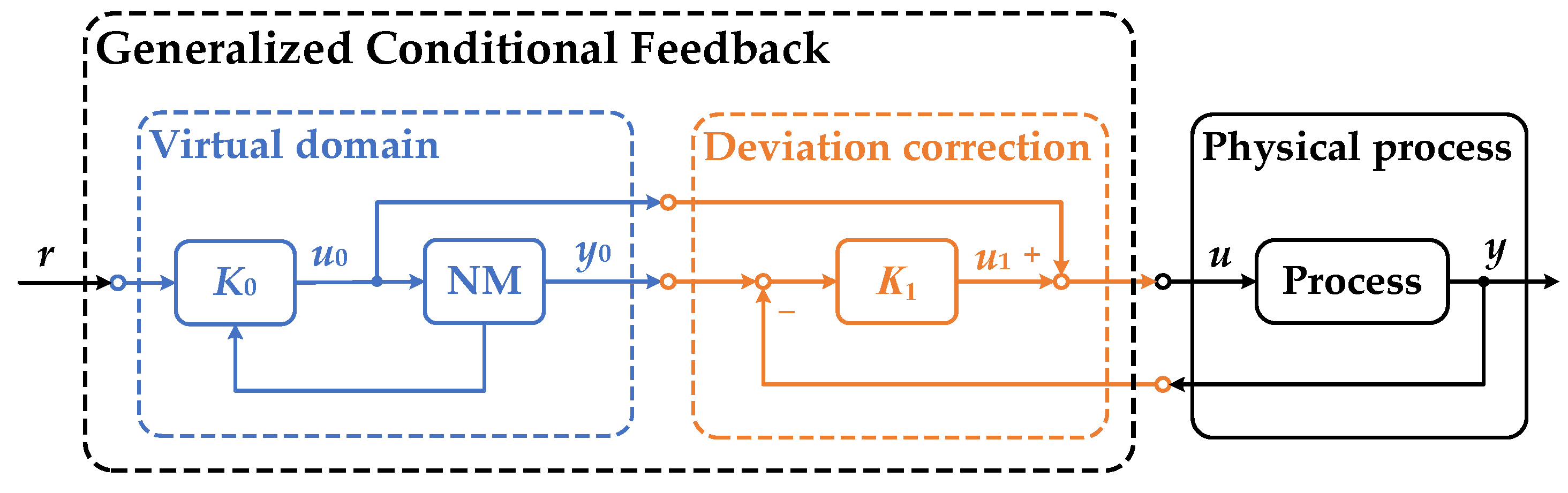
3. Generalized Conditional Feedback
3.1. Control Algorithm
- I.
- There are two systems being controlled: the NM (5) is virtual, and the controlled process (1) is physical.
- II.
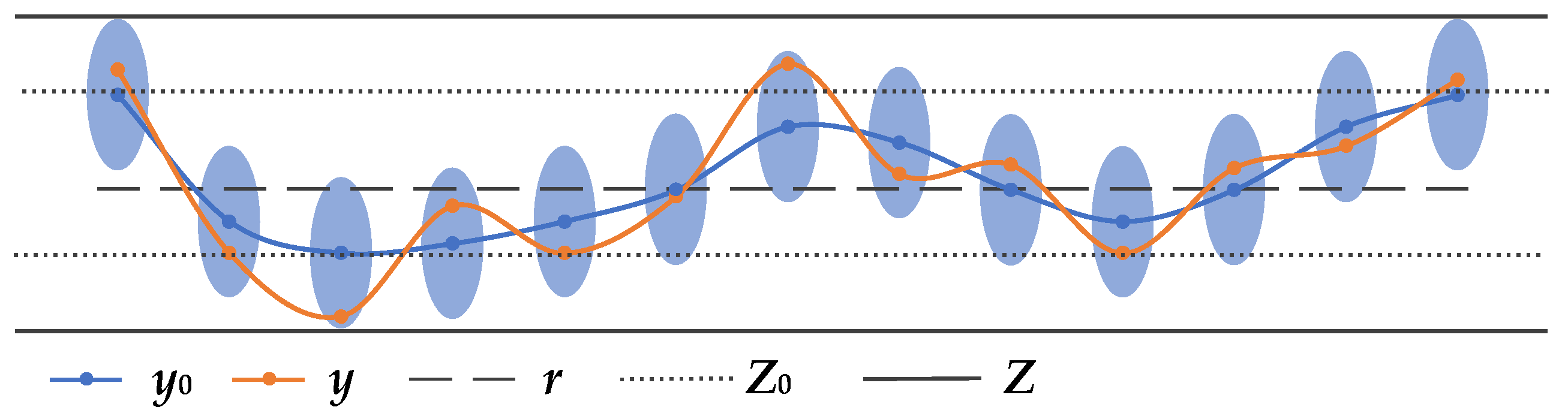
- In the virtual domain, the trajectory of the virtual NM is optimized to be the desired state of the physical process.
- III.
- The two systems are connected only by the deviation correction controller, which essentially tries to drive the physical process to track the desired trajectory coming from the virtual domain.
- I.
- The controller in the virtual domain can be any feasible control strategy that is capable of optimizing NM to a specified state.
- II.
- III.
- The stability and the optimization are unified. The controller in the virtual domain ensures optimization and the ancillary correction controller guarantees stability.
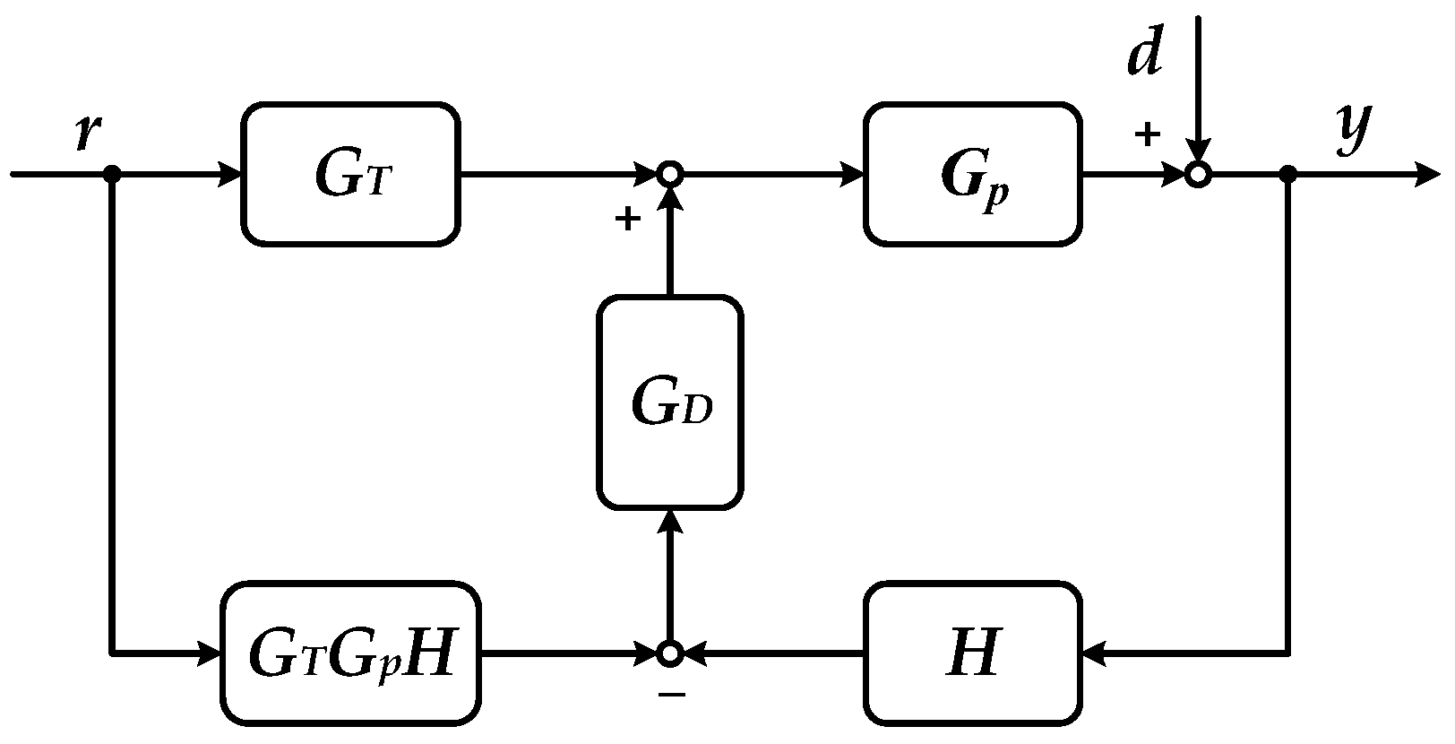
3.2. Conditional Feedback
3.3. Closed-loop Performance Robustness
3.4. Practice Procedure
| Algorithm 1: Practice procedure of the GCF scheme. |
| 1: system identification (offline) |
| get a nominal model |
| 2: simulation design (offline) |
| K0 ← Equation (6) |
| K1 ← Equation (7) |
| 3: practice (online) |
| startup control |
| u ← K1 (r, y, u) |
| u0 ← u |
| then |
| u0 ← K0 (r, y0, u0) |
| u1 ← K1 (y, y0, u0, u1) |
| u ← u0 + u1 |
4. Simulation Illustration
- I.
- State observers are designed when FSFC and LRQ are applied to uncertain models. The observer estimation speed is selected to be 3~5 times the closed-loop response.
- II.
- For processes, G1(s)~G4(s), the state-space models are all expressed as the second controllable canonical form.
- III.
- The pole placements and the cost functions are listed in Table 4.
- IV.

| Control Methods | Processes | Placed Poles | |
|---|---|---|---|
| Closed-Loop | State Observer | ||
| FSFC | G1(s) | [−1+j, −1−j, −1 −2] | [−2+2j, −2−2j, −2 −4] |
| G2(s) | [−7+5j, −7−5j, −10] | [−15+10j, −15−10j, −15] | |
| LQR | G3(s) | Cost function: | [−8+4j, −8−4j] |
| G4(s) | [−10+5j, −10−5j] | ||
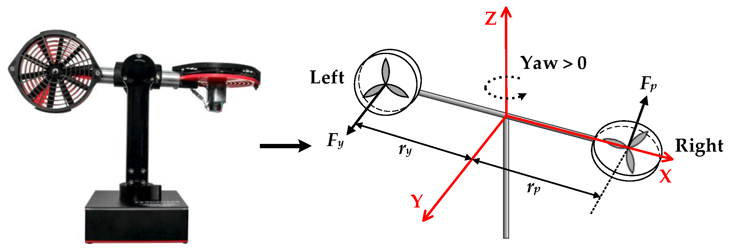
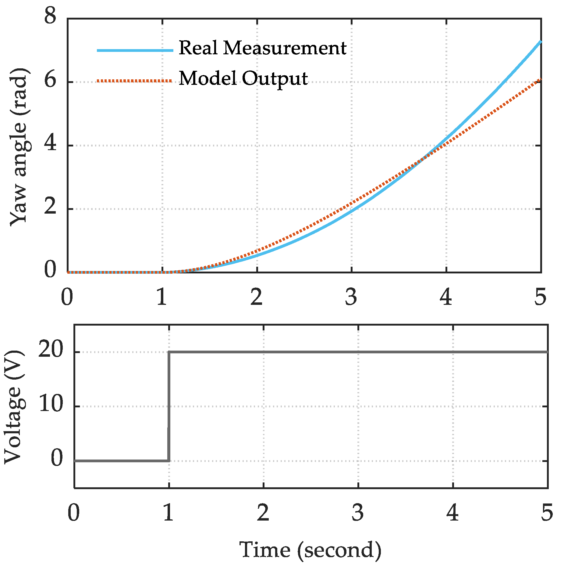
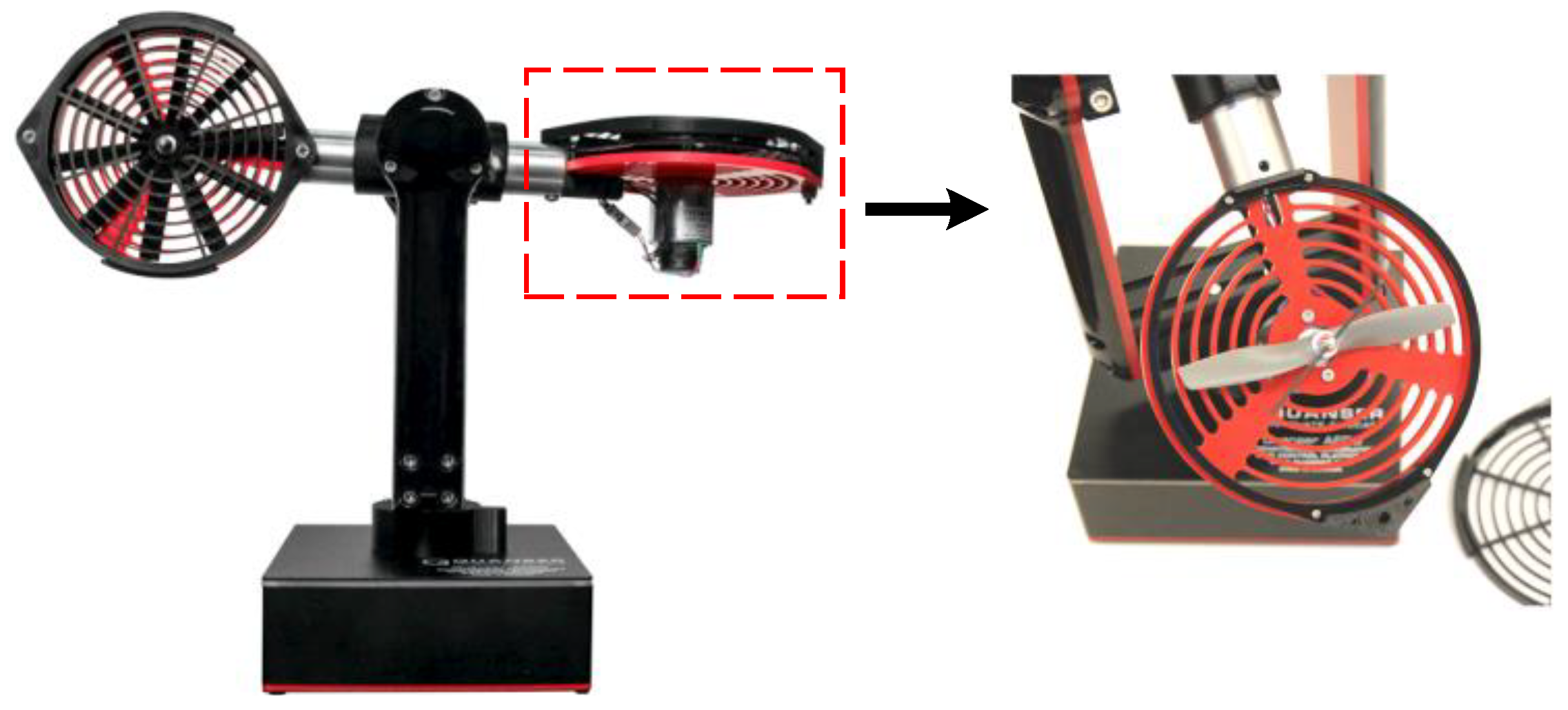
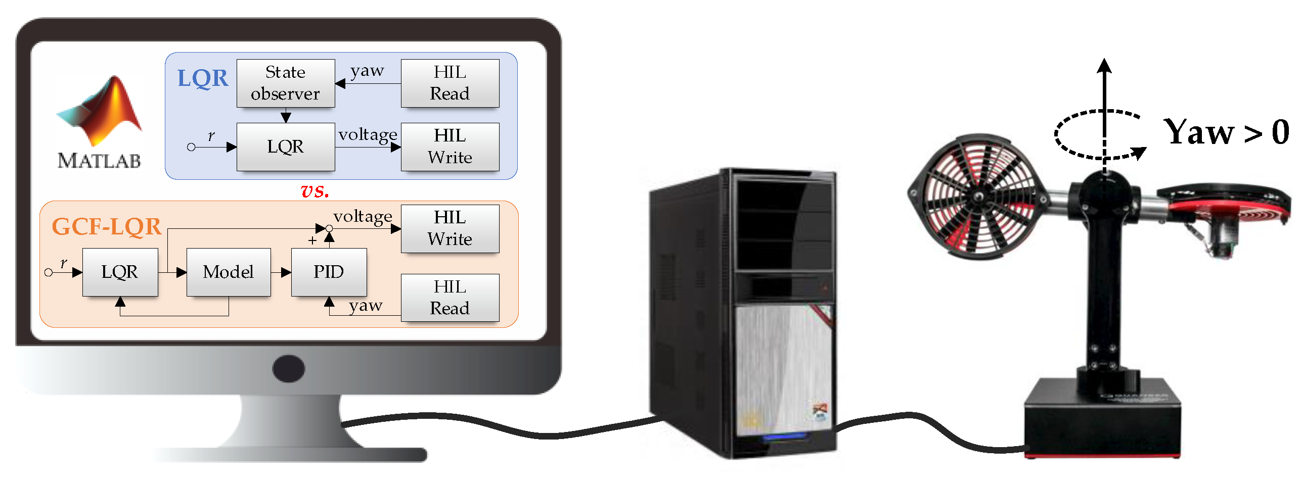
5. Experiment Validation on a Half-Quadrotor System
5.1. System Model
5.2. Control Structure
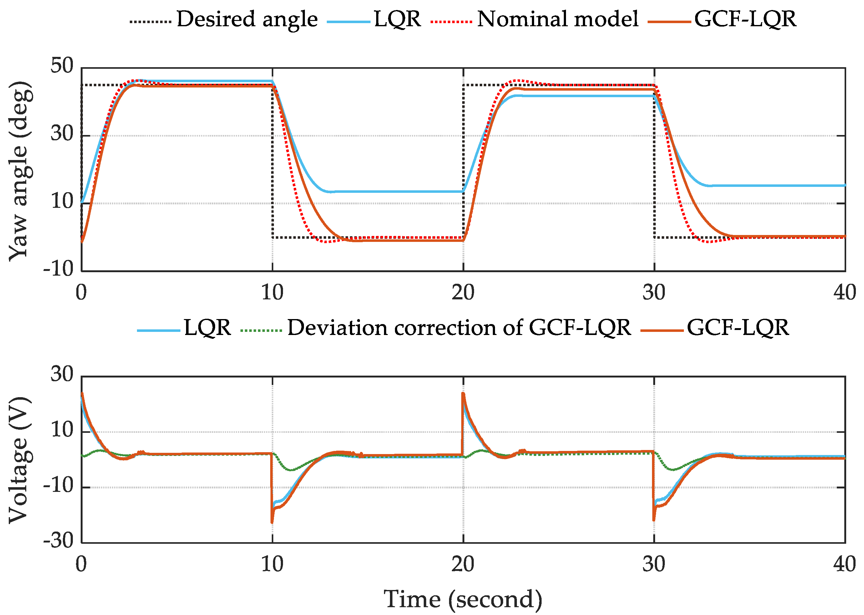
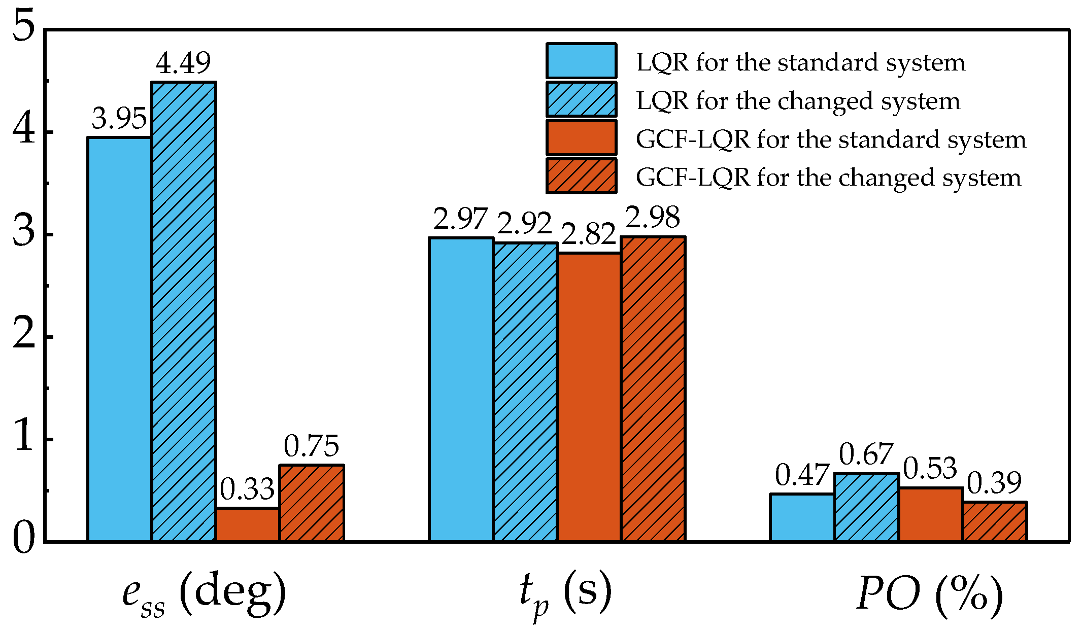
5.3. Experiment Results
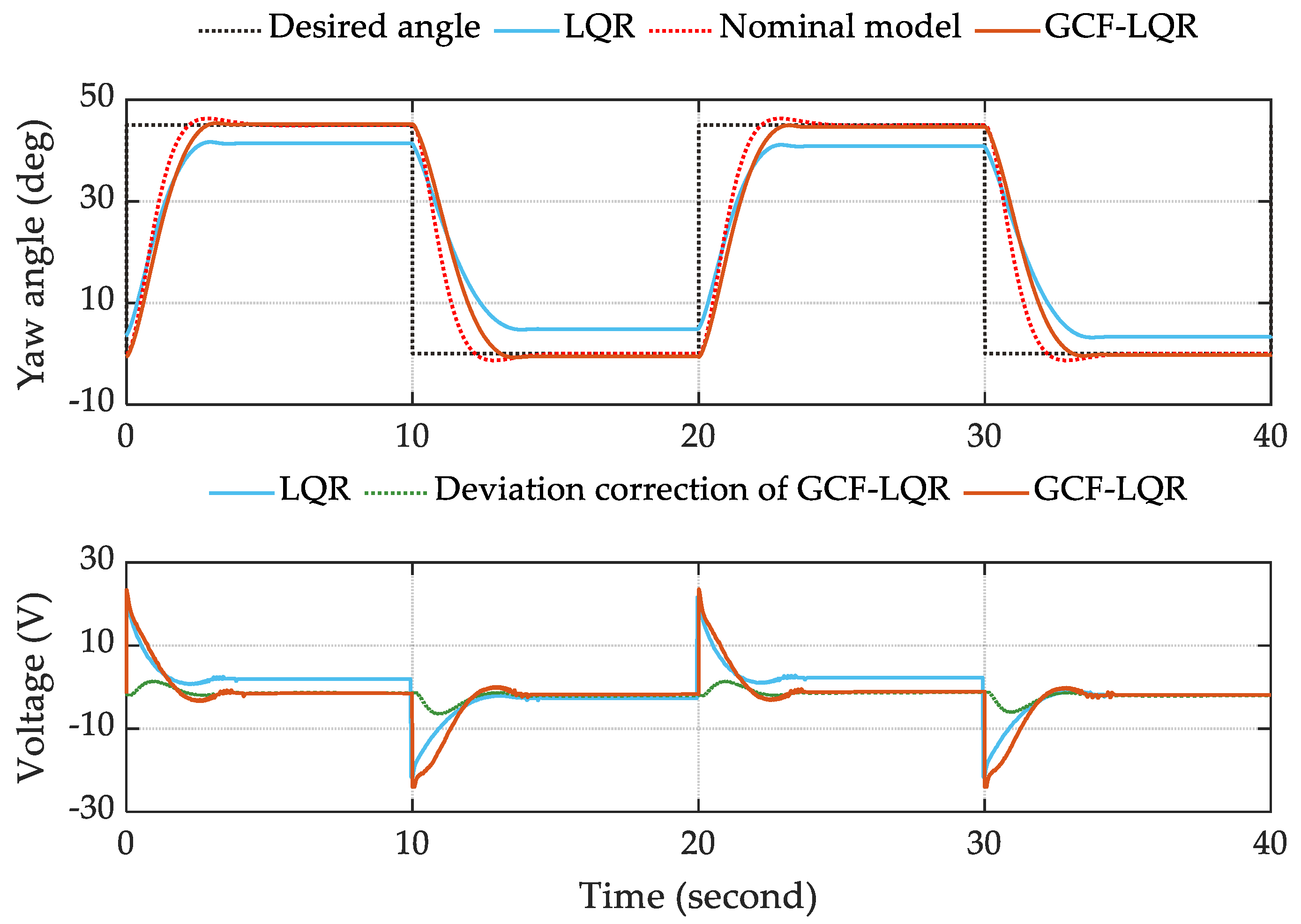
- Steady-state error: ess ≤ 2 deg.
- Peak time: tp ≤ 3 s.
- Percent Overshoot: PO ≤ 2%.
5.3.1. Experiment 1: Standard System
5.3.2. Experiment 2: Changing the Propeller
6. Conclusions
Author Contributions
Funding
Data Availability Statement
Conflicts of Interest
References
- Degrave, J.; Felici, F.; Buchli, J.; Neunert, M.; Tracey, B.; Carpanese, F.; Ewalds, T.; Hafner, R.; Abdolmaleki, A.; de las Casas, D.; et al. Magnetic control of tokamak plasmas through deep reinforcement learning. Nature 2022, 602, 414–419. [Google Scholar] [CrossRef] [PubMed]
- Tsien, H.S. Engineering Cybernetics; McGraw-Hill: New York, NY, USA, 1954. [Google Scholar]
- Samad, T.; Bauer, M.; Bortoff, S.; Di Cairano, S.; Fagiano, L.; Odgaard, P.F.; Rhinehart, R.R.; Sánchez-Peña, R.; Serbezov, A.; Ankersen, F.; et al. Industry engagement with control research: Perspective and messages. Annu. Rev. Control 2020, 49, 1–14. [Google Scholar] [CrossRef]
- Yedavalli, R.K. Robust Control of Uncertain Dynamic Systems: A Linear State Space Approach; Springer: New York, NY, USA, 2013. [Google Scholar]
- Brockett, R. New Issues in the Mathematics of Control. In Mathematics Unlimited—2001 and Beyond; Engquist, B., Schmid, W., Eds.; Springer Berlin Heidelberg: Berlin/Heidelberg, Germany, 2001; pp. 189–219. [Google Scholar]
- Petersen, I.R.; Ugrinovskii, V.A.; Savkin, A.V. Robust Control Design Using H−∞ Methods; Springer: London, UK, 2000. [Google Scholar]
- Sun, L.; Li, D.H.; Lee, K.Y. Optimal disturbance rejection for PI controller with constraints on relative delay margin. Isa Trans. 2016, 63, 103–111. [Google Scholar] [CrossRef] [PubMed]
- Guo, L. Feedback and uncertainty: Some basic problems and results. Annu. Rev. Control 2020, 49, 27–36. [Google Scholar] [CrossRef]
- Somefun, O.A.; Akingbade, K.; Dahunsi, F. The dilemma of PID tuning. Annu. Rev. Control 2021, 52, 65–74. [Google Scholar] [CrossRef]
- Dorf, R.C.; Bishop, R.H. Modern Control Systems; Pearson Education, Inc.: Hoboken, NJ, USA, 2017. [Google Scholar]
- Anderson, B.D.O.; Moore, J.B. Optimal Control: Linear Quadratic Methods; Prentice-Hall, Inc.: Hoboken, NJ, USA, 1990. [Google Scholar]
- Camacho, E.F.; Bordons, C. Model Predictive Control; Springer London: London, UK, 2007; pp. XXII, 405. [Google Scholar]
- Lorenzetti, J.; McClellan, A.; Farhat, C.; Pavone, M. Linear Reduced-Order Model Predictive Control. IEEE Trans. Autom. Control 2022, 67, 5980–5995. [Google Scholar] [CrossRef]
- Åström, K.J.; Kumar, P.R. Control: A perspective. Automatica 2014, 50, 3–43. [Google Scholar] [CrossRef]
- Åström, K.J.; Wittenmark, B. On self tuning regulators. Automatica 1973, 9, 185–199. [Google Scholar] [CrossRef]
- Kalman, R.E. Design of a Self-Optimizing Control System. Trans. Am. Soc. Mech. Eng. 2022, 80, 468–477. [Google Scholar] [CrossRef]
- Morse, A.S. Global Stability of Parameter-Adaptive Control Systems. IEEE Trans. Autom. Control 1980, 25, 433–439. [Google Scholar] [CrossRef]
- Doyle, J.C.; Glover, K.; Khargonekar, P.P.; Francis, B.A. State-space solutions to standard H-2 and H-∞ control-problems. IEEE Trans. Autom. Control 1989, 34, 831–847. [Google Scholar] [CrossRef]
- Packard, A.; Doyle, J. The complex structured singular value. Automatica 1993, 29, 71–109. [Google Scholar] [CrossRef]
- Zames, G. Feedback and optimal sensitivity-model-reference transformations, multiplication seminorms, and approximate inverses. IEEE Trans. Autom. Control 1981, 26, 301–320. [Google Scholar] [CrossRef]
- Annaswamy, A.M.; Fradkov, A.L. A historical perspective of adaptive control and learning. Annu. Rev. Control 2021, 52, 18–41. [Google Scholar] [CrossRef]
- Rohrs, C.E.; Valavani, L.; Athans, M.; Stein, G. Robustness of continuous-time adaptive-control algorithms in the presence of unmodeled dynamics. IEEE Trans. Autom. Control 1985, 30, 881–889. [Google Scholar] [CrossRef]
- Glover, K.; Limebeer, D.J.N.; Doyle, J.C.; Kasenally, E.M.; Safonov, M.G. A characterization of all solutions to the 4 block general distance problem. Siam J. Control Optim. 1991, 29, 283–324. [Google Scholar] [CrossRef]
- Safonov, M.G. Origins of robust control: Early history and future speculations. Annu. Rev. Control 2012, 36, 173–181. [Google Scholar] [CrossRef]
- Wang, C.; Li, D. Decentralized PID Controllers Based on Probabilistic Robustness. J. Dyn. Syst. Meas. Control-Trans. Asme 2011, 133, 061015. [Google Scholar] [CrossRef]
- Wang, F.C. Research on PID Control for Thermal Process Based on Probabilistic Robustness. J. Dyn. Sys. Meas. Control 2008, 133, 061015. [Google Scholar] [CrossRef]
- Wu, Z. Robust Active Disturbance Rejection Control Design for Thermal System; Tsinghua University: Beijing, China, 2020. [Google Scholar]
- Xu, F. Research on Robust PID Controller and Its Applications in Control of Thermal Plants. Master’s Thesis, Tsinghua University, Beijing, China, 2002. [Google Scholar]
- Liu, K.; Tiao, Y. Linear Robust Control; Science Press: Beijing, China, 2013. [Google Scholar]
- Zhang, W. Quantitative Process Control Theory; Routledge: Abingdon, UK, 2011; pp. 1–439. [Google Scholar]
- Huba, M.; Bistak, P.; Vrancic, D. Series PIDA Controller Design for IPDT Processes. Appl. Sci. 2023, 13, 2040. [Google Scholar] [CrossRef]
- Wang, W.; Li, D.; Xue, Y. Decentralized Two Degree of Freedom PID Tuning Method for MIMO processes. In Proceedings of the IEEE International Symposium on Industrial Electronics (ISIE 2009), Seoul, Republic of Korea, 5–8 July 2009; pp. 143–148. [Google Scholar]
- Han, J. From PID to Active Disturbance Rejection Control. IEEE Trans. Ind. Electron. 2009, 56, 900–906. [Google Scholar] [CrossRef]
- Lang, G.; Ham, J.M. Conditional Feedback Systems—A New Approach to Feedback Control. Trans. Am. Inst. Electr. Eng. Part II Appl. Ind. 1955, 74, 152–161. [Google Scholar] [CrossRef]
- Skogestad, S. Simple analytic rules for model reduction and PID controller tuning. J. Process Control 2003, 13, 291–309. [Google Scholar] [CrossRef]
- Normey-Rico, J.E.; Camacho, E.F. Dead-time compensators: A survey. Control Eng. Pract. 2008, 16, 407–428. [Google Scholar] [CrossRef]
- Liu, S.; Zhang, Y.-L.; Xue, W.; Shi, G.; Zhu, M.; Li, D. Frequency response-based decoupling tuning for feedforward compensation ADRC of distributed parameter systems. Control Eng. Pract. 2022, 126, 105265. [Google Scholar] [CrossRef]
- Khanesar, M.A.; Kayacan, E. Controlling the Pitch and Yaw Angles of a 2-DOF Helicopter Using Interval Type-2 Fuzzy Neural Networks. In Recent Advances in Sliding Modes: From Control to Intelligent Mechatronics; Yu, X., Önder Efe, M., Eds.; Springer International Publishing: Cham, Switzerland, 2015; pp. 349–370. [Google Scholar]
- Nettari, Y.; Labbadi, M.; Kurt, S. Adaptive Backstepping Integral Sliding Mode Control Combined with Super-Twisting Algorithm For Nonlinear UAV Quadrotor System. IFAC-Pap. 2022, 55, 264–269. [Google Scholar] [CrossRef]
- Sivanandam, S.N.; Deepa, S.N. Introduction to Genetic Algorithms; Springer: Berlin, Germany, 2008. [Google Scholar]


| Process Types | Process Models |
|---|---|
| High-order process | |
| Integral process | |
| Low-order process | |
| Unstable process | |
| Time-delay process | |
| Nonminimum-phase process |
| Process Models | Model Uncertainties [Δa1 Δa2, …] |
|---|---|
| [0.25 0.25 0.25 0.25] | |
| [0.25 1.5 3] | |
| [1 1 1] | |
| [0.25 0.25] | |
| [0.5 2.5 1 0.5] | |
| [0.5 0.4] |
| Control Methods | Processes | Parameters | ||
|---|---|---|---|---|
| Virtual Domain | {Kp, Ki, Kd} | State Observer | ||
| FSFC | G1(s) | [3 6 4 1] | {5/6, 1/3, 0.5} | [6 10 0 −21] |
| G2(s) | [740 142 6] | {1404, 2592, 180} | [27 217 −975] | |
| LQR | G3(s) | [13.1774 2.8879] | {5.5, 55/8, 0} | [10 15] |
| G4(s) | [14.1421 7.2677] | {12.5, 4.8, 7.8} | [21 146] | |
| MPC | G5(s) | Ts = 0.2 s, p = 50, m = 2 | {12.5, 1.25, 20} | - |
| G6(s) | Ts = 0.1 s, p = 50, m = 2 | {0.5, 0.2, 0.3} | - | |
| Processes | Tracking Responses (N = 100) | Monte Carlo Trials (N = 1000) |
|---|---|---|
| G1(s) |  |  |
| G2(s) |  | 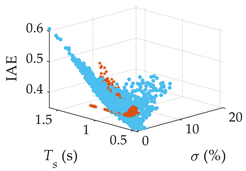 |
| G3(s) | 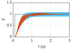 | 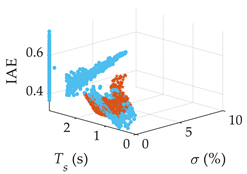 |
| G4(s) |  | 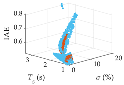 |
| G5(s) |  | 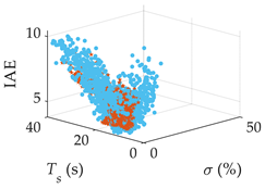 |
| G6(s) | 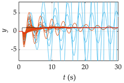 | 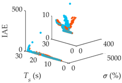 |
| Control Schemes | Parameters | |
|---|---|---|
| LQR | ωc = 45, ξ = 0.8 | Q = diag ([100 0]), R = 0.1 K = [31.6228 19.2195] |
| GCF-LQR | Kp = 8.5, Ki = 2.0, Kd = 6.4 | |
Disclaimer/Publisher’s Note: The statements, opinions and data contained in all publications are solely those of the individual author(s) and contributor(s) and not of MDPI and/or the editor(s). MDPI and/or the editor(s) disclaim responsibility for any injury to people or property resulting from any ideas, methods, instructions or products referred to in the content. |
© 2023 by the authors. Licensee MDPI, Basel, Switzerland. This article is an open access article distributed under the terms and conditions of the Creative Commons Attribution (CC BY) license (https://creativecommons.org/licenses/by/4.0/).
Share and Cite
Dai, C.; Gao, Z.; Chen, Y.; Li, D. Generalized Conditional Feedback System with Model Uncertainty. Processes 2024, 12, 65. https://doi.org/10.3390/pr12010065
Dai C, Gao Z, Chen Y, Li D. Generalized Conditional Feedback System with Model Uncertainty. Processes. 2024; 12(1):65. https://doi.org/10.3390/pr12010065
Chicago/Turabian StyleDai, Chengbo, Zhiqiang Gao, Yangquan Chen, and Donghai Li. 2024. "Generalized Conditional Feedback System with Model Uncertainty" Processes 12, no. 1: 65. https://doi.org/10.3390/pr12010065
APA StyleDai, C., Gao, Z., Chen, Y., & Li, D. (2024). Generalized Conditional Feedback System with Model Uncertainty. Processes, 12(1), 65. https://doi.org/10.3390/pr12010065