Multi-Step Prediction of Wind Power Based on Hybrid Model with Improved Variational Mode Decomposition and Sequence-to-Sequence Network

Abstract

Due to the complexity of wind power, traditional prediction models are incapable of fully extracting the hidden features of multidimensional strong fluctuation data, which results in poor multi-step prediction performance. To predict continuous power effectively in the future, an improved wind power multi-step prediction model combining variational mode decomposition (VMD) with sequence-to-sequence (Seq2Seq) is proposed. Firstly, the wind power sequence is smoothed using VMD and the decomposition parameters of VMD are optimized by using the squirrel search algorithm (SSA) to effectively optimize the decomposition effect. Then, the subsequence obtained from decomposition, together with the original wind power data, is reconstructed into multivariate time series features. Finally, a Seq2Seq model is constructed, and convolutional neural networks (CNNs) with bidirectional gate recurrent units (BiGRUs) are used to learn the coupling and timing relationships of the input data and encode them. The gate recurrent unit (GRU) is decoded to achieve continuous power prediction. Based on the actual operating data of a wind farm, a case analysis is conducted. Experimental results show that SSA-VMD can effectively optimize the decomposition effect, and the subsequences obtained with its decomposition are highly accurate when applied to predictions. The Seq2Seq model has better multi-step prediction results than traditional prediction methods, and as the prediction step size increases, the advantages are more obvious.

1. Introduction

In recent years, under the global consensus of building a clean, low-carbon energy system, the penetration of wind power in the power system has been increasing [1]. However, the uncertainty of wind power output poses a challenge to the operation control of the power system and restricts the large-scale grid-connected consumption of wind power [2,3]. Wind power prediction can provide a basis for grid scheduling, mitigate the disturbances in the power system caused by the wind power grid connection, and improve the utilization rate of wind power. It is also important for maintaining the security and stability of the grid and the operation and management of wind farms [4,5].

Wind turbines use the kinetic energy of wind to push the blades of the wind turbine to rotate the wind wheel and generate mechanical energy. The wind wheel drives the generator to run and convert kinetic energy into electrical energy. Wind power output is influenced by wind speed, temperature, humidity, and other factors. Wind power generation is highly volatile and intermittent due to meteorological and environmental factors, making it challenging to accurately predict wind power. A large amount of research has been conducted on this issue. The prediction can be classified into four categories based on different time scales: ultra-short-term (minutes to hours), short-term (hours to days), middle-term (weeks to months), and long-term (months to years) [6]. At this stage, wind power prediction methods can be divided into three categories: physical models, statistical models, and artificial intelligence models [7]. The physical model uses weather forecast data and geographical environment information to establish mathematical equations and makes predictions by describing the physical process of wind power conversion. However, physical model modeling has high complexity and requires a large amount of detailed information. It is suitable only for long-term prediction, and its application in short-term prediction is limited [8,9]. Statistical models use historical data to establish mathematical functions and fit the mapping relationships between them and predicted values, which are very suitable for short-term predictions. Commonly used statistical models include time series models, Kalman filter models, etc. [10,11]. However, the statistical model assumes that the time series is modeled in a linear form and cannot effectively handle the nonlinear characteristics of wind power data [12]. With the improvement in computer performance and the development of artificial intelligence technology, machine learning models have nonlinear feature learning capabilities and have been widely used in wind power prediction such as neural networks [13], support vector machines [14], etc. However, due to structural limitations, machine learning models are prone to fall into local optimality, overfitting, and poor convergence [15].

With the development of artificial intelligence, deep-learning methods have received wide attention in the prediction of new energy generation due to their stronger data mining ability. Peng et al. [16] and He et al. [17] use the convolutional neural network (CNN) and the deep confidence network, respectively, for wind power prediction, and find a large progress in prediction accuracy and stability. However, the time dependence of the input series is not taken into account. The variants of the recurrent neural network (RNN), such as long short-term memory (LSTM) and gated recurrent unit (GRU), can deal with temporal data features effectively and are suitable to be applied in the field of power prediction. Shi et al. [18] uses LSTM to perform hourly predictions of day-ahead wind power generation. Experimental results show that LSTM can achieve more accurate predictions than traditional neural networks. However, wind power is influenced by many factors, and the input of the prediction model is high-dimensional multivariable time series data. In many cases, variables in the multivariable time series data have spatiotemporal dependencies, and it is difficult for a single prediction method to effectively model the coupling information between the data [19].

Wind power is influenced by meteorological factors and has non-stationary fluctuation characteristics, which is the fundamental reason why wind power is difficult to predict. To solve this problem, the method of constructing a combined prediction model by combining data decomposition algorithms has been widely used and has become an important module to improve prediction performance. The power sequence is decomposed into several relatively stationary subsequences through the data decomposition method to reduce the impact of non-stationarity of the original power sequence on prediction. Xie et al. [20] uses wavelet decomposition to extract the time-frequency domain features of the power series, and then uses BiLSTM network for prediction. However, wavelet decomposition requires setting the wavelet basis function and the number of decompositions, and it lacks adaptivity. Wang et al. [21] proposed a wind power prediction model based on empirical mode decomposition (EMD) and a radial basis function neural network, and the results show that the prediction accuracy can be effectively improved using EMD decomposition. However, EMD is prone to the problem of modal aliasing. VMD can effectively avoid modal aliasing and is insensitive to noise [22]. It is currently the most effective decomposition method. Yildiz et al. [23] converts the subsequence obtained with variational mode decomposition (VMD) into spatial input feature maps, and then predicts wind power using a residual-based deep convolutional neural network. Aksan et al. [24] combines VMD and multiple deep-learning methods to form hybrid forecasting models, and these models show satisfactory applicability to load forecasting development scenarios under different conditions. However, the VMD decomposition parameters in references [23,24] all use empirical values. In practice, the VMD decomposition effect largely depends on the setting of the decomposition parameters. In the existing research, the value of K is usually determined with multiple experiments to select the optimal value or the central frequency method [25]. In addition, some researchers have introduced evaluation criteria such as information entropy [22] and energy [26] to objectively guide the value of K. However, the impact of the interaction between K and $\mathsf{\alpha }$ on the decomposition effect is not considered, and there is a lack of systematic evaluation standards to guide parameter setting [27].

Most of the existing studies are single-step predictions of power at a certain moment in the future, which cannot predict the power fluctuation trend and which provide limited information in practical applications. Multi-step prediction is capable of capturing the dynamic changes in future wind power to formulate and adjust the scheduling plan timely and appropriately and to promote the efficient and stable operation of the power system [28]. Because multi-step prediction is more complex than single-step prediction, more conditions need to be considered, such as error accumulation and prediction performance degradation [29]. Current multi-step prediction research on wind power mostly uses a data-driven approach to establish multi-step prediction models but fails to take into account the dependence between the prediction outputs. The sequence-to-sequence model is a sequential data modeling method that can generate an output sequence based on an input sequence, and the lengths of the input and output sequences do not affect each other. It has been widely used in tasks such as natural language processing and temporal data processing [30,31]. Multi-step prediction of wind power is essentially a sequence-to-sequence problem. The structure of the sequence-to-sequence model determines that it can handle well the input features and the prediction targets in multi-step prediction tasks.

Based on the above analysis, this paper combines the complementary advantages of data decomposition technology and deep-learning methods to propose a multi-step power prediction method based on improved VMD and Seq2Seq. The contributions and innovations of this paper are as follows:

• In order to solve the problem of VMD parameter setting, the average envelope entropy is introduced as an evaluation index, and the squirrel search algorithm is used to automatically find the optimal decomposition parameters of VMD to improve the decomposition effect. The original wind power sequence is preprocessed through SSA-VMD to enhance predictability.
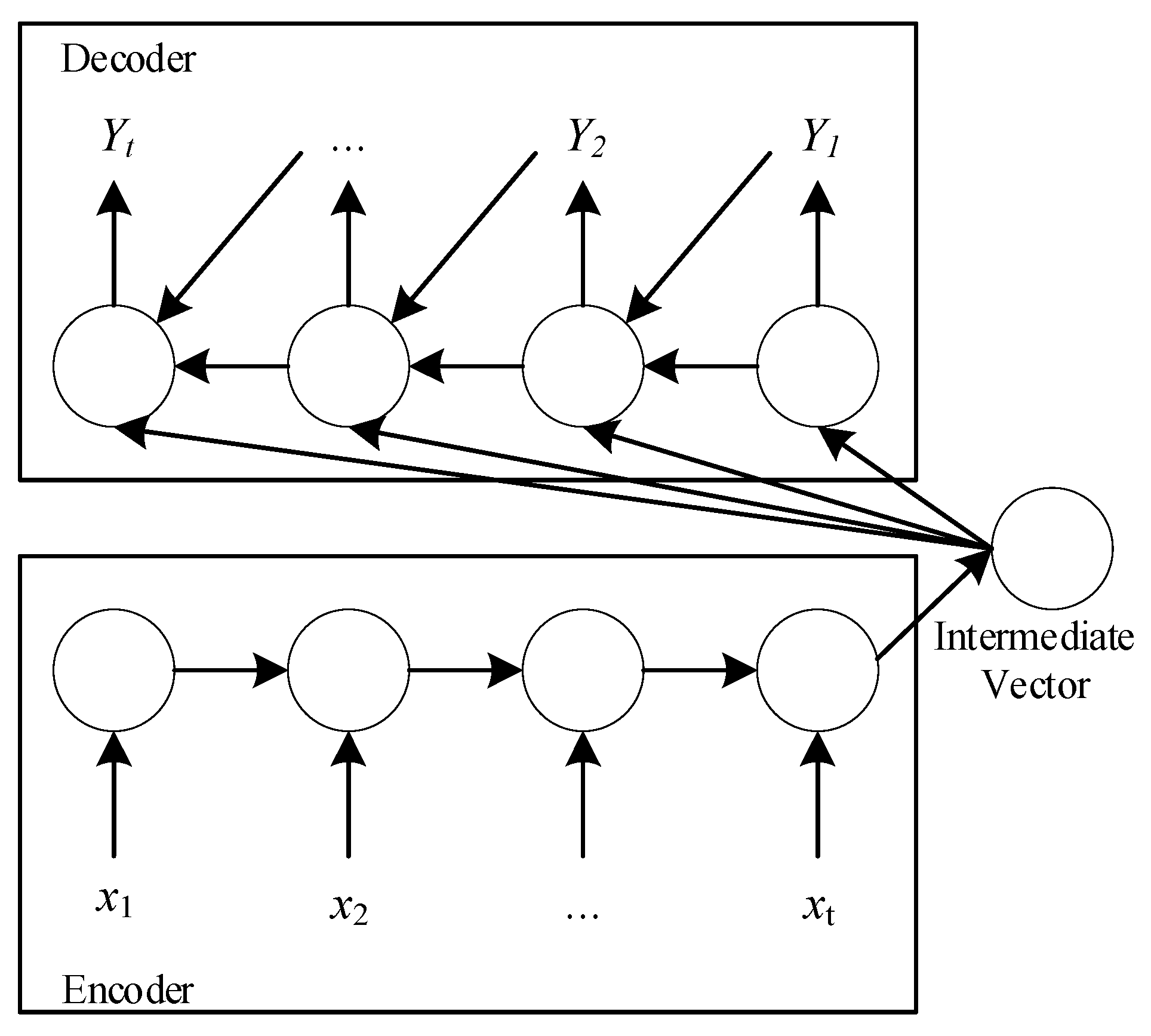
• A novel Seq2Seq model is proposed to be applied to the multi-step power prediction. The encoder encodes the hidden representation of the wind power time series data into context vectors, and the decoder progressively decodes the output prediction sequence. Through this end-to-end process, we can better learn the implicit correlation features of multidimensional time series data and achieve effective prediction of wind power power fluctuation trends in future time periods.
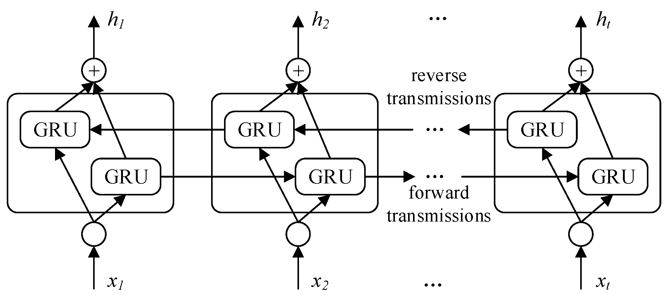
• Different from the traditional use of recurrent neural networks as the encoder and decoder of Seq2Seq, CNN-BiGRU is used as the encoder to extract the coupling information and timing information between the input data for encoding; the other GRU is used as the decoder to output predictions. The deep correlation information between the different features and the dependence between the time series data are fully explored.
• Finally, the effectiveness and robustness of the proposed model are proved by testing with the measured data set. The experimental results show that our model has the best prediction performance compared with the baseline method.

The rest of this paper is organized as follows. In Section 2, the principles and steps of the squirrel search algorithm for optimizing variational mode decomposition are elaborated. In Section 3, a brief description of the individual algorithms required for the proposed prediction model is presented. And then, in Section 4, the overall framework and details of the SSA-VMD-Seq2Seq model are provided. In Section 5, the experimental results and comparative examples of wind power prediction are discussed and the corresponding analysis is made. Finally, Section 6 serves as a summary of the paper.

2. SSA-VMD Algorithm

2.1. Variational Modal Decomposition

Variational mode decomposition (VMD) is an adaptive, non-completely recursive emerging signal processing method [32]. Its core is to decompose the original signal into several intrinsic mode functions (IMFs) with different bandwidth constraints and fluctuations around the center frequency. VMD mainly includes the construction of the variational problem and the solution of the variational problem in two parts [33]. The specific steps are as follows.

2.1.1. Variational Problem Construction

The signal to be decomposed is first decomposed into K modal components, and its resolved signals are computed using Hilbert transform to obtain the one-sided spectrum of each mode. Then, the spectrum of each mode is transferred to the corresponding fundamental frequency band, and the estimated bandwidth of each mode is obtained by solving the demodulated signal. The constrained variational problem of minimizing the sum of the estimated bandwidths of the IMFs is thus constructed:

$$\left\{\begin{array}{c}\underset{\left\{u_k\right\},\left\{{\omega }_k\right\}}{\min }\left\{\sum _{k=1}^K{‖{\mathit{\partial }}_t\left[\left(\delta \left(t\right)+\frac{j}{\mathsf{\pi }t}\right)\ast u_k\left(t\right)\right]e^{-j{\omega }_{k}t}‖}_2^2\right\}\\ \mathrm{s}.\mathrm{t}.\sum _{k=1}^K{u}_k=f\end{array}\right.,$$

(1)

where $u_k$ is the modal component, ${\omega }_k$ is the center frequency, K is the number of modal components, $\delta \left(t\right)$ is the Dirac function, and f is the original signal.

2.1.2. Variational Problem Solving

Next, introduce quadratic penalty terms and Lagrange multipliers to convert constrained variational problems into unconstrained variational problems. Construct the Lagrange multiplier function:

$$\begin{gathered} L\left(\left\{u_k\right\},\left\{{\omega }_k\right\},\lambda \right) \\ =\alpha \sum _k{‖{\mathit{\partial }}_t\left[\left(\delta \left(t\right)+\frac{j}{\mathsf{\pi }t}\right)\ast u_k\left(t\right)\right]e^{-j{\omega }_{k}t}‖}_2^2+{‖f\left(t\right)-\sum _k^{ }{u}_k\left(t\right)‖}^2 \\ +〈\lambda \left(t\right),f\left(t\right)-{\sum }_k{u}_k\left(t\right)〉. \end{gathered}$$

(2)

The alternating direction multiplier method is used for the solution, and $u_k$ and ${\omega }_k$ are updated by iteration to obtain the optimal solution with the iterative formula:

$$\left\{\begin{array}{c}{\widehat{u}}_k^{n+1}\left(\omega \right)=\frac{\widehat{f}\left(\omega \right)-\sum _{i\ne k}{\widehat{u}}_n^i\left(\omega \right)+\frac{{\widehat{\lambda }}^n\left(\omega \right)}{2}}{1+2\alpha {\left(\omega -{\omega }_n^k\right)}^2}\\ {\omega }_{n+1}^k=\frac{{\int }_0^{\infty }\omega {\left|{\widehat{u}}_k^{n+1}\left(\omega \right)\right|}^{2}d\omega }{{\int }_0^{\infty }{\left|{\widehat{u}}_k^{n+1}\left(\omega \right)\right|}^{2}d\omega }\end{array}\right.,$$

(3)

where ${\widehat{u}}_k^n\left(\omega \right)$, $\widehat{f}\left(\omega \right)$, and ${\widehat{\lambda }}^n\left(\omega \right)$ are the Fourier transformations of $u_k\left(\omega \right)$, $f\left(\omega \right)$, and ${\lambda }^n\left(\omega \right)$; n is the number of iterations.

2.2. Decomposition Performance Evaluation Criteria

K and $\alpha$ in the VMD decomposition parameters have a large impact on the decomposition effect. In power prediction applications, they are generally determined with empirical settings or the center frequency method [34]. However, due to the strong volatility of wind power series, the above two parameter setting methods are more subjective and random, and the decomposition is less effective. Therefore, the envelope entropy [35] is introduced as an evaluation criterion to guide the selection of VMD parameters. The envelope entropy is calculated as follows:

$$H_{en}\left(i\right)=-{\sum }_{n=1}^N{p}_i\left(n\right){\mathrm{l}\mathrm{o}\mathrm{g}}_2\left(p_i\left(n\right)\right),$$

(4)

where N is the number of sampling points and $p_i\left(n\right)$ is the normalized form of the envelope of the ith IMF component.

The size of the envelope entropy characterizes the sparsity of the signal. The smaller the entropy value, the higher the sparsity of the signal [36]. If the VMD parameter is selected more effectively, each mode will be more ordered, showing stronger sparsity; then, the envelope entropy value of each mode is the smallest. Under this condition, it indicates that the non-stationary characteristics of the original power series have been fully processed, and the great regularity of each subseries is conducive to high prediction accuracy. Therefore, in this paper, the average value of the envelope entropy of each modal component after decomposition is adopted as the fitness function, and the calculation formula is:

$$fitness=\underset{\left(K,\alpha \right)}{\min }\left\{\frac{1}{K}{\sum }_{i=1}^K{H}_{en}\left(i\right)\right\}.$$

(5)

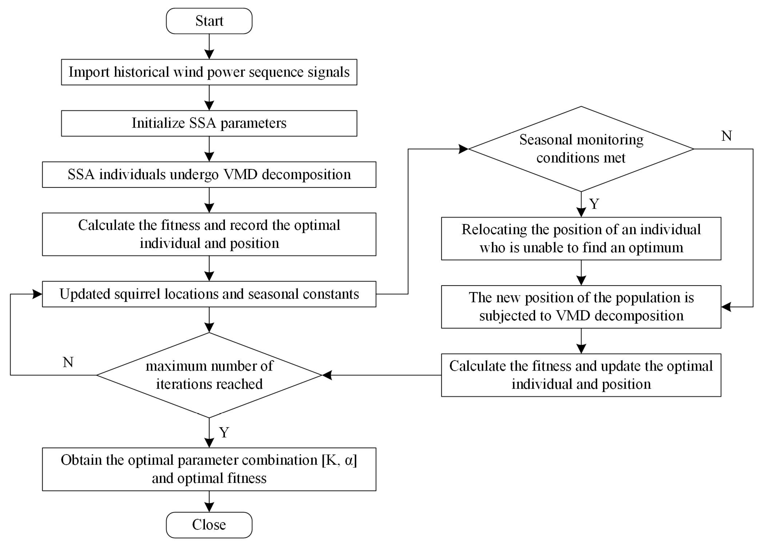
2.3. Squirrel Search Algorithm Optimized Variational Modal Decomposition

SSA is a relatively novel swarm intelligence optimization algorithm, which searches for the global optimal solution by simulating the dynamic foraging behaviors and movements of squirrels among different kinds of trees (hickory, oak, and common) in the forest. Reference [37] verifies the squirrel search algorithm on 33 classic optimization benchmark problems and compares it with 6 classic optimization algorithms such as the genetic algorithm and the particle swarm algorithm. Compared with other optimization algorithms, SSA has excellent convergence speed and exploration capabilities, as well as sufficient accuracy and robustness. Among the decomposition parameters of VMD, K determines the number of subsequences after decomposition; $\alpha$ determines the reconstruction accuracy of the signal. Therefore, the optimization dimension is set to 2, the VMD parameter selection problem is constructed as a constrained optimization problem, and SSA is used to solve this constrained optimization problem, which adaptively determines the optimal decomposition parameters and avoids the influence of parameter settings on the decomposition effect. The optimization flowchart is shown in Figure 1.

The specific steps are as follows:

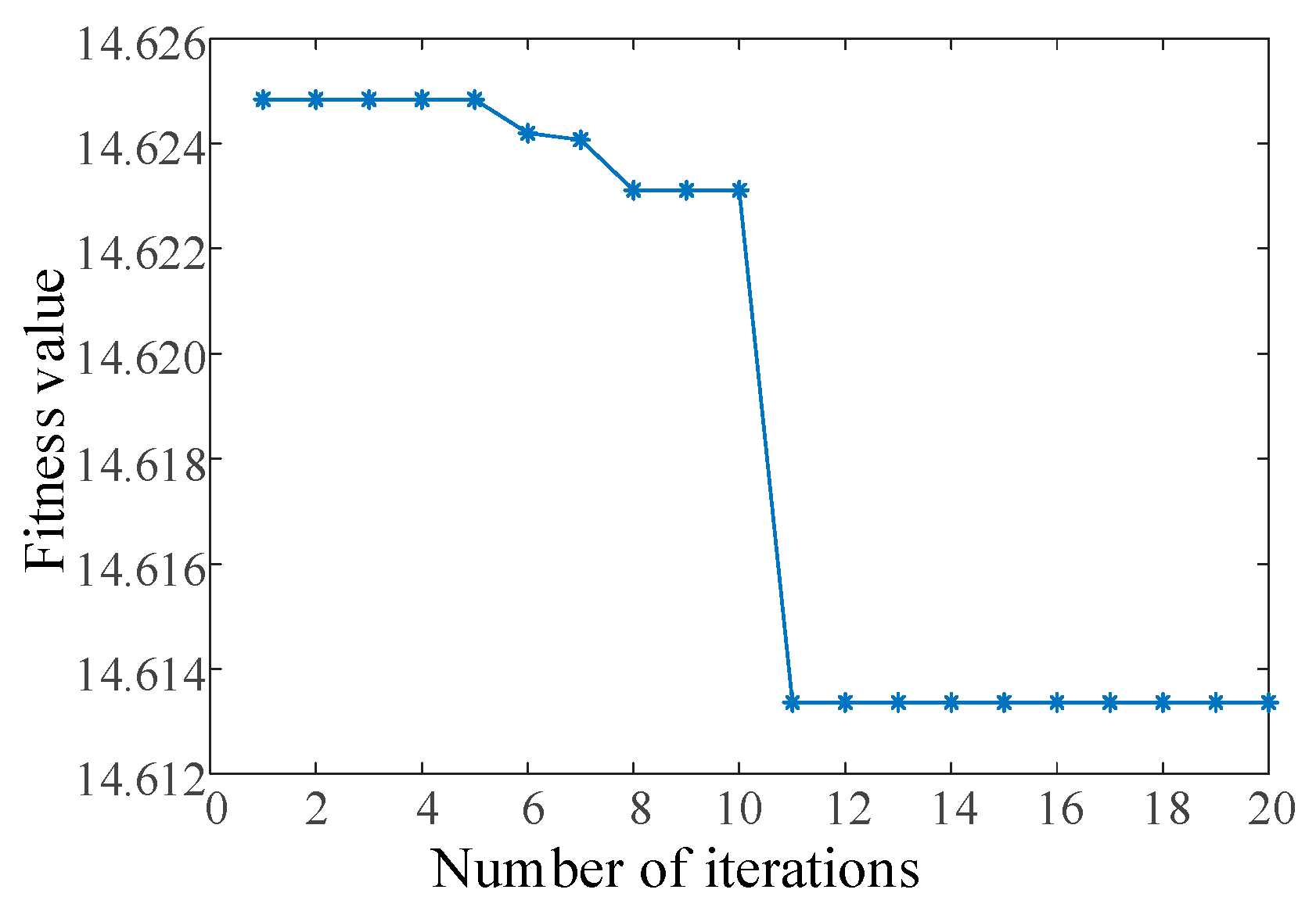
• Set the algorithm parameters and initialize the population position. The optimization dimension is 2, K and $\alpha$ are used as squirrel locations, and the two optimization search ranges are set to [3, 15] and [800, 2500], respectively. The population size is set to 20 and the maximum number of iterations is set to 20.
• Perform a VMD decomposition of the power sequence based on the location of each squirrel. Calculate the fitness of each individual and rank them. Assign the individual squirrels to the hickory tree (optimal food source), the oak tree (normal food source), and the common tree (no food source) in order to save the optimal individual squirrel positions.
• Update the individual squirrel locations. Three situations will occur based on the dynamic foraging behavior of squirrels: Situation 1, squirrels with normal food sources move to the optimal food source; Situation 2, squirrels with no food sources move to normal food sources; Situation 3, squirrels with no food sources move toward optimal food sources.
• Update the seasonal detection value, and when the seasonal detection value is less than the minimum seasonal constant, then randomly adjust the location of squirrels without a food source to re-forage.
• Calculate and rank the fitness of the new population and update the global optimal solution and the best fitness.
• Judge whether the maximum number of iterations is reached; if the judgement is no, repeat steps 3 to 5 until the maximum number of iterations is reached to end the optimization process. The location of squirrels on the optimal food source is the final optimal solution.

3. Principles of Predictive Modeling

3.1. Sequence-to-Sequence Fundamentals

Sequence-to-sequence (Seq2Seq) is a model in the field of deep learning that generates sequences from sequences without affecting each other in sequence length. It was first proposed by K. Cho et al. in 2014 and has been continuously improved [38]. Its core idea is to use an encoding–decoding structure to map a variable-length input sequence to a variable-length output sequence, which can flexibly handle tasks where the input sequence and output sequence are of different lengths. It has been widely used in fields such as machine translation [39,40], while there are still few applications in power prediction.

The basic structure of Seq2Seq is shown in Figure 2. It consists of two parts, the encoder and the decoder, and the information is passed between the two parts through the intermediate vectors. The encoder sequentially reads in the input sequence $x={\left[x_1,x_2,\dots ,x_t\right]}^T$ for compression coding to obtain a fixed-length intermediate vector and then maps and decodes the intermediate vector through the decoder to obtain the predicted output sequence $Y={\left[Y_1,Y_2,\dots ,Y_t\right]}^T$. The encoder and decoder are generally composed of a recurrent neural network, and the components of the encoder and decoder as well as the connection method can be selected according to the specific situation in practical applications [41].

3.2. Convolutional Neural Network

The convolutional neural network is a deep feedforward neural network with local connections, weight sharing, and other characteristics proposed by LeCun et al. [42]. CNN carries out deep processing of the input data through convolutional and pooling operations, extracts the key information in the data, and achieves dimensionality reduction, which significantly reduces the training parameters, reduces the computational complexity of the model, effectively learns the nonlinear local features in the input data, and improves the feature data quality. Therefore, feature extraction of multidimensional wind power data using CNN can help obtain deeper information about the wind power fluctuation law.

CNN mainly consists of an input layer, convolution layer, pooling layer, fully connected layer, and output layer [43]. The convolution layer uses a convolution kernel to sequentially scan each area on the data tensor and perform convolution operations to extract local feature information of the input data. The pooling layer performs dimensionality reduction on the feature data extracted by the convolutional layer to obtain the optimal output result. The abstract feature information obtained through the convolution layer and the pooling layer finally realizes the function of automatically learning features and streamlining from the original data. The calculation formula of the convolution operation is as follows [44]:

$$x_j^l=f\left({\sum }_{iϵM_j}{x}_i^{l-1}\ast k_{ij}^l+b_j^l\right),$$

(6)

where $x_j^l$ is the jth feature map of layer l, $f\left(\cdot \right)$ is the nonlinear activation function, $M_j$ is the jth feature map of layer $l-1$, $k_{ij}^l$ is the corresponding convolution kernel, $\ast$ is the convolution operation, and $b_j^l$ is the bias term.

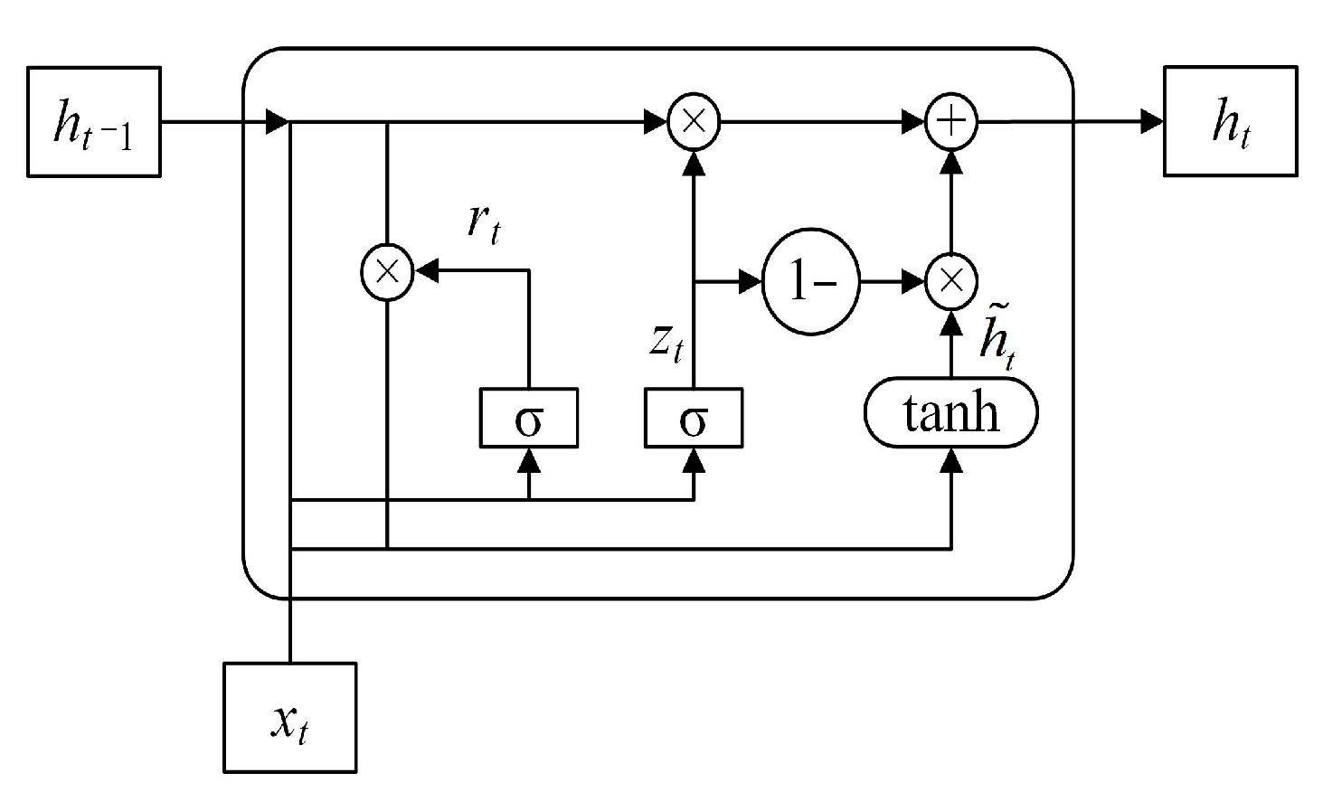
3.3. Bidirectional Gated Recurrent Unit

The GRU is a variant of the RNN, and the introduction of the gating mechanism improves the network structure, which retains the advantages of RNN in processing time-series data and at the same time improves the gradient explosion and gradient disappearance problems of RNN in processing long time sequences [45]. The gating structure and training parameters of GRU are more streamlined, which improves the computational efficiency under the premise of guaranteeing the prediction accuracy.

The basic unit structure of GRU is shown in Figure 3, where $x_t$ is the current moment input; $h_{t-1}$ and $h_t$ represent the implied layer states of the previous and current moments, respectively; ${\widehat{h}}_t$ is the candidate state of the current moment; $z_t$ is the update gate to control the retention degree of the historical state information and the current moment information; and $r_t$ is the reset gate to control the degree of combining of the current moment information and the historical state information. Furthermore, $h_t$ is the implied layer state of the GRU unit, which is calculated with Equation (7) [46]:

$$\left\{\begin{array}{c}{z}_t=\sigma \left(W_z{x}_t+U_z{h}_{t-1}+b_z\right)\\ r_t=\sigma \left(W_r{x}_t+U_r{h}_{t-1}+b_r\right)\\ \widetilde{h_t}=\mathit{tan}h\left(W_h{x}_t+U_h\left(r_t⨀h_{t-1}\right)+b_h\right)\\ h_t=z_t⨀h_{t-1}+\left(1-z_t\right)⨀\widetilde{h_t}\end{array}\right.,$$

(7)

where $W_z$, $W_r$, $U_z$, $U_r$, $W_h$, $U_h$ represent the weight matrix; $b_z$, $b_r$, $b_h$ are the bias vectors; $⨀$ is the pointwise multiplication operation; $\sigma$ is the sigmoid activation function; $tan$h is the hyperbolic tangent function.

BiGRU consists of a combination of two layers of GRUs that transfer information in forward and reversed time order, and the state of the implicit layer at each moment is jointly determined by the states of the two GRUs. Its network, unfolded in time order, is shown in Figure 4. BiGRU enhances the utilization of the original time series data, it can simultaneously utilize the feature information of the time series data in both the forward and backward directions, and it can improve the prediction accuracy efficiently. The calculation formula of the BiGRU model is as follows [47]:

$$\left\{\begin{array}{c}{\overrightarrow{h}}_t=\overrightarrow{f}\left(x_t,{\overrightarrow{h}}_{t-1}\right)\\ {\overleftarrow{h}}_t=\overleftarrow{f}\left(x_t,{\overleftarrow{h}}_{t-1}\right)\\ h_t={\overrightarrow{h}}_t⨁{\overleftarrow{h}}_t\end{array}\right.,$$

(8)

where ${\overrightarrow{h}}_{t-1}$ is the positive order implicit layer state, ${\overleftarrow{h}}_{t-1}$ is the negative order implicit layer state, and $⨁$ is the vector splicing operation.

4. SSA-VMD-Seq2Seq Prediction Model

In order to effectively predict the short-term multi-step power of wind farms, this paper proposes a wind power multi-step prediction model based on SSA-VMD-Seq2Seq. The output layer of the model has a step size of 16 to predict the power in the next 4 h. The model is based on the SSA-VMD-Seq2Seq model. The model mainly consists of four parts: SSA-VMD data decomposition, CNN local feature extraction, BiGRU temporal feature extraction coding, and GRU decoder prediction output to achieve end-to-end multi-step prediction. The overall framework of the model is shown in Figure 5.

4.1. Constructing Input Features

Firstly, the historical wind power series is decomposed using VMD. SSA is used to optimize the decomposition parameters of VMD during the decomposition process, and the power series is decomposed into several smoothed power subsequences and a residual sequence, highlighting the fluctuation characteristics of the subsequences in different frequency bands. After that, considering the dynamic influence of meteorological features on the output power, the decomposed subsequences together with the historical power and meteorological data sequences are spliced in the feature dimension and reconstructed into a multivariate time series feature map $X={\left[x_1,x_2,\dots ,x_T\right]}^T$, which has the dimensions of T × N, where T is the time step and N is the number of features (number of channels).

4.2. Encoding

In order to adapt to the model input with multivariate temporal features, the traditional Seq2Seq structure is improved. In this paper, CNN-BiGRU is used to construct the encoder, which combines the advantages of CNN in dealing with local features of multidimensional data and BiGRU in dealing with temporal features of sequential data and fully learns the implicit information of the input data for encoding.

The CNN contains one convolutional layer and one pooling layer. The convolutional layer is designed as a one-dimensional convolution, using a 1 × 1 convolutional kernel for the convolutional operation, which fuses the information of the input multidimensional features across channels and extracts the coupling relationships between different features at the same moment. In order to enhance the effective expression of the fused features, distinguishing from the conventional pooling, which is limited to only the operation of similar features in the spatial dimension, the pooling layer adopts the maximum pooling in the channel direction for the multi-channel fused features output from the 1 × 1 convolution kernel. After the above operations, the coupling information between different features is extracted and highlighted, and the original temporal correlation structure is preserved to obtain the deep fusion feature $Y={\left[y_1,y_2,\dots ,y_T\right]}^T$.

BiGRU is built as a two-layer structure to further learn the temporal change law and complete the encoding for the fusion features extracted with CNN. The input sequence is input sequentially in chronological order, and after T time steps of updating, the implicit layer state $h_T$ at the last moment is obtained by encoding. Theoretically, $h_T$ contains all the information of the input sequence, which is passed to the decoder as the intermediate state vector c obtained by encoding, and its expression is:

$$c=h_T=BiGRU\left(h_{T-1},y_T\right),$$

(9)

where $h_{T-1}$ is the state of the hidden layer at the moment $T-1$ and $y_T$ is the feature at the Tth time step in the input sequence.

4.3. Decoding

The decoder consists of a single-layer GRU. The initial implicit state of the GRU is the intermediate state vector c. The predicted power sequences are generated by the decoder one by one in time order. In the step-by-step decoding process, at each moment, the GRU unit accepts the implied layer state $h_{T-1}$ of the previous moment, the intermediate state vector c, and the power prediction value $P_{T+t-1}^{\prime }$, output from the previous moment (the first moment is the real power value $P_T$ at the moment of T) to update the current implied layer state, and outputs the current power prediction value through the fully connected layer with the expression:

$$\left\{\begin{array}{c}{h}_t=f\left(G\left[h_{t-1},P_{T+t-1}^{\prime },c\right]+b_h\right)\\ P_{T+t}^{\prime }=g\left(V{h}_t+b_o\right)\end{array}\right.,$$

(10)

where G, V represent the weight matrix; $b_h$, $b_o$ represent the bias vector; and f, g represent the activation function. After the above process, the sharing of coded feature information on step-by-step decoding is achieved, and the temporal relationship between successive predicted outputs is taken into account to complete the power prediction from the input features of the previous T time steps for the next t time steps.

5. Case Study

5.1. Description of the Experiment

The experimental data is sourced from the wind power plant in Hami City, Xinjiang Province, China, for the entire year of 2019, comprising actual wind power measurements and meteorological observation data. The sampling interval is 15 min, totaling 35,040 data points. The wind farm consists of 133 turbines, each with a capacity of 1.5 MW, resulting in a total installed capacity of 200 MW. Meteorological observation data include wind speed and wind direction at heights of 10 m, 30 m, 50 m, and 70 m (hub height) as well as temperature, humidity, and air pressure, making up a total of 11 meteorological features. To mitigate the impact of data quality on modeling effectiveness, a correlation analysis was conducted using the maximum information coefficient method [47]. Two strongly correlated meteorological factors, namely, wind speed and wind direction at 70 m, along with historical power, were selected as input features for modeling. A sliding window approach was employed to construct supervised learning-formatted sample data, which was then divided into training, validation, and test sets in a 6:2:2 ratio for simulation analysis.

The model in this paper is constructed based on Python 3.9 using the TensorFlow 2.8 deep-learning framework. During the training phase, the hyperparameter configuration in deep-learning models is crucial for adjusting and optimizing the model’s behavior and performance. There is no fixed answer for setting hyperparameters in deep-learning models; it involves systematic experimentation, adherence to best practices, and leveraging domain knowledge [24]. In this paper, repeated experiments were conducted based on a large number of previous references to draw conclusions on a reasonable setting of network parameters. The input timing length was set to 32; in the encoder, the number of convolution kernels was 32 (Predicting the future 16 time points within the next 4 h with the same 15-min interval is based on utilizing 32 historical data points sampled at 15-min intervals from the preceding 8 h as input features), the pooling size was 2, and the number of implied nodes of the BiGRU was 64; in the decoder, the number of implied nodes of the GRU was 64 and the number of neurons of the fully-connected layer was 64. The number of neurons was 64. The learning rate was set to 0.001 in the hyperparameters for model training; the batch size was 256, and the number of training rounds was 100.

In order to evaluate the model prediction results objectively, mean absolute error (MAE), root-mean-square error (RMSE), and mean absolute percentage error (MAPE) were selected as the evaluation indicators. MAE reflects the average deviation between predicted and actual values [48], while RMSE not only reveals the bias between predicted and actual values but also shows their dispersion [49]. MAPE, on the other hand, reflects the average percentage difference between predicted and actual values [50]. Smaller values of MAE, RMSE, and MAPE indicate better performance of the predictive model. The mathematical formulas for these error metrics are as follows:

$$MAE=\frac{1}{N}{\sum }_{i=1}^N\left|{\widehat{y}}_i-y_i\right|,$$

(11)

$$RMSE=\sqrt{\frac{1}{N}{\sum }_{i=1}^N{\left({\widehat{y}}_i-y_i\right)}^2},$$

(12)

$$MAPE=\frac{1}{N}{\sum }_{i=1}^N\left|\frac{{\widehat{y}}_i-y_i}{y_i}\right|\times 100\%,$$

(13)

where N is the number of samples, ${\widehat{y}}_i$ is the predicted value of the ith sample, and $y_i$ is the true value of the ith sample.

5.2. SSA-VMD Effect and Prediction Experiments

In addressing the issue of preset parameter selection for the VMD algorithm, this section employs the minimum average envelope entropy as an evaluation criterion. Utilizing the SSA algorithm, the two parameters of the VMD are optimized, as illustrated in Figure 6. By the 11th iteration, the fitness reaches the minimum value of 14.6134, converging to the global optimum. Simultaneously, the optimal decomposition parameters for VMD are determined as K = 8, $\mathsf{\alpha }=1265$. Using the optimized parameters, VMD decomposition is applied to the historical power sequence, as shown in Figure 7. From IMF1 to IMF8, the average amplitude of the subsequences gradually decreases, while the volatility increases. This indicates that VMD decomposition effectively mitigates the volatility and non-stationarity of the original power sequence, with each subsequence reflecting the changing characteristics of wind power in different frequency bands and time scales.

In order to verify the effectiveness of the SSA-optimized VMD parameters, the original data without decomposition, the VD with default parameters (K = 1000, $\mathsf{\alpha }=5$), the CF-VMD (K = 1000, $\mathsf{\alpha }=10$) using the center frequency method (denoted as CF), and the subsequence data obtained from the three decomposition algorithms of the SSA-VMD were fed into the Seq2Seq model for single-step prediction. The prediction results of each method are shown in Figure 8, and

Table 1. Comparison of prediction errors under different decomposition methods.

Decomposition Methods	MAE/MW	RMSE/MW	MAPE/%
Undecomposed	4.155	6.985	15.886
VMD	2.19	3.174	12.508
CF-VMD	1.865	2.274	12.89
SSA-VMD	1.104	1.542	9.662

shows the comparison of the prediction evaluation indexes.

As shown in Table 1 and Figure 8, compared with the undecomposed method, the three decomposed methods have reduced the MAE, RMSE, and MAPE of the model prediction results and mitigated the latency issue. This indicates the effectiveness of the variational mode decomposition (VMD) algorithm in improving prediction accuracy. In comparison with the VMD method with default values, the model’s predictive performance improved after the VMD parameters were determined through the central frequency method and singular spectrum analysis (SSA). The RMSE decreased by 0.9 and 1.632, highlighting the necessity of optimizing VMD decomposition parameters. Among the four methods, the model using SSA-VMD decomposition exhibited the optimal performance, with MAE, RMSE, and MAPE values of 1.104, 1.542, and 9.662, respectively. These metrics suggest that SSA-VMD, when compared with VMD parameters determined using the central frequency method, achieves better decomposition results. When combined with the predictive model, the SSA-VMD method demonstrates superior predictive performance, with prediction results closely aligning with actual power fluctuations.

5.3. Seq2Seq Encoding–Decoding Structure Ablation Experiments

The selection of encoders and decoders in the Seq2Seq model has greater flexibility and directly affects the prediction performance. This paper proposes a new Seq2Seq structure, in which the encoder uses CNN-BiGRU and the decoder uses GRU. In order to verify the superiority of the proposed Seq2Seq structure, a series of ablation experiments was conducted and a detailed analysis of the network structure was carried out.

In previous research, the encoder and decoder of the Seq2Seq model were usually composed of recurrent neural networks. Therefore, LSTM, GRU, and BiGRU were designed as encoders, and different decoder network structures were constructed accordingly. The input features of the prediction model all use multivariate time series decomposed with SSA-VMD. To compare with the Seq2Seq structure proposed in this paper, the prediction performance was evaluated at 4 steps (1 h), 8 steps (2 h), and 16 steps (4 h) ahead.

Table 2. Comparison of prediction errors under different encoding–decoding structures.

Modeling		Predicted Step Length	MAE /MW	RMSE /MW	MAPE /%
Encoders	Decoders
LSTM	LSTM	4 steps	2.726	4.36	15.031
		8 steps	3.023	4.703	17.345
		16 steps	4.382	6.401	31.514
GRU	GRU	4 steps	2.819	4.036	23.809
		8 steps	2.552	3.916	15.455
		16 steps	5.176	6.99	47.67
BiGRU	GRU	4 steps	2.036	3.199	11.252
		8 steps	2.543	3.832	13.279
		16 steps	4.709	6.368	39.765
CNN- BiGRU	GRU	4 steps	1.902	3.02	10.73
		8 steps	2.409	3.681	12.589
		16 steps	3.616	5.366	20.527

shows the prediction errors under different structures.

As shown in Table 2, the impact of each module of this paper’s structure on performance improvement can be seen. In the classic Seq2Seq model structure composed of recurrent neural networks, the prediction index of both the encoder and the decoder being GRU is generally better than that of the structure where the encoder and decoder are both LSTM. At the same time, GRU has one less gate than the LSTM mechanism, with fewer network parameters and higher computational efficiency. A bidirectional mechanism is introduced on the basis of GRU. When the BiGRU is used as an encoder, the MAE and MAPE at four and eight steps in advance are significantly reduced, indicating that through bidirectional timing data processing, the timing characteristics of wind power sequences can be more effectively captured. After further integrating CNN to form the CNN-BiGRU encoder, MAE, RMSE, and MAPE are all the lowest compared with other models, which shows that CNN can effectively extract the coupling relationship between multivariable time series data and make up for BiGRU’s deficiencies in processing high-dimensional data. In summary, the necessity and effectiveness of the model structure design in this article have been proved through the ablation experiment of the network structure.

5.4. Experiments on Multi-Step Prediction Performance of the Seq2Seq Model

To assess the performance of the proposed Seq2Seq model in multi-step prediction, this section uses SSA-VMD processed multivariate time series as input and compares its multi-step prediction performance with four influential benchmark models in the field of wind power prediction. These models are the classic shallow-learning models MLP and SVR as well as two benchmark deep-learning models, CNN and LSTM. Detailed descriptions of these models are provided below.

In terms of model input requirements, CNN, LSTM, and Seq2Seq models can receive 3D arrays, and the input data structure is [sample, time step, feature]. MLP and SVR need to receive 2D arrays as input. In order to meet the requirements, the data preprocessing stage converts the 3D array into a 2D array, and the structure is expressed as [sample, time step ∗ feature]. In terms of multi-step prediction strategies, the structure of Seq2Seq can flexibly process model output and gradually output multi-step prediction results. For the four benchmark models, the three models of MLP, CNN, and LSTM modify the network structure and modify the original output layer into a fully connected layer with a number of connected neurons equal to the length of the prediction time for complete field multi-step prediction. However, SVR has a unique output due to the limitations of the model principle. It is necessary to establish a separate prediction model for each prediction step to achieve multi-step prediction. In terms of model parameter settings, the benchmark should be kept consistent, and the same configuration parameters need to be used in different deep-learning models to ensure consistency in analyzing two key parameters: the accuracy and stability of the prediction model.

Table 3. Comparison of multi-step prediction errors for different prediction models.

Modeling	Predicted Step Length	MAE/MW	RMSE/MW	MAPE/%
MLP	4 steps	3.451	4.811	25.005
	8 steps	6.44	8.024	59.391
	16 steps	7.782	10.816	68.974
SVR	4 steps	5.081	6.777	59.782
	8 steps	5.881	7.504	71.971
	16 steps	6.538	8.525	68.155
CNN	4 steps	2.673	3.884	19.553
	8 steps	3.628	5.106	30.979
	16 steps	6.531	9.059	58.595
LSTM	4 steps	3.51	4.88	29.026
	8 steps	3.01	4.626	15.439
	16 steps	5.465	7.712	22.924
Seq2Seq	4 steps	1.902	3.02	10.73
	8 steps	2.409	3.681	12.589
	16 steps	3.616	5.366	20.527

and Figure 9 show the comparison of prediction errors and prediction results of different prediction models with 4 steps (1 h), 8 steps (2 h), and 16 steps (4 h) in advance, respectively. The following conclusions were obtained from the comparative analysis:

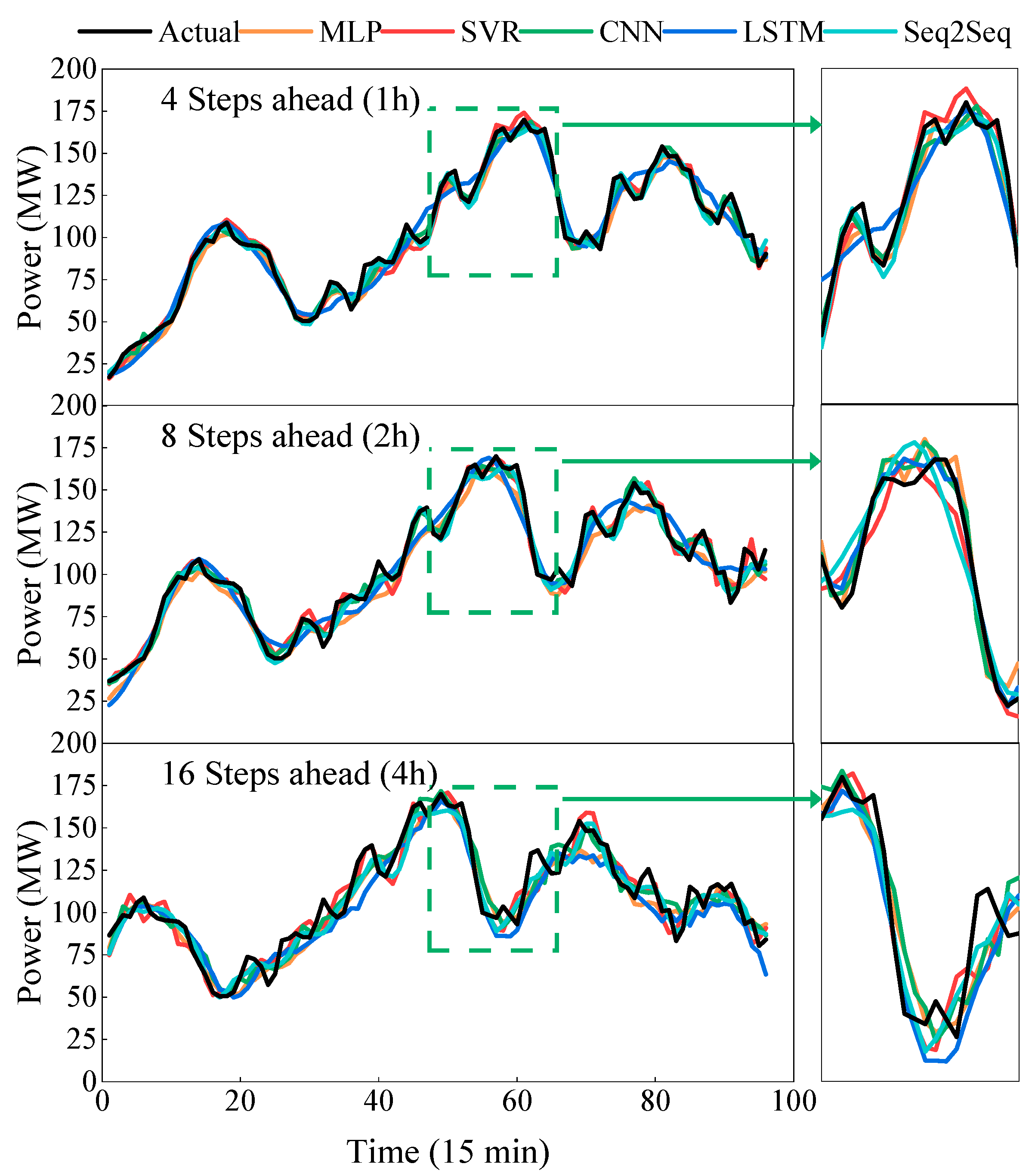
• As the prediction step size increases, the error metrics of all models increase. This shows that the longer the prediction time step is, the more obvious the cumulative error of the model will be, and the more difficult the prediction will be. Among them, the Seq2Seq model is least affected. The MAE, RMSE, and MAPE of the 16-step-ahead prediction are increased by 50.10%, 45.77%, and 63.06%, respectively, compared with the 8-step-ahead prediction. The prediction error increases minimally compared with the baseline method.
• When wind power generation experiences non-stationary fluctuations, the prediction curves of MLP, SVR, and CNN exhibit pronounced oscillations, indicating unstable predictive performance. In contrast, the prediction curves of LSTM and Seq2Seq are relatively smooth. Specifically, Seq2Seq demonstrates MAPE values of 10.73, 12.589, and 20.527 for lead time predictions of 4, 8, and 16 steps, respectively. This suggests that the Seq2Seq model is less affected by data fluctuations, resulting in more stable predictive performance and a closer fit to actual power fluctuations.
• The Seq2Seq model has the lowest MAE, RMSE, and MAPE at 4 steps, 8 steps, and 16 steps in advance, and the advantages become more obvious as the prediction step size increases; the prediction accuracy is the highest. Experimental results show that the Seq2Seq model can maintain the lowest prediction error compared with the baseline method, and the prediction results are more accurate.

6. Conclusions

To effectively predict continuous power for future time periods and enhance the referential value of the predictions, this paper combined data decomposition techniques with deep-learning methods and proposed an improved VMD- and Seq2Seq-based wind power multi-step prediction model. The following conclusions are drawn from the simulation results:

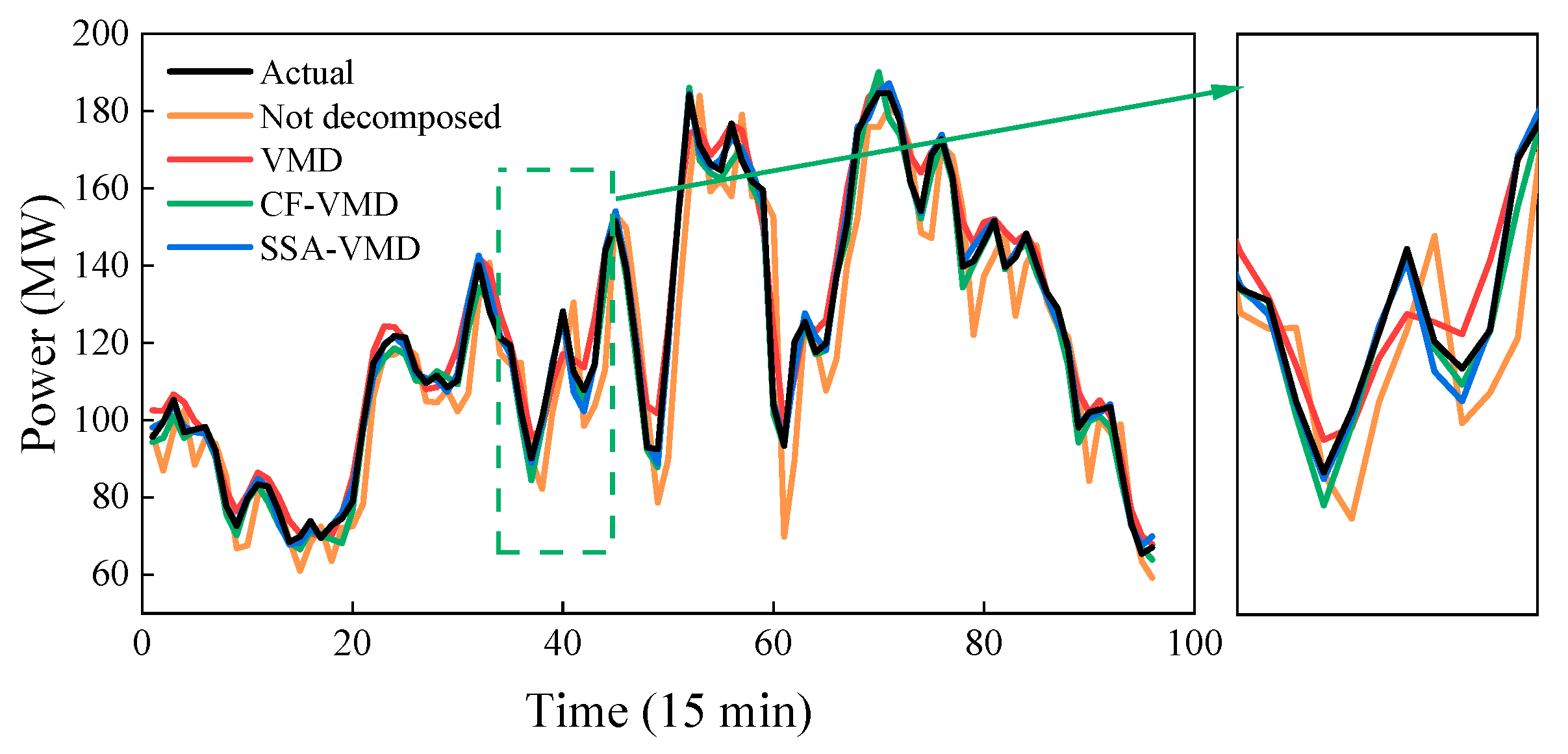
• The optimization of VMD decomposition parameters through SSA successfully improves the decomposition effectiveness for wind power sequences. The resulting subsequences exhibited stronger representation capabilities of the feature information. In comparison with the traditional approach of determining VMD decomposition parameters using the central frequency method, SSA-VMD reduced the randomness associated with empirical settings and led to higher accuracy in predictions.
• The introduction of CNN-BiGRU as the encoder for the Seq2Seq model fully utilized CNN to extract coupling information between multivariate time series and further exploited deep temporal features through BiGRU. This improvement enhances the model’s encoding capabilities, making it more sensitive to changes in key features.
• The Seq2Seq model proposed in this paper demonstrates significant advantages in multi-step predictions, particularly as the time step increases. Owing to its unique compression–encoding–decoding mechanism, the model delves deeply into uncovering the changing characteristics of wind power. Additionally, the decoder adopts an output feedback mode to predict continuous power sequences, reducing the impact of error accumulation.
• Compared with other benchmark models, the proposed hybrid prediction approach performs best in advance predictions at various lead times, with optimal values achieved for RMSE, MAE, and MAPE metrics. This indicates that the proposed method significantly enhances prediction accuracy and robustness, demonstrating a certain level of applicability.

Lastly, there is still room for improvement in this approach. Because the setting of model hyperparameters is crucial for predictive performance, future research could involve optimizing model hyperparameters through the integration of heuristic algorithms to enhance predictive capabilities. Additionally, building upon the foundation of this study, sensitivity analysis, validation, and benchmark testing will be necessary to verify the generalization performance of the proposed model. This will further explore its broader applications in the wind power domain.

References

1. Kisvari, A.; Lin, Z.; Liu, X. Wind power forecasting—A data-driven method along with gated recurrent neural network. Renew. Energy 2021, 163, 1895–1909. [Google Scholar] [CrossRef]
2. Cui, Y.; Chen, Z.H.; Liu, L.J. Short-term wind power prediction analysis of complicated topography in abandoned wind power conditions. Acta Energiae Solaris Sin. 2017, 38, 3376–3384. [Google Scholar]
3. Dong, Y.; Zhang, H.; Wang, C.; Zhou, X. A novel hybrid model based on Bernstein polynomial with mixture of Gaussians for wind power forecasting. Appl. Energy 2021, 286, 116545. [Google Scholar] [CrossRef]
4. Yang, M.; Zhou, Y. Ultra-short-term prediction of wind power considering wind farm status. Proc. CSEE 2019, 39, 1259–1268. [Google Scholar]
5. Hossain, M.A.; Chakrabortty, R.K.; Elsawah, S.; Ryan, M.J. Very short-term forecasting of wind power generation using hybrid deep learning model. J. Clean. Prod. 2021, 296, 126564. [Google Scholar] [CrossRef]
6. Zhou, X.; Liu, C.; Luo, Y.; Wu, B.; Dong, N.; Xiao, T.; Zhou, H. Wind power forecast based on variational mode decomposition and long short term memory attention network. Energy Rep. 2022, 8, 922–931. [Google Scholar] [CrossRef]
7. Qian, Z.; Pe, Y.; Cao, L.X.; Wang, J.Y.; Jing, B. Review of wind power forecasting method. High Volt. Eng. 2016, 42, 1047–1060. [Google Scholar]
8. Feng, S.L.; Wang, W.S.; Liu, C.; Dai, H.Z. Study on the physical approach to wind power prediction. Proc. CSEE 2010, 30, 1–6. [Google Scholar]
9. Wang, H.; Han, S.; Liu, Y.; Yang, J.; Li, L. Sequence transfer correction algorithm for numerical weather prediction wind speed and its application in a wind power forecasting system. Appl. Energy 2019, 237, 1–10. [Google Scholar] [CrossRef]
10. Liu, S.; Zhu, Y.L.; Zhang, K.; Gao, J.C. Short term wind power forecasting based on error correction ARMA-GARCH model. Acta Energiae Solaris Sin. 2020, 41, 268–275. [Google Scholar]
11. Guan, C.; Luh, P.B.; Michel, L.D.; Chi, Z. Hybrid Kalman filters for very short-term load forecasting and prediction interval estimation. IEEE Trans. Power Syst. 2013, 28, 3806–3817. [Google Scholar] [CrossRef]
12. Song, J.; Wang, J.; Lu, H. A novel combined model based on advanced optimization algorithm for short-term wind speed forecasting. Appl. Energy 2018, 215, 643–658. [Google Scholar] [CrossRef]
13. Wang, Z.; Wang, B.; Liu, C.; Wang, W. Improved BP neural network algorithm to wind power forecast. J. Eng. 2017, 2017, 940–943. [Google Scholar] [CrossRef]
14. Lu, P.; Ye, L.; Tang, Y.; Zhao, Y.; Zhong, W.; Qu, Y.; Zhai, B. Ultra-short-term combined prediction approach based on kernel function switch mechanism. Renew. Energy 2021, 164, 842–866. [Google Scholar] [CrossRef]
15. Khodayar, M.; Wang, J.; Manthouri, M. Interval deep generative neural network for wind speed forecasting. IEEE Trans. Smart Grid 2018, 10, 3974–3989. [Google Scholar] [CrossRef]
16. Peng, X.; Li, Y.; Dong, L.; Cheng, K.; Wang, H.; Xu, Q.; Wang, B.; Liu, C.; Che, J.; Yang, F.; et al. Short-term wind power prediction based on wavelet feature arrangement and convolutional neural networks deep learning. IEEE Trans. Ind. Appl. 2021, 57, 6375–6384. [Google Scholar] [CrossRef]
17. He, J.J.; Yu, C.J.; Li, Y.L.; Xiang, H.Y. Ultra-short term wind prediction with wavelet transform, deep belief network and ensemble learning. Energy Convers. Manag. 2020, 205, 112418. [Google Scholar]
18. Shi, X.; Lei, X.; Huang, Q.; Huang, S.Z.; Ren, K.; Hu, Y.Y. Hourly day-ahead wind power prediction using the hybrid model of variational model decomposition and long short-term memory. Energies 2018, 11, 3227. [Google Scholar] [CrossRef]
19. Du, S.; Li, T.; Yang, Y.; Horng, S.J. Multivariate time series forecasting via attention-based encoder–decoder framework. Neurocomputing 2020, 388, 269–279. [Google Scholar] [CrossRef]
20. Xie, X.Y.; Zhou, J.H.; Zhang, Y.J.; Wang, J.; Su, J.Y. W-BilSTM based ultra-short-term generation power predictionmethod of renewable energy. Autom. Electr. Power Syst. 2021, 45, 175–184. [Google Scholar]
21. Wang, J.X.; Deng, B.; Wang, J. Short-term wind power prediction based on empirical mode decomposition and RBF neural network. J. Electr. Power Syst. Autom. 2020, 32, 109–115. [Google Scholar]
22. Duan, J.; Wang, P.; Ma, W.; Tian, X.; Fang, S.; Cheng, Y.; Chang, Y.; Liu, H. Short-term wind power forecasting using the hybrid model of improved variational mode decomposition and Correntropy Long Short-term memory neural network. Energy 2021, 214, 118980. [Google Scholar] [CrossRef]
23. Yildiz, C.; Acikgoz, H.; Korkmaz, D.; Budak, U. An improved residual-based convolutional neural network for very short-term wind power forecasting. Energy Convers. Manag. 2021, 228, 113731. [Google Scholar] [CrossRef]
24. Aksan, F.; Suresh, V.; Janik, P.; Sikorski, T. Load Forecasting for the Laser Metal Processing Industry Using VMD and Hybrid Deep Learning Models. Energies 2023, 16, 5381. [Google Scholar] [CrossRef]
25. Zhang, G.; Liu, H.; Zhang, J.; Yan, Y.; Zhang, L.; Wu, C.; Hua, X.; Wang, Y. Wind power prediction based on variational mode decomposition multi-frequency combinations. J. Mod. Power Syst. Clean Energy 2019, 7, 281–288. [Google Scholar] [CrossRef]
26. Zhang, Y.; Li, R.; Zhang, J. Optimization scheme of wind energy prediction based on artificial intelligence. Environ. Sci. Pollut. Res. 2021, 28, 39966–39981. [Google Scholar] [CrossRef] [PubMed]
27. Wang, Y.; Wu, L. On practical challenges of decomposition-based hybrid forecasting algorithms for wind speed and solar irradiation. Energy 2016, 112, 208–220. [Google Scholar] [CrossRef]
28. Fu, W.; Wang, K.; Li, C.; Tan, J. Multi-step short-term wind speed forecasting approach based on multi-scale dominant ingredient chaotic analysis, improved hybrid GWO-SCA optimization and ELM. Energy Convers. Manag. 2019, 187, 356–377. [Google Scholar] [CrossRef]
29. Bao, Y.; Xiong, T.; Hu, Z. Multi-step-ahead time series prediction using multiple-output support vector regression. Neurocomputing 2014, 129, 482–493. [Google Scholar] [CrossRef]
30. Tang, J.; Hou, H.J.; Chen, H.G.; Wang, S.J.; Sheng, G.H.; Jiang, C.X. Concentration prediction method based on Seq2Seg network improved by BI-GRU for dissolved gas intransformer oil. Electr. Power Autom. Equip. 2022, 42, 196–202+217. [Google Scholar]
31. Deng, Y.; Wang, L.; Jia, H.; Tong, X.; Li, F. A sequence-to-sequence deep learning architecture based on bidirectional GRU for type recognition and time location of combined power quality disturbance. IEEE Trans. Ind. Inform. 2019, 15, 4481–4493. [Google Scholar] [CrossRef]
32. Dragomiretskiy, K.; Zosso, D. Variational mode decomposition. IEEE Trans. Signal Process. 2013, 62, 531–544. [Google Scholar] [CrossRef]
33. Jing, X.; Luo, J.; Zhang, S.; Wei, N. Runoff forecasting model based on variational mode decomposition and artificial neural networks. Math. Biosci. Eng. 2022, 19, 1633–1648. [Google Scholar] [CrossRef] [PubMed]
34. Yang, J.X.; Zhang, S.; Liu, J.C.; Liu, J.Y.; Xiang, Y.; Han, X.Y. Short-term photo-voltaic power prediction based on variational mode decomposition and long short term memory with dual-stage attention mechanism. Autom. Electr. Power Syst. 2021, 45, 174–182. [Google Scholar]
35. Li, H.; Fan, B.; Jia, R.; Zhai, F.; Bai, L.; Luo, X.Q. Research on multi-domain fault diagnosis of gearbox of wind turbine based on adaptive variational mode decomposition and extreme learning machine algorithms. Energies 2020, 13, 1375. [Google Scholar] [CrossRef]
36. Yao, J.; Xiang, Y.; Qian, S.; Wang, S.; Wu, S. Noise source identification of diesel engine based on variational mode decomposition and robust independent component analysis. Appl. Acoust. 2017, 116, 184–194. [Google Scholar] [CrossRef]
37. Jain, M.; Singh, V.; Rani, A. A novel nature-inspired algorithm for optimization: Squirrel search algorithm. Swarm Evol. Comput. 2019, 44, 148–175. [Google Scholar] [CrossRef]
38. Cho, K.; Van Merriënboer, B.; Gulcehre, C.; Bahdanau, D.; Bougares, F.; Schwenk, H.; Bengio, Y. Learning phrase representations using RNN encoder-decoder for statistical machine translation. arXiv 2014, arXiv:1406.1078. [Google Scholar]
39. Sutskever, I.; Vinyals, O.; Le, Q.V. Sequence to sequence learning with neural networks. Adv. Neural Inf. Process. Syst. 2014, 27, 3104–3112. [Google Scholar]
40. Kuznetsov, V.; Mariet, Z. Foundations of sequence-to-sequence modeling for time series. arXiv 2018, arXiv:1805.03714. [Google Scholar]
41. Chen, Y.C.; Zhang, D.H.; Yu, H.; Wang, Y.Q. Short-term Bus Load Forecasting of Multi Feature Based on Seq2seq Model. J. Electr. Power Syst. Autom. 2023, 35, 1–6+35. [Google Scholar]
42. LeCun, Y.; Boser, B.; Denker, J.S.; Henderson, D.; Howard, R.E.; Hubbard, W.; Jackel, L.D. Backpropagation applied to handwritten zip code recognition. Neural Comput. 1989, 1, 541–551. [Google Scholar] [CrossRef]
43. Ghosh, A.; Sufian, A.; Sultana, F.; Chakrabarti, A.; De, D. Fundamental concepts of convolutional neural network. In Recent Trends and Advances in Artificial Intelligence and Internet of Things; Springer: Cham, Switzerland, 2020; pp. 519–567. [Google Scholar]
44. Aslam, S.; Herodotou, H.; Mohsin, S.M.; Javaid, N.; Ashraf, N.; Aslam, S. A survey on deep learning methods for power load and renewable energy forecasting in smart microgrids. Renew. Sustain. Energy Rev. 2021, 144, 110992. [Google Scholar] [CrossRef]
45. Chung, J.; Gulcehre, C.; Cho, K.H.; Bengio, Y. Empirical evaluation of gated recurrent neural networks on sequence modeling. arXiv 2014, arXiv:1412.3555. [Google Scholar]
46. Yang, M.; Bai, Y.Y. Ultra-short-term prediction of wind power based on multi-location numerical weather prediction and gated recurrent unit. Autom. Electr. Power Syst. 2021, 45, 177–183. [Google Scholar]
47. Reshef, D.N.; Reshef, Y.A.; Finucane, H.K.; Grossman, S.R.; McVean, G.; Turnbaugh, P.J.; Lander, E.S.; Mitzenmacher, M.; Sabeti, P.C. Detecting novel associations in large data sets. Science 2011, 334, 1518–1524. [Google Scholar] [CrossRef] [PubMed]
48. Kumari, P.; Toshniwal, D. Deep Learning Models for Solar Irradiance Forecasting: A Comprehensive Review. J. Clean. Prod. 2021, 318, 128566. [Google Scholar] [CrossRef]
49. Suresh, V.; Aksan, F.; Janik, P.; Sikorski, T.; Sri Revathi, B. Probabilistic LSTM-Autoencoder Based Hour-Ahead Solar Power Forecasting Model for Intra-Day Electricity Market Participation: A Polish Case Study. IEEE Access 2022, 10, 110628–110638. [Google Scholar] [CrossRef]
50. Velasco, L.C.P.; Arnejo, K.A.S.; Macarat, J.S.S. Performance Analysis of Artificial Neural Network Models for Hour-Ahead Electric Load Forecasting. Procedia Comput. Sci. 2021, 197, 16–24. [Google Scholar] [CrossRef]
Figure 1. SSA-VMD flow chart.
Processes 12 00191 g001
Figure 2. Schematic diagram of the Seq2Seq model.
Processes 12 00191 g002
Figure 3. Basic unit structure of GRU network.
Processes 12 00191 g003
Figure 4. Structure of BiGRU network.
Processes 12 00191 g004
Figure 5. Predictive modeling framework diagram.
Processes 12 00191 g005
Figure 6. SSA Convergence Curve.
Processes 12 00191 g006
Figure 7. Wind power sequence decomposition results.
Processes 12 00191 g007
Figure 8. Prediction results under different decomposition algorithms.
Processes 12 00191 g008
Figure 9. Multi-step prediction results of different prediction models.
Processes 12 00191 g009