A Novel Hybrid Model Combining Improved VMD and ELM with Extended Maximum Correntropy Criterion for Prediction of Dissolved Gas in Power Transformer Oil

Abstract

The prediction of dissolved gas change trends in power transformer oil is very important for the diagnosis of transformer faults and ensuring its safe operation. Considering the time series and nonlinear features of the gas change trend, this paper proposes a novel robust extreme learning machine (ELM) model combining an improved data decomposition method for gas content forecasting. Firstly, the original data with nonlinear and sudden change properties will make the forecasting model unstable, and thus an improved variational modal decomposition (IPVMD) method is developed to decompose the original data to obtain the multiple modal dataset, in which the marine predators algorithm (MPA) optimization method is utilized to optimize the free parameters of the VMD. Second, the ELM as an efficient and easily implemented tool is used as the basic model for dissolved gas forecasting. However, the traditional ELM with mean square error (MSE) criterion is sensitive to the non-Gaussian measurement noise (or outliers). In addition, considering the nonlinear non-Gaussian properties of the dissolved gas, a new learning criterion, called extended maximum correntropy criterion (ExMCC), is defined by using an extended kernel function in the correntropy framework, and the ExMCC as a learning criterion is introduced into the ELM to develop a novel robust regression model (called ExMCC-ELM) to improve the ability of ELM to process mutational data. Third, a gas-in-oil prediction scheme is proposed by using the ExMCC-ELM performed on each modal obtained by the proposed IPVMD. Finally, we conducted several simulation studies on the measured data, and the results show that the proposed method has good predictive performance.

1. Introduction

With the rapid development of the power industry, the healthy and stable operation of power transformers as key equipment of the power system is crucial to the safe operation of the entire power system. Therefore, it is essential to proactively forecast the operational status of power transformers and promptly implement appropriate measures to address any anomalies [1]. During the long-term operation of the transformer, the internal insulating oil will deteriorate, causing a small amount of hydrocarbon gas to dissolve in the insulating oil [2]. Generally speaking, with the extension of the operating time, the dissolved gas content will gradually accumulate, and the hydrocarbon gas is mostly flammable gas, which poses a great threat to the safe operation of the transformer [3]. Therefore, monitoring the change of dissolved gas content in oil becomes the basis for ensuring the safe and reliable operation of transformers [4].

In recent years, there has been a growing research focus on the analysis of dissolved gases within transformers. These research methods can be divided into the following categories: dissolved gas prediction method based on the autoregressive integral moving average (ARIMA) model [5], which is implemented based on mathematical-statistical principles through simple parameter estimation and model selection. However, the model requires a large amount of gas data as a sample and has high requirements for data stability, in addition, the model can only capture linear relationships, and the processing ability of nonlinear relationships is poor. However, in practical applications, sample data is lacking and the data fluctuates greatly, so the model is not suitable for practical engineering applications [6]. Dissolved gas prediction methods based on the grey model (GM) [7,8] only require a small amount of gas data to predict gas content over a period in the future. However, this method requires the original data to have a monotonic tendency to change, and it fails when the data oscillates or steeply rises (dip). In recent years, AI methods have been applied in this area, with back-propagation neural networks (BPNNs) [9] being one of the most used gas prediction methods, which has strong learning ability and data fitting ability. However, this method requires a large amount of sample data for model training, and the training time is long, which makes it easy to fall into the local optimal solution [10]. Recurrent neural networks (RNNs) are commonly used in time series data modeling and testing research [11], and their variants LSTM and GRU are developed on its basis [12,13], which can solve the problems of gradient vanishing and gradient explosion existing in the original RNN, and better consider the long-term dependence between data for time series and reduce the impact of information attenuation. However, both RNN and its variant network need to clearly set many time-series feature training data, and have strict requirements for the hidden layer neuron and layer number settings, too few settings make it difficult to achieve the expected results, and too many settings will greatly increase the training time. In the long-term prediction process, errors accumulate and increase prediction errors due to slow network model updates and increased repetitions [14]. Support vector machines (SVMs) and extreme learning machines (ELMs) are suitable for solving small-sample prediction problems [15,16], both of which are robust in processing nonlinear data and can effectively avoid over-fitting problems. Compared with ELM, SVM has more parameters, parameter tuning is more difficult and lacks the ability to capture time series, which is not suitable for modeling long-term time series dependencies. While the above methods have achieved some success in gas forecasting, there are still some shortcomings. On the one hand, when the test data fluctuates sharply, such as steep rises or drops, the network model cannot effectively capture this change process. On the other hand, since the transformer itself operates in a strong magnetic field, the data acquisition and transmission process may be interfered with by noise (pulses). Neural networks lack the ability to handle anomalous data, which may increase prediction errors [17]. Therefore, how to avoid the impact of data abruptness or oscillation on gas prediction deserves further study.

As an efficient method of data processing, modal decomposition (MD) methods [18,19] have been widely used in the field of photovoltaic and wind power prediction. This method can transform the mutation dataset into a smooth dataset in multimodal conditions, effectively reducing the impact of data mutation, but it is rarely used in the prediction of dissolved gas in transformer oil. Riaz et al. used empirical mode decomposition (EMD) technology to extract features from the signal first, and then input the extracted feature signal to SVM for classification processing and finally achieved good classification results [20]. However, the EMD method has certain shortcomings in extracting signal mutation information, which is prone to modal aliasing, resulting in the inability to completely decompose the noise (mutation) components in the signal [21]. Variational modal decomposition (VMD) can eliminate modal aliasing [19], and the frequency characteristics of the decomposed modal components are obvious, the stationarity is high, and the modes are independent of each other, which is conducive to data prediction and processing. The core idea of VMD is to convert the original signal into some non-recursive variational mode calculation process through decomposition, using effective bandwidth iteration and center frequency search to obtain the best decomposition signal [19]. Like the wind power prediction data set, the dissolved gas content in transformer oil often shows the characteristics of poor regularity and high fluctuation. VMD has high decomposition accuracy when processing complex data and can avoid modal aliasing, but it is necessary to set appropriate balanced iterative mode filtering (BIMF) parameters, penalty factors, and tolerance coefficients. Among them, BIMF parameters have the greatest impact on the decomposition accuracy of the model, when the BIMF value is large, it will lead to excessive decomposition and increase the amount of calculation, and when the BIMF value is too small, it will lead to insufficient extraction of the original data features [22]. In addition, although the modal signal obtained by VMD decomposition becomes smooth, there is still a sharp fluctuation (nonlinearity), which makes the machine learning model represented by ELM have a predictive risk. As an effective information theory learning criterion, the maximum correntropy criterion (MCC) [23] of the Gaussian kernel function can capture the high-order statistics of error information, which has potential advantages in dealing with nonlinear problems and suppressing noise (outliers) [24], and its practicability and effectiveness have been verified in the fields of state estimation and target tracking [25,26]. After the above analysis, we need to solve the following problems: First, it is difficult to adjust the parameters of the VMD decomposition method. The second is VMD decomposition, although it decomposes the mutation data into smoothed data in multiple modalities. However, the decomposed data is still a nonlinear fluctuation signal, which is not conducive to the direct use of the machine model.

The contributions of this work are summarized as:

(1)

The dissolved gas content in power transformer oil is characterized by poor regularity and large fluctuations. The VMD method will be used to handle this complex data, which has high decomposition accuracy and can avoid modal aliasing. However, the use of the VMD method requires setting the appropriate number of decomposition layers K and the penalty factor to obtain the optimal decomposition results. To solve this problem, we can introduce the MPA optimization method to adjust the parameters of VMD, to avoid the increase of prediction error caused by insufficient or excessive mode decomposition;

(2)

Given the high computational efficiency of ELM, it has great advantages in handling small sample data and un-modeled nonlinear approximation. However, classical ELM is not suitable for unmodeled nonlinear test systems that lack prior information, nor for systems with large fluctuations in data [27]. To improve the robustness of ELM in processing mutation data, we define a new ExMCC criterion and introduce it into the ELM to develop a novel learning model, which is called ExMCC-ELM;

(3)

Based on the above IPVMD and ExMCC-ELM, we propose a prediction model for dissolved gas in transformer oil. Firstly, the IPVMD decomposition of the dissolved gas sequence data in oil in the transformer is carried out to obtain an easy-to-process stationary data set, and then the ExMCC-ELM model is established for gas data prediction on the dataset. The simulation results show that the robust prediction method based on IVMD-ExMCC-ELM proposed in this paper can accurately predict the gas content under the condition of uncertain gas content abrupt changes and oscillation laws.

2. Improved VMD

2.1. Variational Mode Decomposition (VMD)

VMD is a signal processing method that aims to decompose complex signals into multiple intrinsic mode functions (IMFs) components. Each component has its own center frequency and limited bandwidth, and the sum of all components should be equal to the input signal. The principle of VMD can be described as follows:

(1) A constrained variational problem is constructed to obtain the decomposition results of the signal, where each component corresponds to an intrinsic mode function.

The constrained variational problem can be formulated as follows:

$$\underset{\left\{u_k\right\},\left\{{\omega }_k\right\}}{{\displaystyle \min }}\left\{{{\displaystyle \sum _k‖{{\displaystyle \partial }}_t\left[\left(\delta \left(t\right)+\frac{j}{\pi t}\right)\ast {{\displaystyle u}}_k\left(t\right)\right]e^{j{\omega }_{k}t}‖}}_2^2\right\}$$

(1)

$$s.t.{\displaystyle \sum _k{{\displaystyle u}}_k\left(t\right)=f\left(t\right)}$$

(2)

where $\left\{u_k\right\}=\left\{u_1,u_2,\cdots u_k\right\}$ is the set of k IMF components obtained through VMD decomposition; $\left\{{\omega }_k\right\}=\left\{{\omega }_1,{\omega }_2,\cdots {\omega }_k\right\}$ is the set of center angular frequencies for each IMF component; $\delta \left(t\right)$ is the unit impulse function; ${\partial }_t$ represents the first-order derivative of the function with respect to time t; $\ast$ represents convolution operation.

(2) To solve the constrained variational problem in the VMD method, it can be transformed into an unconstrained variational problem by introducing a quadratic penalty factor $\alpha$ and Lagrange multiplier operator $\lambda$. Specifically, introducing the quadratic penalty factor $\alpha$ ensures a higher accuracy of signal reconstruction in the presence of Gaussian noise. Introducing the Lagrange multiplier operator $\lambda$ ensures that the constraints are satisfied during the solving process. Based on this, the augmented Lagrange function $\mathsf{\Gamma }$ can be derived as follows:

$$\begin{array}{l}\mathsf{\Gamma }\left(\left\{u_k\right\},\left\{{\omega }_k\right\},\lambda \right)=\\ \alpha {{\displaystyle \sum _k‖{{\displaystyle \partial }}_t\left[\left(\delta \left(t\right)+\frac{j}{\pi t}\right)\ast u_k\left(t\right)\right]e^{-j{\omega }_{k}t}‖}}_2^2+\\ {‖f\left(t\right)-{\displaystyle \sum _k{u}_k\left(t\right)}‖}_2^2+〈\lambda \left(t\right),f\left(t\right)-{\displaystyle \sum _k{u}_k\left(t\right)}〉\end{array}$$

(3)

To further solve the variational problem mentioned above, the alternating direction method of multipliers (ADMM) can be used. In ADMM, a set of variables (${{\displaystyle u}}_k^{n+1}$, ${{\displaystyle \omega }}_k^{n+1}$ and ${{\displaystyle \lambda }}_k^{n+1}$) are updated iteratively until convergence is reached to find the saddle point of the augmented Lagrange expression. The corresponding update expressions are as follows:

$${\widehat{u}}_k^{n+1}\left(\omega \right)=\frac{\widehat{f}\left(\omega \right)-{\displaystyle \sum _{i\ne k}{\widehat{u}}_i\left(\omega \right)+\frac{\widehat{\lambda }\left(\omega \right)}{2}}}{1+2\alpha {\left(\omega -{\omega }_k\right)}^2}$$

(4)

$${{\displaystyle \omega }}_k^{n+1}=\frac{{\displaystyle {\int }_0^{\infty }\omega {\left|{\widehat{u}}_k\left(\omega \right)\right|}^{2}d\omega }}{{\displaystyle {\int }_0^{\infty }{\left|{\widehat{u}}_k\left(\omega \right)\right|}^{2}d\omega }}$$

(5)

$${\widehat{\lambda }}^{n+1}\left(\omega \right)={\widehat{\lambda }}^n\left(\omega \right)+\tau \left[\widehat{f}\left(\omega \right)-{\displaystyle \sum _k{\widehat{u}}_k^{n+1}\left(\omega \right)}\right]$$

(6)

To obtain the $K$ IMF components, the iterative update of variables should be performed until the iteration-stopping condition ${{\displaystyle \sum _k‖{\widehat{u}}_k^{n+1}-{\widehat{u}}_k^n‖}}_2^2/{{\displaystyle \sum _k‖{\widehat{u}}_k^{n+1}‖}}_2^2<\epsilon$ is satisfied. Once the iteration-stopping condition is met, the iterative updates can be terminated, and the $K$ IMF components can be obtained. In general, how to select the optimal K is still an important issue for the performance of the VMD, this work will use a novel optimization method to address this problem.

2.2. Marine Predators Algorithm (MPA)

MPA is a new type of meta-heuristic optimization algorithm that is initialized in the same way as most meta-heuristic search algorithms. The initial solution is evenly distributed over the search space on the first test. This approach helps the algorithm better explore the search space to find a better solution.

In the MPA process, optimization is based on different speed ratios of the three stages of the predation-predation cycle. The three-stage prey position update pattern can be described as follows [28]:

(1)

When the rate is relatively high, or the prey moves faster than the predator, the following mathematical model can be used to apply the rule:

When $Iter<\frac{1}{3}Max\_Iter$,

$$\overrightarrow{stepsiz{e}_i}=\overrightarrow{R_B}\otimes (\overrightarrow{Elit{e}_i}-\overrightarrow{\mathrm{Pr}e{y}_i}), \left(i=1,\cdots ,n\right)$$

(7)

$$\overrightarrow{\mathrm{Pr}e{y}_i}=\overrightarrow{\mathrm{Pr}e{y}_i}+P.\overrightarrow{R}\otimes \overrightarrow{stepsz{e}_i}$$

(8)

where $\overrightarrow{R_B}$ is a random vector containing a normal distribution based on Brownian motion; $P$ is a constant equal to 0.5; $\overrightarrow{R}$ is the vector of random numbers in [0, 1]; $\otimes$ means multiplying by entries; $Iter$ is the current number of iterations; $Max\_Iter$ is the maximum number of iterations.

(2)

The following model is applied when the rate ratio is relatively low or when predators and prey move at almost the same speed:

When $\frac{1}{3}Max\_Iter<Iter<\frac{2}{3}Max\_Iter$, for the first half of the population:

$$\overrightarrow{stepsiz{e}_i}=\overrightarrow{R_L}\otimes (\overrightarrow{Elit{e}_i}-\overrightarrow{R_L}\otimes \overrightarrow{\mathrm{Pr}e{y}_i}), \left(i=1,\cdots ,n/2\right)$$

(9)

For the second half of the population:

$$\overrightarrow{stepsiz{e}_i}=\overrightarrow{R_B}\otimes (\overrightarrow{R_B}\otimes \overrightarrow{\mathrm{Pr}e{y}_i}-\overrightarrow{\mathrm{Pr}e{y}_i}), \left(i=n/2,\cdots ,n\right)$$

(10)

where $\overrightarrow{R_L}$ is a vector of random numbers based on the Lévy distribution, indicating Lévy motion, while prey updates its position based on the predator’s movement in Lévy motion; $\overrightarrow{\mathrm{Pr}e{y}_i}$ is calculated in the same way as Equation (8).

(3)

When the low rate is faster than the predator than the moving prey, the following model is applied:

When $Iter>\frac{2}{3}MAX\_Iter$,

$$\overrightarrow{stepsiz{e}_i}=\overrightarrow{R_L}\otimes (\overrightarrow{R_L}\otimes \overrightarrow{Elit{e}_i}-\overrightarrow{\mathrm{Pr}e{y}_i}), \left(i=1,\cdots ,n\right)$$

(11)

$$\overrightarrow{\mathrm{Pr}e{y}_i}=\overrightarrow{Elit{e}_i}+P\cdot CF\otimes \overrightarrow{stepsz{e}_i}$$

(12)

The product of $\overrightarrow{R_L}$ and $Elit{e}_i$ simulates the movement of the predator in the Lévy strategy, while increasing the step size at the $Elit{e}_i$ position simulates the movement of the predator to help update the predator’s position; and $CF={\left(1-\frac{Iter}{Max\_Iter}\right)}^{\left(2\frac{Iter}{Max\_Iter}\right)}$ is adaptive parameters used to control the predator’s movement step.

(4)

Vortexes and fish gathering facilities (FADs) also have an impact on the behavior of marine predators, and they are often considered locally optimal solutions in the search space. With this in mind, introducing the FADs effect during the simulation process can avoid falling into the local optimal solution. Therefore, we can mathematically represent the FADs effect:

$$\overrightarrow{\mathrm{Pr}e{y}_i}=\left\{\begin{array}{l}\overrightarrow{\mathrm{Pr}e{y}_i}+CF\left[\overrightarrow{X_{\min }}+\overrightarrow{R}\otimes (\overrightarrow{X_{\max }}-\overrightarrow{X_{\min }})\right]\otimes \overrightarrow{U}\dots \dots \dots \dots \dots r\le FADs\\ \overrightarrow{\mathrm{Pr}e{y}_i}+\left[FADs(1-r)+r\right]({\overrightarrow{\mathrm{Pr}ey}}_{r1}-{\overrightarrow{\mathrm{Pr}ey}}_{r2})\dots \dots \dots \dots \dots r\ge FADs\end{array}\right.$$

(13)

where $FADs=0.2$ is $FAD$ the possibility of influencing the optimization process; $\overrightarrow{U}$ is a binary vector containing 0s and 1s; $r$ is a consistent random number in the range [0, 1]; $X_{\min }$ and $X_{\max }$ are vectors representing the upper and lower bounds of the dimension, respectively; The subscripts $r_1$ and $r_2$ are random indexes of the prey matrix.

2.3. MPA-Optimized VMD

In the process of optimizing VMD parameters using MPA, the selection of the appropriate fitness function plays a crucial role in the optimization results. In this paper, the overall orthogonality index IO of the decomposed IMF is selected as the fitness function for parameter optimization. IO reflects the degree of confusion between the orthogonality and decomposition results of the IMF components, with smaller values indicating better orthogonality. In the MPA algorithm, the prey position parameter corresponds to the value of the variable.

IO can be expressed by the following formula:

$$\mathrm{IO}=1-\exp \left(-\mathrm{R}\right)$$

(14)

where $\mathrm{R}$ is the spectral radius of the correlation coefficient matrix between the IMF components, and $\exp$ is the natural exponential function.

The correlation coefficient matrix between the various IMF components obtained by the IMF decomposition is denoted as $\mathrm{C}$, and the spectral radius $\mathrm{R}$ of the correlation coefficient matrix is defined as:

$$\mathrm{R}=\max \left(\left|\lambda \right|\right)$$

(15)

where $\left|\lambda \right|$ denotes the modulus of the eigenvalues of the matrix $\mathrm{C}$.

By selecting IO as the fitness function, the MPA algorithm will minimize the IO value by adjusting the value of the parameter, so as to make the IMF components after VMD decomposition more orthogonal, and the decomposition result more structured and interpretable. The prey position parameter is the parameter that needs to be optimized, and the optimal solution to minimize the fitness function (IO value) is found by constantly updating the value of the prey position parameter, and then the optimal number of decomposition layers K and the penalty parameter α. This can improve the decomposition effect of the VMD algorithm and the accuracy of signal processing. The specific process is as follows [29]:

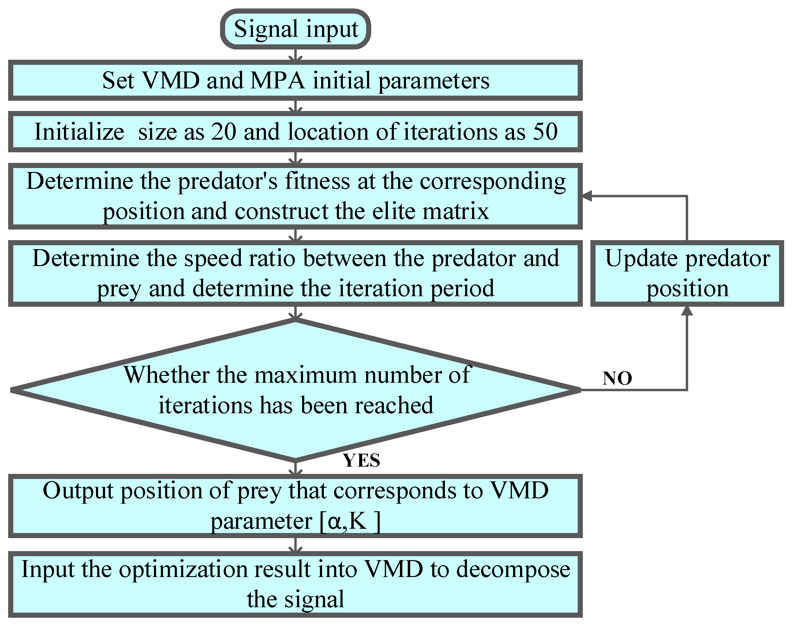
(1)

Set the initial parameters of the VMD and MPA algorithms;

(2)

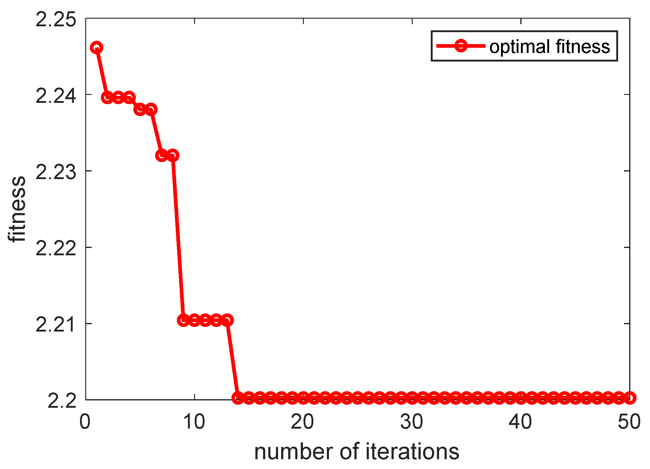
Initialize the number of predator populations and the number of iterations in the MPA algorithm. Considering the influence of population size and number of iterations on optimization accuracy and computational efficiency, this paper defines the population size as 20 and the number of iterations as 50;

(3)

Initialization produces initial prey, and predators build an elite matrix (predator vector). Note that both predators and prey consider themselves search agents because when predators search for prey, the prey is also looking for food. Calculate the fitness value corresponding to that time;

(4)

The MPA optimization process, as described in Section 2.2;

(5)

After updating the predator’s position, the corresponding fitness is calculated and compared to the previous fitness value. Choose the best fitness position as the top predator position;

(6)

Repeat steps (1–5) until the termination condition is met and output the apex predator position coordinates, which are input into the VMD as the optimal parameters for the decomposition signal.

The flowchart of MPA to optimize VMD is given in Figure 1.

It should be noted that in situations where the input dataset exhibits weak correlation, managing the IMF components can be challenging. One approach to addressing this issue is to employ advanced feature selection methods and incorporating domain knowledge can further enhance the management of IMF components in such challenging scenarios. Additionally, one can try to use them in combination with other IMF components that are more correlated. By synthesizing multiple IMF components, the accuracy and stability of the predictive model can be improved.

3. Extreme Learning Machine with Extended Maximum Correntropy Criterion

3.1. Extended Maximum Correntropy Criterion

Correntropy is an effective measure of the generalized similarity between two random variables. Given two random variables $y$, the correntropy can be defined as [23]:

$$V\left(x,y\right)=E\left[{\kappa }_{\sigma }\left(x-y\right)\right]$$

(16)

where ${\kappa }_{\sigma }\left(\cdot \right)$ represents the kernel function with kernel width; $E\left[\cdot \right]$ is the expectation operator. The Gaussian kernel is usually used as a kernel function in (18), expressed as:

$${\kappa }_{\sigma }\left(x-y\right)=G_{\sigma }\left(x-y\right)=\frac{1}{2\pi {\sigma }^2}\exp \left(-\frac{{\left(x-y\right)}^2}{2{\sigma }^2}\right)$$

(17)

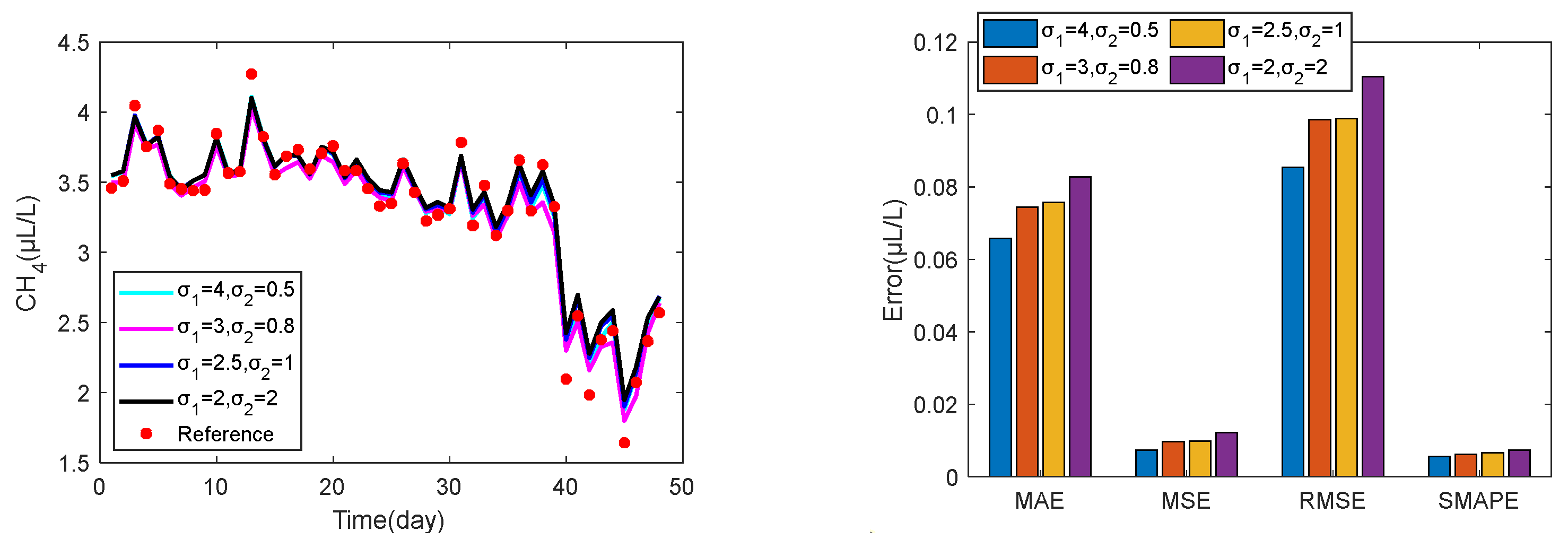
One can see from (17) that the correntropy only contains a second-order moment of error (SOME) with a single kernel width in the exponent part, which may lead to unsuitable performance for complex environments. Therefore, this paper will design a new extended correntropy consisting of two SOME with two different kernel widths in the exponent part, called extended correntropy (ExC), which is defined as:

$$V_C(x,y)=E[{\kappa }_{C,\sigma }(x-y)]$$

(18)

$${\kappa }_{C,\sigma }(x-y)=\exp [-(\gamma \frac{{(x-y)}^2}{2{\sigma }_1^2}+(1-\gamma )\frac{{(x-y)}^2}{2{\sigma }_2^2})]$$

(19)

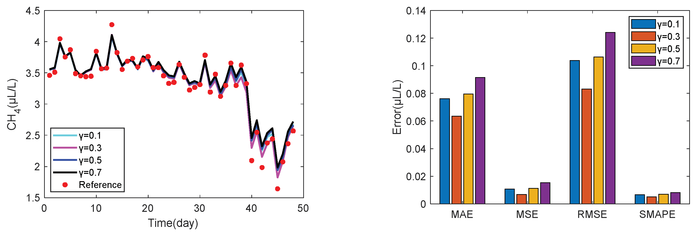
where $\gamma$ is the parameter that determines the ratio of two kernels; ${\sigma }_2$ and ${\sigma }_2$ are different kernel widths, and when ${\sigma }_1={\sigma }_2$ or ($\gamma \to 0(or1)$), the ExC will degenerate to the original correntropy.

In practice, the probability density function of the two random variables is unknown, and the number of samples ${\{x_i,y_i\}}_{i=1}^N$ is finite. Therefore, the sample mean estimate in Equation (20) is defined as:

$$\begin{array}{c}{V}_C^{*}(x,y)=\frac{1}{N}{\displaystyle \sum _{i=1}^N\exp \left[-\left(\gamma \frac{{\left(x_i-y_i\right)}^2}{2{\sigma }_1^2}+(1-\gamma )\frac{{\left(x_i-y_i\right)}^2}{2{\sigma }_2^2}\right)\right]}\\ =\frac{1}{N}{\displaystyle \sum _{i=1}^N{\kappa }_{C,\sigma }}(x_i-y_i)=\frac{1}{N}{\displaystyle \sum _{i=1}^N{\kappa }_{C,\sigma }}(e_i)\end{array}$$

(20)

where N represents the number of samples, $x_i$ and represents the i-th element of random variables $X$ and $Y$.

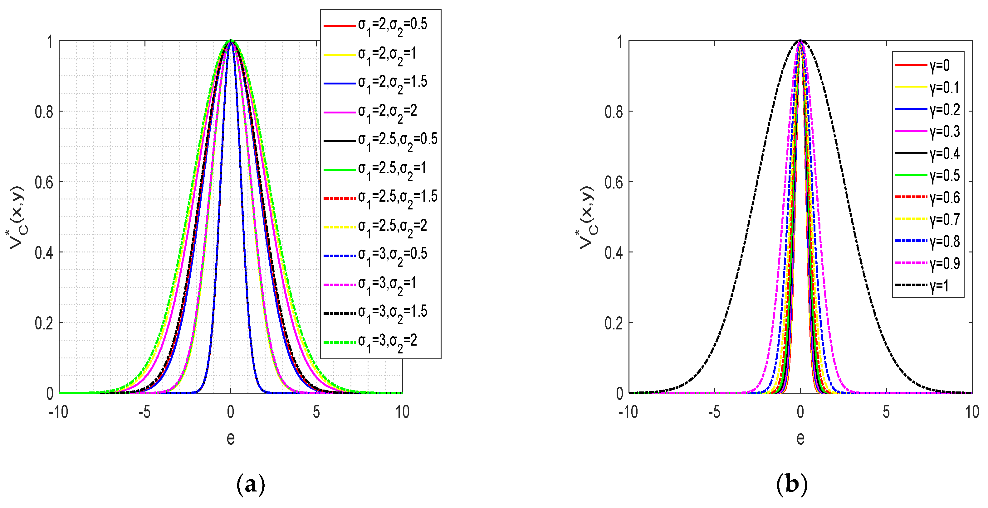
Figure 2 shows the function curve under different parameters, as can be seen from Figure 2a, when y is constant and ${\sigma }_2=0.5$, the curve gradually becomes flat as ${\sigma }_1$ increases. It can be seen from Figure 2b that when the kernel width value is constant, the function curve tends to be flat with the crease of $y$, but the overall trend still meets the requirements of convergence and boundedness.

Finally, in conjunction with Figure 2, we summarize the general properties of ExMCC as follows [30]:

Property 1: Symmetry, $V_C(x,y)=V_C(y,x)$.

Property 2: $V_C(x,y)$ is positive and bounded, $0<V_C(x,y)\le 1$.

Property 3: If $0\le \gamma \le 1$, then $V_C(x,y)$ represents a combined second-order statistic that maps the feature space.

Based on the above properties, we can easily conclude that ExC is an extended form of correntropy. Compared with correntropy, when we select the appropriate free parameters in ExC, it is not only more robust to abnormal data, but also has better convergence speed and stability. Similar to correntropy, the EXC is capable of suppressing the interference of non-Gaussian noise due to its inherent robustness to outliers and its ability to capture higher-order statistical moments beyond the mean and variance. Unlike traditional measures such as the MSE, which are sensitive to outliers and assumptions of Gaussianity, the ExC is based on the probability distribution of the data, allowing it to effectively mitigate the impact of non-Gaussian noise by focusing on the underlying statistical structure of the data rather than solely relying on the second-order statistics. This enables ExC to better capture the true underlying signal in the presence of non-Gaussian noise, making it a valuable tool for robust signal processing. Like the maximum correntropy criterion (MCC), the ExC can also be used as a learning criterion in machine learning fields, which will be denoted as extended MCC (ExMCC) in this work.

3.2. Extreme Learning Machine

An extreme learning machine (ELM) is a single hidden layer feed-forward neural network. The number of hidden layer nodes is usually set artificially, while the input weights and biases are determined randomly. In the process of learning and calculation, the weights and biases are not iteratively calculated, and the optimal solution can be calculated when training data is available. Therefore, compared with traditional feedforward networks such as BP, ELM has more advantages in time series data prediction such as fast training speed, strong generalization ability, fewer hyperparameters, and high accuracy. Recently, ELM has been widely used in the forecasting of time series data, and satisfactory prediction results have been obtained. The calculation procedure of the ELM can be described as follows:

Given a set of sample data $I=\left(x,y\right)$, where $x={\left[x_1,x_2,\dots ,x_N\right]}^T$ and $y={\left[y_1,y_2,\dots ,y_N\right]}^T$ represent N-dimensional input and desired output vectors, respectively. Therefore, the hidden layer output of ELM can be expressed as:

$$\begin{array}{c}h(x_i)=G(w_i,x_i,b_i)\\ \hspace{1em}\hspace{1em}\hspace{1em}\hspace{1em}\hspace{1em}\hspace{1em}=G(w_i{x}_i+b_i)\end{array}$$

(21)

where $h_i(\cdot )$ is the output of the i-th hidden layer node; $w_i$ is the weight between the input layer and the hidden layer; $b_i$ is the hidden layer bias; $G(\cdot )$ is the hidden layer activation function, and in this study, sin is used as the activation function.

Then, we further get the ELM output as:

$$\mathrm{Y}={\displaystyle \sum _{i=1}^L{\beta }_i}{h}_i(x)=\mathrm{H}(x)\mathsf{\beta }$$

(22)

where $\mathrm{Y}={\left[y(x_1),y(x_2),\dots ,y(x_N)\right]}^T$ is the output matrix; $\mathrm{H}(x)={\left[h(x_1),h(x_2),\dots ,h(x_N)\right]}^T,$ $(h(x)={\left[h_1(x),h_2(x),\dots ,h_L(x)\right]}^T)$ is the hidden layer output matrix; $\mathsf{\beta }={\left[{\beta }_1,{\beta }_2,\dots ,{\beta }_N\right]}^T$ is the weight between the output layer and the hidden layer.

By solving the Moore-Penrose generalized inverse matrix of $\mathrm{H}(x)$, and training the ELM by using the input weights and hidden layer bias, the output weights are obtained:

$$\mathsf{\beta }={\mathrm{H}}^{-1}(x)\mathrm{Y}$$

(23)

When employing ELM for time series data forecasting, in certain instances, the weight of the final output of ELM may exhibit significant fluctuations due to substantial changes in forecasted data, consequently leading to poor stability of the forecast results. To address this issue, this paper introduces the ExMCC robust criterion, designed to be impervious to abnormal data, thereby enhancing the robustness of ELM in the presence of abnormal data and effectively mitigating the issue of weight fluctuations caused by abnormal data.

3.3. ELM with ExMCC

In this section, we use ExMCC as a learning criterion for ELM to develop a robust ELM model named ExMCC-ELM, so that when the training data is contaminated, the ELM output can be guaranteed to have a stable optimal weight. The detailed derivation process of ExMCC-ELM is as follows.

Based on the theoretical basis of ExMCC, we rewrite Equation (21) as:

$$\begin{array}{c}\hfill J_C(\beta )=\frac{1}{N}{\displaystyle \sum _{i=1}^N\exp \left[-\left(\gamma \frac{{\left(d_i-h_i{\beta }_i\right)}^2}{2{\sigma }_1^2}+(1-\gamma )\frac{{\left(d_i-h_i{\beta }_i\right)}^2}{2{\sigma }_2^2}\right)\right]}\hfill \\ =\frac{1}{N}{\displaystyle \sum _{i=1}^N{\kappa }_{C,\sigma }}(\mathrm{D}-\mathrm{Y})=\frac{1}{N}{\displaystyle \sum _{i=1}^N{\kappa }_{C,\sigma }}(e_i)\end{array}$$

(24)

where $\mathrm{D}={\left[d_1,d_2,\dots ,d_N\right]}^T$ represents the desired output; $\mathrm{Y}={\left[y(x_1),y(x_2),\dots ,y(x_N)\right]}^T$ represents actual output; $e_i=d_i-y_i=d_i-h_i{\beta }_i$, $d_i,h_i$ and represents the i-th elements of $\mathrm{D},\mathrm{H}$ and $\mathsf{\beta }$.

The optimal solution of the weight $\mathsf{\beta }$ is obtained using the maximization cost function $J_C$. Specifically, $J_C$ finds the differential with respect to the gradient method and makes it zero.

$$\begin{array}{l}\frac{\partial J_{CMC}}{\partial \beta }=0\\ \Rightarrow \frac{1}{N}{\displaystyle \sum _{i=1}^N\left[\exp \left[-\left(\gamma \frac{{\left(d_i-h_i{\beta }_i\right)}^2}{2{\sigma }_1^2}+(1-\gamma )\frac{{\left(d_i-h_i{\beta }_i\right)}^2}{2{\sigma }_2^2}\right)\right]*\left[\frac{\gamma }{{\sigma }_1^2}\left(d_i-h_i{\beta }_i\right)h_i+\frac{1-\gamma }{{\sigma }_2^2}\left(d_i-h_i{\beta }_i\right)h_i\right]\right]}=0\\ \Rightarrow {\displaystyle \sum _{i=1}^N\left[c(e_i)*\left[\left(\frac{\gamma }{{\sigma }_1^2}+\frac{1-\gamma }{{\sigma }_2^2}\right)h_i^T{d}_i-\left(\frac{\gamma }{{\sigma }_1^2}+\frac{1-\gamma }{{\sigma }_2^2}\right)h_i^T{h}_i{\beta }_i\right]\right]}=0\\ \Rightarrow \mathsf{\beta }={\left\{{\displaystyle \sum _{i=1}^N\left[c(e_i)*\left[\left(\frac{\gamma }{{\sigma }_1^2}+\frac{1-\gamma }{{\sigma }_2^2}\right)h_i^T{h}_i\right]\right]}\right\}}^{-1}\left\{{\displaystyle \sum _{i=1}^N\left[c(e_i)*\left[\left(\frac{\gamma }{{\sigma }_1^2}+\frac{1-\gamma }{{\sigma }_2^2}\right)h_i^T{d}_i\right]\right]}\right\}\\ \Rightarrow \mathsf{\beta }={\left[{\mathrm{H}}^T\mathrm{C}\mathrm{H}\right]}^{-1}{\mathrm{H}}^T\mathrm{C}\mathrm{D}\end{array}$$

(25)

$$c(e_i)=\exp \left[-\left(\gamma \frac{{\left(d_i-h_i{\beta }_i\right)}^2}{2{\sigma }_1^2}+(1-\gamma )\frac{{\left(d_i-h_i{\beta }_i\right)}^2}{2{\sigma }_2^2}\right)\right]$$

(26)

where $\mathrm{C}=\mathrm{diag}\left(c(e_i)\right)$ represents the diagonal matrix.

Obviously, Equation (26) is a fixed-point equation $\mathrm{\beta }$, so the fixed-point iterative method is used to calculate the optimal solution for $\mathrm{\beta }$. The overall calculation flow of the proposed ExMCC-ELM algorithm is organized in Algorithm 1. In addition, in ExMCC-ELM, it will degenerate into MC-ELM when $\gamma =0(or1)$ or ${\sigma }_1={\sigma }_2$. Using ExMCC as a learning criterion for ELM can improve ELM robustness by utilizing its ability to model and suppress non-Gaussian noise. Traditional ELM assumes that both input data and noise follow a Gaussian distribution, but in practical applications, non-Gaussian noise such as outliers can often interfere with the data. ExMCC allows for the modeling of non-Gaussian noise. By maximizing the ExC between features and noise, the influence of outliers on the ELM model can be reduced, better adapting to the characteristics of non-Gaussian noise. Therefore, using ExMCC as the learning criterion for ELM can improve ELM robustness in dealing with abnormal data.

Algorithm 1. ExMCC-ELM model. Initialize ExMCC-ELM: ${\sigma }_1,{\sigma }_2,\lambda ,{\beta }_i,b_i$

Training phase:   Training input: $x={\left[x_1,x_2,\dots ,x_{N_1}\right]}^T\Rightarrow (x_i,x_{i+1}),\begin{array}{cc}& 0<i<250\end{array}$   Training output: $y={\left[y_1,y_2,\dots ,y_{N_1}\right]}^T\Rightarrow x_{i+2}$   $\mathrm{Final} \mathrm{output}: \mathsf{\beta },b_i$ Testing phase:   Testing input: $\mathsf{\beta },b_i$ and $x={\left[x_{251},x_{252},\dots ,x_{N_2}\right]}^T\Rightarrow (x_i,x_{i+1}),\begin{array}{cc}& 250<i<300\end{array}$   Testing output: $y={\left[y_1,y_2,\dots ,y_{N_2}\right]}^T\Rightarrow x_{i+2}$   1. For $k\leftarrow 1$ to $M(M=10)$   2. Calculate the error vector $e_i$, based on the initial ${\beta }_i,b_i$: $e_i=d_i-h_i{\beta }_i$   3. Calculate the diagonal matrix $\mathrm{C}$$: \mathbf{C}=\mathrm{diag}\left(c(e_i)\right)$   4. Calculate the output weight $\mathsf{\beta }$$: \mathsf{\beta }={\left[{\mathrm{H}}^T\mathrm{C}\mathrm{H}\right]}^{-1}{\mathrm{H}}^T\mathrm{C}\mathrm{D}$   5. Determine whether the loop ends: $\left|J_C({\mathsf{\beta }}_k)-J_C({\mathsf{\beta }}_{k-1})\right|<\omega ,(\omega =0.00001)$   6. End For

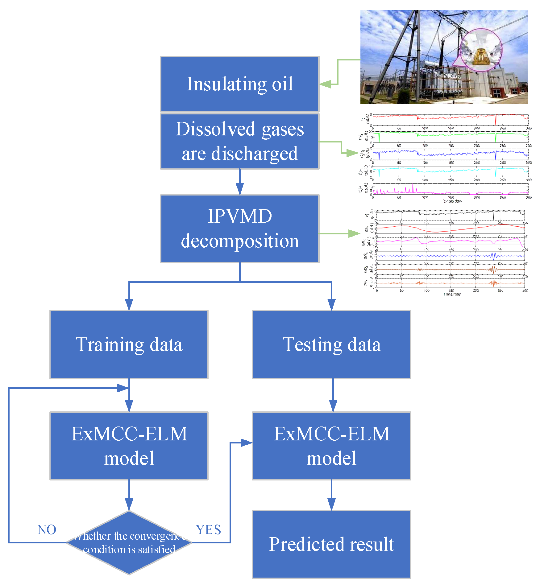
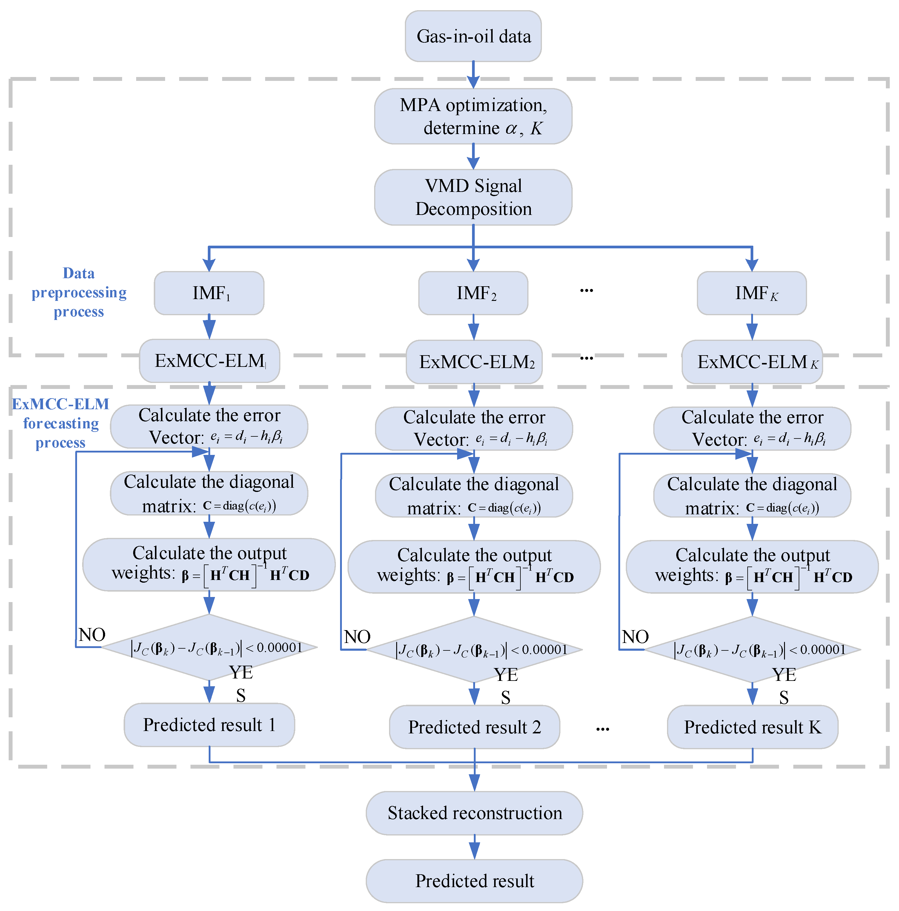
By using the decomposed data obtained from the VMD with MPA optimization developed in Section 2, one can train the proposed model ExMCC-ELM, and then use the test data to evaluate its prediction capability. Figure 3 gives a diagram to illustrate the complete prediction process by using the proposed method for dissolved gases forecasting.

4. Gas-in-Oil Prediction Scheme via ExMCC-ELM and IPVMD

4.1. Data Construction

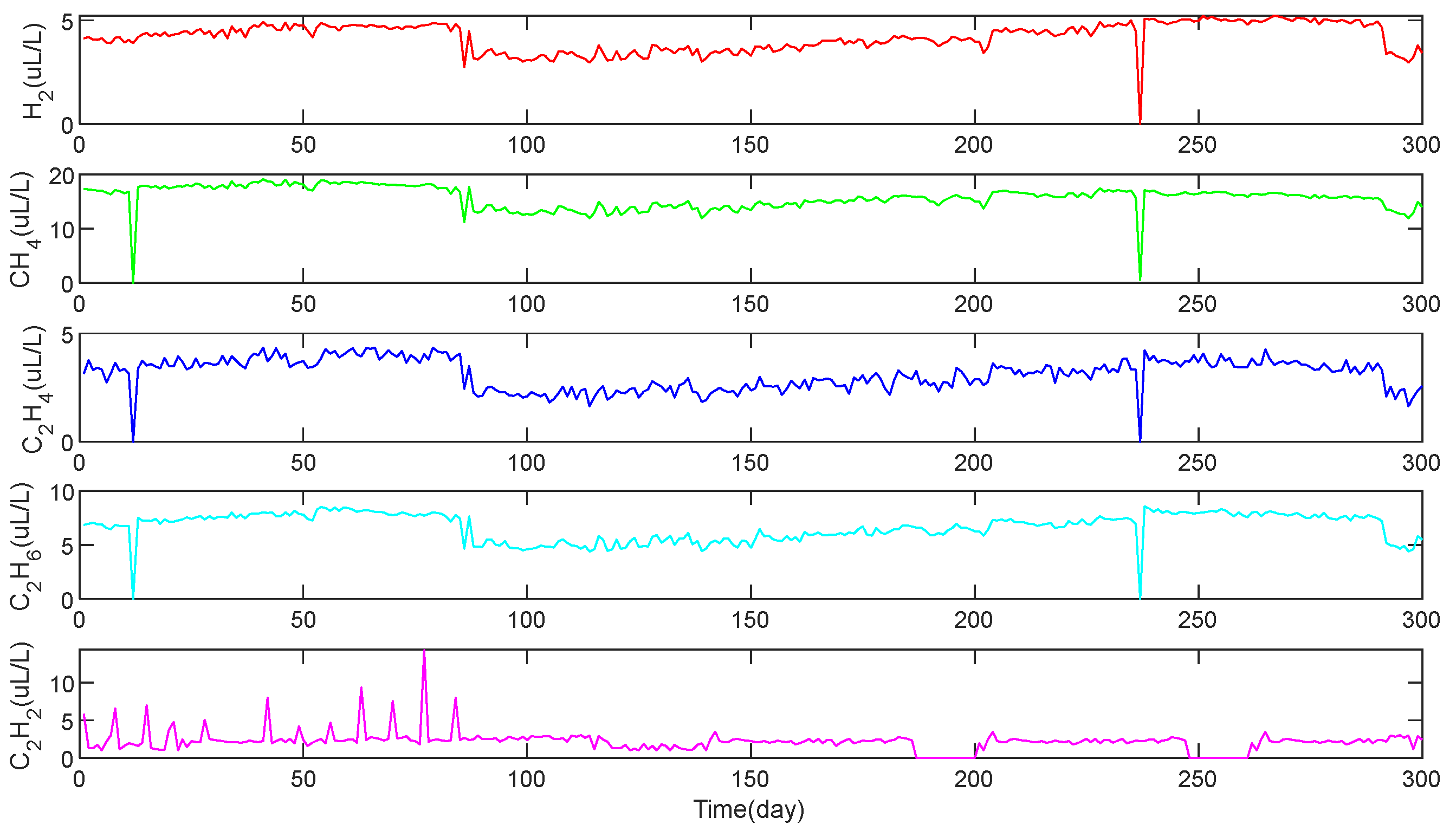
Given the large variety of internal gases in power transformers, the connection between individual gases is not tight and the amount of data is lacking. To solve this problem, this paper uses the method of constructing data pairs to predict various gases.

Firstly, the dissolved gas data in the oil $(H_2,C_2{H}_4,C_2{H}_2,C_2{H}_6,C{H}_4)$ [31] are used as inputs for IPVMD decomposition, and the decomposition vectors of these five gases were obtained respectively.

The raw dissolved gases in oil data are shown in Figure 4.

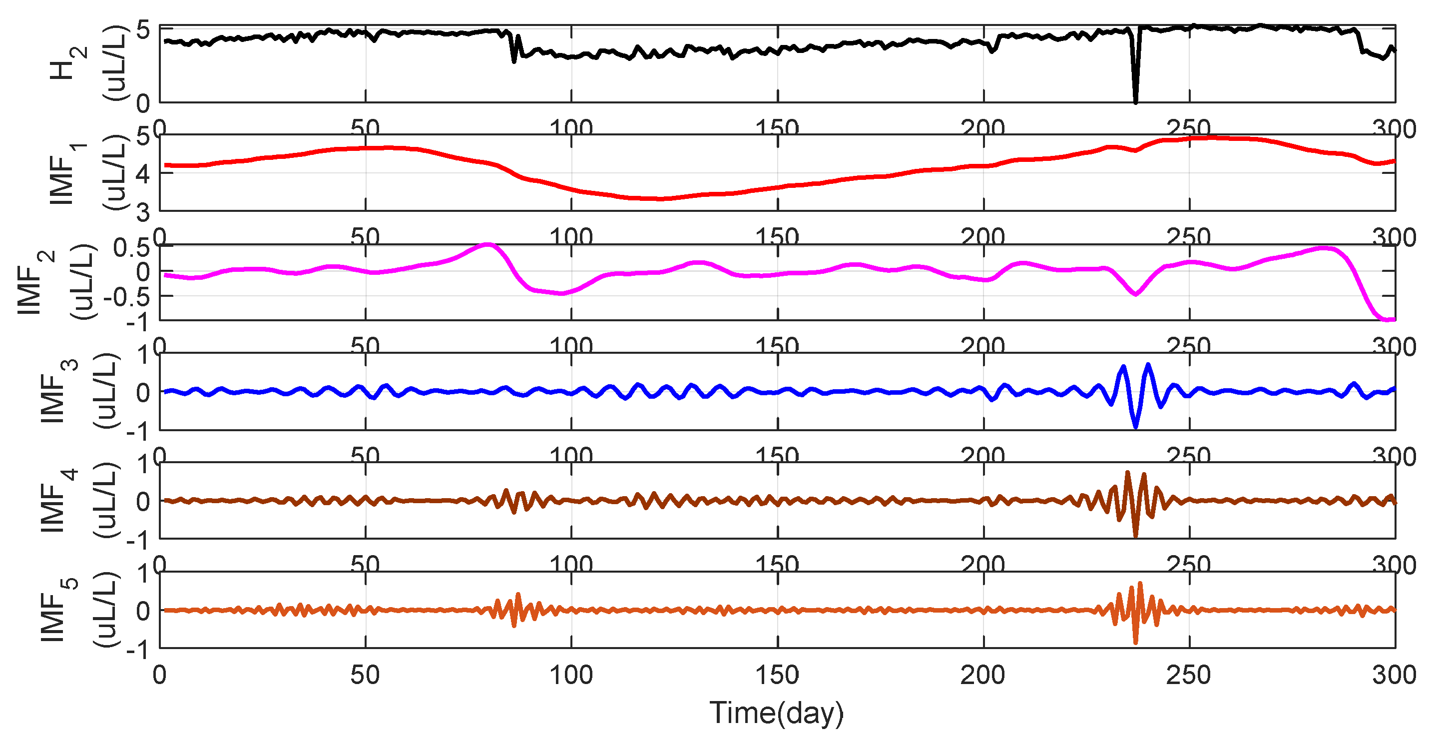
To verify whether IPVMD can efficiently extract the temporal information of the gas content sequence. Taking $H_2$ gas as an example, the IPVMD method was used to perform modal decomposition of the raw $H_2$ data. Figure 5 illustrates the convergence curve of the MPA-optimized VMD decomposition $H_2$ process. Figure 6 shows the raw data of $H_2$ and the five-modal data $\left[{\mathrm{IMF}}_1,{\mathrm{IMF}}_2,\cdots ,{\mathrm{IMF}}_5\right]$ after IPVMD decomposition and the optimized K is selected as 5 by using the MPA algorithm. It can be seen from Figure 5 that the original strong fluctuation and irregular data after VMD decomposition become smooth in the five modes, which is helpful for training and testing the data of each modality.

Then, the limited data sample $IM{F}_k=\left[x_1,x_2,\cdots ,x_{300}\right](k=1:K$), $K$ is the number of modes to be decomposed by the VMD, which is determined by the MPA algorithm) is divided into training data and testing data of the ExMCC-ELM model, respectively, where the first 250 points ${\left\{x_i\right\}}_{i=1}^{250}$ are used as the training set and the last 50 points ${\left\{x_i\right\}}_{i=251}^{300}$ are used as the testing set. Training and testing use data pairs constructed in the form of input and output, respectively.

4.2. MPAVMD-ExMCC-ELM Model Prediction Process

In this paper, the VMD decomposition method is used to decompose the nonstationary timing signal of dissolved gas in transformer oil and convert it into a stationary signal in multi-mode. Secondly, in the face of the uncertainty of signal decomposition, the IO optimization method is further used to optimize the parameters of VMD, and the most satisfactory signal decomposition results have been obtained. Thirdly, the lack of sample data, strong volatility, and poor regularity are not conducive to the characteristics of network model training and testing. This paper introduces ExMCC optimization criteria in the ELM model to overcome the above shortcomings. In this study, the original gas data was divided into training and testing parts, and the

Step 1: Initialize IPVMD and ExMCC-ELM

The exMCC-ELM model was trained with the first 250 sets of data, the last 50 sets of data were tested, and the gas data involved was included $H_2,C_2{H}_4,C_2{H}_2,C_2{H}_6,C{H}_4$.

The specific steps are as follows:

Step 2: The gas data $H_2,C_2{H}_4,C_2{H}_2,C_2{H}_6,C{H}_4$ was decomposed by IPVMD respectively to obtain its decomposition vector $\left[{\mathrm{IMF}}_1,{\mathrm{IMF}}_2,\cdots ,{\mathrm{IMF}}_K\right]$. $K$ is the number of modes of VMD decomposition, which is determined by the VMD optimization algorithm, and the $K$ value may be different for different gases.

Step 3: The obtained decomposition vector $IM{F}_k=\left[x_1,x_2,\cdots ,x_{300}\right]$$(k=1:K)$ is used as the training data and test data of the ExMCC-ELM model respectively, where the first 250 points are used as the training set and the last 50 points are used as the test set. Training and testing use data pairs constructed in the form of input and output, respectively. That is, the input and output of the ExMCC-ELM model training process are: $x={\left[x_1,x_2,\dots ,x_{N_1}\right]}^T\Rightarrow (x_i,x_{i+1}),\begin{array}{cc}& 0<i<250\end{array}$, $y={\left[y_1,y_2,\dots ,y_{N_1}\right]}^T\Rightarrow x_{i+2}$; The input and output of the test process are $x={\left[x_{251},x_{252},\dots ,x_{N_2}\right]}^T\Rightarrow (x_i,x_{i+1}),\begin{array}{cc}& 250<i<300\end{array}$, $y_k={\left[y_1,y_2,\dots ,y_{N_2}\right]}^T\Rightarrow x_{i+2}$.

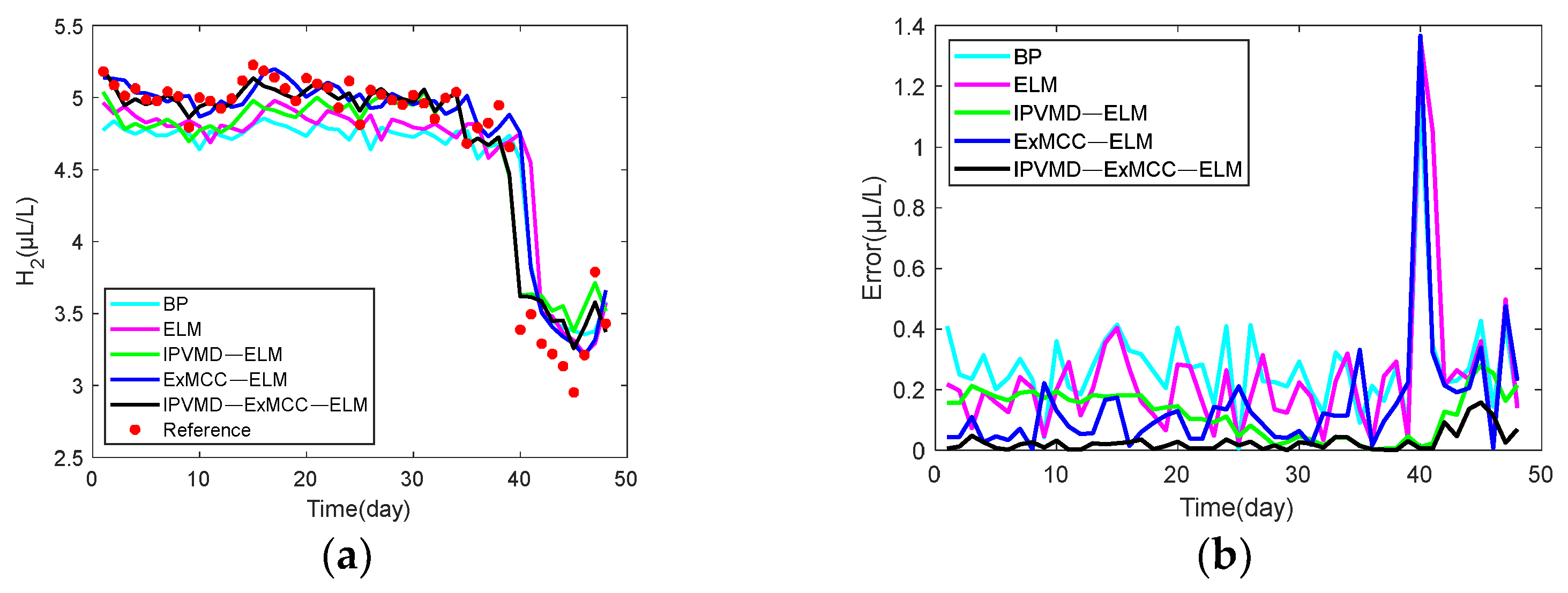
Step 4: The prediction results of each decomposition vector $\left[{\mathrm{IMF}}_1,{\mathrm{IMF}}_2,\cdots ,{\mathrm{IMF}}_K\right]$ are reconstructed to obtain the prediction results of the raw gas: $y=\frac{1}{K}{\displaystyle \sum _{k=1}^K{y}_k}$.

In this paper, the performance of the prediction method is evaluated using mean absolute error (MAE), mean squared error (MSE), root mean square error (RMSE), and symmetric mean absolute percentage error (SMAPE), defined as follows:

$$\begin{array}{c}MAE=\frac{1}{N}{\displaystyle \sum _{i=1}^N|}{d}_i-y_i|\\ MSE=\frac{1}{N}{\displaystyle \sum _{i=1}^N{\left(d_i-y_i\right)}^2}\\ RMSE=\sqrt{\frac{1}{N}{\displaystyle \sum _{i=1}^N{\left(d_i-y_i\right)}^2}}\\ SMAPE=\frac{100\%}{N}{\displaystyle \sum _{i=1}^N\frac{\left|d_i-y_i\right|}{\left(\left|d_i\right|+\left|y_i\right|\right)/2}}\\ \end{array}$$

(27)

where $N$ is the sample size; $d_i$ is the expected value; $y_i$ is the actual predicted value.

The structure diagram of the IPVMD-ExMCC-ELM model for predicting dissolved gases in transformer oil can be seen in Figure 7.

5. Experiments and Analysis

In this study, BP, ELM, IPVMD-ELM, and ExMCC-ELM were used as the control experimental groups to reflect the performance of the proposed method under various test conditions. All simulations in this paper are performed using MATLAB 2022a in i5-8250 U and 1.6 GHz CPUs.

5.1. Prediction and Analysis of $H_2$

To verify whether IPVMD can effectively extract the time information of the gas content sequence. In this section, taking $H_2$ gas as an example, the original $H_2$ data were decomposed using the IPVMD method, and then tested and verified based on ELM and the improved ExMCC-ELM model.

To demonstrate the effectiveness and rationality of the experiment, we use BP, ELM, and ExMCC-ELM as comparative tests to verify the effectiveness of the proposed method based on the gas data in the original state. In this paper, BP is set to the single hidden layer, the number of neurons in the hidden layer is set to 10, and the number of neurons in the hidden layer of ELM, IPVMD-ELM, ExMCC-ELM, and IPVMD-ExMCC-ELM is set to 5, 5, 3, and 3, respectively, to ensure that each method is in the best prediction state. Figure 8 shows the prediction results and errors of various methods for 50-day $H_2$ data, as shown in the figure, the prediction results based on the original $H_2$ data have a large error, compared with BP and ELM models, the ELM model based on ExMCC optimization criterion improves the prediction results to a certain extent, because the ExMCC criterion is not sensitive to strongly fluctuating data, indicating that ExMCC is effective for the improvement of ELM model. However, this improvement did not allow the ExMCC-ELM model to maintain its intended performance throughout the process. This suggests serious drawbacks to directly applying raw $H_2$ data for the next time series forecast. However, based on the $H_2$ data after IPVMD modal decomposition, this problem can be effectively solved, and the decomposed data can effectively solve the influence of data mutation on the original ELM model, which greatly improves the prediction accuracy.

It can be seen from the data in

Table 1. $H_2$ prediction results for each method.

	BP	ELM	IPVMD-ELM	ExMCC-ELM	IPVMD-ExMCC-ELM
MAE	0.2741	0.2350	0.1595	0.1485	0.0863
MSE	0.1027	0.1082	0.0361	0.0633	0.0147
RMSE	0.3204	0.3289	0.1900	0.2517	0.1211
SMAPE	0.0153	0.0133	0.0092	0.0087	0.0053

that the MAE and MSE results of IPVMD-ELM are 32.13% and 66.64% lower than those of ELM prediction results, respectively, and the IPVMD-ELM prediction error is relatively stable and there is no huge mutation. The IPVMD-ExMCC-ELM model synthesizes all the characteristics of IPVMD and ExMCC optimization criteria, showing excellent robustness, estimation accuracy, and stability.

5.2. Prediction and Analysis of Other Gases

After the detailed analysis in the previous section, we have obtained the optimal performance of the IPVMD-ExMCC-ELM method in decomposing and predicting the original $H_2$ gas. However, in power transformer oil, there are usually multiple hydrocarbon gases present, such as ${\mathrm{CH}}_4$, ${\mathrm{C}}_2{\mathrm{H}}_2$, ${\mathrm{C}}_2{\mathrm{H}}_4$, and ${\mathrm{C}}_2{\mathrm{H}}_6$, with weak correlations among them. This weak correlation makes it challenging to estimate the individual gas concentrations jointly. Therefore, further validation is needed to assess the applicability of the proposed method for predicting different gas data. Figure 9, Figure 10, Figure 11 and Figure 12 demonstrate the prediction results and errors for several different gases.

Table 2. Prediction results evaluation for each method.

		BP	ELM	IPVMD-ELM	ExMCC-ELM	IPVMD-ExMCC-ELM
${\mathrm{CH}}_4$	MAE	0.4056	0.3244	0.1833	0.2747	0.1135
	MSE	0.2721	0.2432	0.0457	0.1798	0.0255
	RMSE	0.5217	0.4931	0.2137	0.4240	0.1597
	SMAPE	0.0067	0.0054	0.0029	0.0046	0.0019
${\mathrm{C}}_2{\mathrm{H}}_2$	MAE	0.4143	0.3846	0.1807	0.3994	0.1196
	MSE	0.2647	0.2554	0.0501	0.2184	0.0263
	RMSE	0.5145	0.5054	0.2239	0.4673	0.1620
	SMAPE	0.1315	0.1374	0.1118	0.1310	0.1028
${\mathrm{C}}_2{\mathrm{H}}_4$	MAE	0.2738	0.2480	0.0921	0.2284	0.0670
	MSE	0.1453	0.1316	0.0149	0.1148	0.0073
	RMSE	0.3811	0.3628	0.1222	0.3389	0.0855
	SMAPE	0.0221	0.0203	0.0080	0.0184	0.0056
${\mathrm{C}}_2{\mathrm{H}}_6$	MAE	0.3027	0.2952	0.1682	0.2586	0.1044
	MSE	0.1984	0.2036	0.0675	0.1638	0.0209
	RMSE	0.4455	0.4513	0.2599	0.4047	0.1445
	SMAPE	0.0117	0.0111	0.0069	0.0096	0.0042

lists the evaluation indicators for each prediction result, and the data in the table shows that the proposed methods exhibit good predictive performance compared to the IPVMD-ExMCC model, which has higher accuracy. In ${\mathrm{C}}_2{\mathrm{H}}_4$ with the highest prediction accuracy, MAE, MSE, and SMAPE were improved by 27.25%, 51.01%, and 30.00%, respectively. In ${\mathrm{CH}}_4$ with lower prediction accuracy, MAE, MSE, and SMAPE were improved by 38.08%, 44.20%, and 34.48%, respectively. It can be seen that the proposed IPVMD-ExMCC-ELM model can accurately predict the content of dissolved gas in power transformer oil.

5.3. Analysis of the Impact of Different Parameter Settings on the Prediction Effect

In this section, we will investigate the influence of kernel width $\sigma$ and scale factor $\gamma$ on the proposed IPVMD-ExMCC-ELM model. As shown in Figure 13, when the scale factor is fixed, the prediction accuracy of the model is weakly affected by different kernel widths. In contrast, the estimation error obtained when ${\sigma }_1={\sigma }_2$ is the largest, which fully indicates that the proposed ExMCC optimization criterion is better than the original MC. Figure 14 shows that when the core width is fixed, the prediction error increases as the $\gamma$ increases. This is because a small kernel width is conducive to suppressing the effects of abnormal data or large fluctuations, and this suppression effect gradually decreases as the core width increases. Therefore, the estimation error gradually increases. After the simulation study in this paper, the entropy gravity with a small kernel width should dominate the ExMCC in all experiments, and the predicted effect of the proposed method is the best when ${\sigma }_1=4,{\sigma }_2=0.5,$ and $\gamma =0.3$.

6. Conclusions

The power transformer is an important bridge for energy transmission and conversion in the power system, which is of great significance to the safe operation of the system. To realize the prediction of gas in transformer oil, a new IPVMD-ExMCC-ELM prediction model is proposed. Firstly, the IPVMD decomposition method is used to perform modal decomposition of the original gas dataset to obtain a stable data set that is easy to process. Then, the application of ELM in the prediction of dissolved gas concentration in transformer oil is introduced, and the proposed ExMCC optimization criterion is introduced into ELM. The simulation results show that the robust prediction method based on IPVMD-ExMCC-ELM proposed in this paper can accurately predict gas content under the condition of uncertain gas content mutation and oscillation law. The effectiveness and feasibility of the proposed method are verified by simulation analysis. In general, the advantages of IPVMD-ExMCC-ELM proposed in this paper are mainly reflected in the following aspects: Under the evaluation indexes of MAE, MSE, RMSE, and SMAPE, IPVMD-ELM and ExMCC-ELM have higher prediction accuracy than traditional ELM. On the other hand, IPVMD-ExMCC-ELM has higher predictive accuracy than IPVMD-ELM and ExMCC-ELM.