Research on Diesel Engine Speed Control Based on Improved Salp Algorithm

Abstract

To better regulate the speed of diesel engines and optimize the speed overshoot and fast response, a speed control method combining the improved salp swarm algorithm (ISSA) with the proportional integral and differential (PID) controller was proposed. A real-time simulation model for a high-pressure common rail diesel engine was established. Addressing the challenges of the salp swarm algorithm (SSA), such as uneven population distribution and its tendency to become trapped in local optima, logistic-tent chaotic mapping, adaptive parameters was introduced, as well as adaptive dynamic inertia weights, elite strategy, and a dynamic inverse strategy. These enhancements bolstered the algorithm’s precision and efficiency in both global and local searches. Using the enhanced SSA, the parameters of the PID controller for the diesel engine model was optimized. The results indicated that the ISSA offers superior parameter identification precision, strengthening speed control stability. During sudden changes in speed and load, the overshoot decreased by an average of more than 30.3% and more than 8.6%, respectively. Moreover, the settling time decreased by an average of more than 0.76 s and 1.52 s, respectively, significantly enhancing the quality of diesel engine speed control.

1. Introduction

The rotational speed of diesel engines profoundly influences critical parameters, such as combustion processes, power output, and energy efficiency. Thus, controlling the speed of a diesel engine plays a pivotal role in determining the performance and stability of diesel automotive power systems. In diesel engines, speed control is essential to ensure the combustion process’s efficacy. Proper speed control refines the combustion process, enhances combustion efficiency, and curtails pollutant emissions. Additionally, controlling the engine’s speed directly determines the strength and consistency of its power output. By meticulously modulating the speed, power output demands under diverse load conditions can be met, leading to a more seamless and dependable driving experience. Moreover, controlling a diesel engine’s speed significantly influences its energy efficiency. Appropriate speed modulation, while maintaining power output, reduces fuel consumption and maximizes fuel utilization, elevating the diesel engine’s energy efficiency. This process not only slashes operational costs and minimizes energy consumption but also alleviates environmental strain. Currently, the PID control algorithm is a predominant method for controlling diesel engine speed. This algorithm boasts numerous merits, such as its foundational simplicity, robust adjustability, and ease of implementation [1,2,3]. However, PID can be sensitive to parameter tweaks and might exhibit weaker control over nonlinear systems. The complex, nonlinear journey from fuel injection and combustion work to driving torque output demands traditional control strategies to calibrate numerous maps [4], only allowing for offline tuning without online adjustments. Further, choosing and tweaking the parameters of the PID control algorithm demand a depth of expertise and experience [5,6,7].

In recent years, many researchers have begun to harness the capabilities of artificial intelligence to optimize both the parameters and the architecture of PID [8,9,10,11,12]. Such applications enable the PID controllers to cater to the intricate control requirements of nonlinear, time-variant, and uncertain systems, thereby enhancing the system’s adaptability and robustness. Currently, the prevalent types of intelligent PID controllers include fuzzy PID [13,14], neural network PID [15,16], and expert system-based PID controllers [17,18]. All of these controllers demonstrate commendable control outcomes when tailored to specific practical application demands. In terms of speed control optimization, a study [19] pioneered the application of fuzzy control to diesel engine speed regulation, granting the speed control system elevated robustness and responsiveness. Another study [20] introduced a speed anti-disturbance control algorithm based on parameter self-learning, which swiftly compensated for loads to augment the speed’s anti-disturbance ability. However, the research was confined to a single set speed, with substantial fluctuations at other speeds. A study [21] employed a strategy based on model reference adaptive control (MRAC) that expands upon the discrete-time minimum control synthesize integration (DTMCSI) algorithm, allowing for rapid dynamic tracking of the diesel engine speed and achieving closed-loop control stability. Swarm intelligence algorithms have been continuously evolving, presenting a novel perspective and methodology for addressing intricate challenges, subsequently establishing themselves as an essential branch in overcoming complex optimization problems. In essence, PID parameter tuning is an intricate optimization problem in which ideal parameters are sought to achieve optimized control. Thus, swarm intelligence algorithms are exceptionally apt for addressing such challenges [22,23].

The SSA is a novel swarm intelligence algorithm characterized by fewer parameters, a simple structure, and ease of implementation. Compared to the genetic algorithm and particle swarm optimization, the SSA offers a more streamlined structure while ensuring optimization accuracy, making it suitable for controller applications and producing effective control outcomes. Relative to traditional PID control, using the SSA for PID tuning results in enhanced speed stability and quicker response times. This outcome not only reduces the cost associated with parameter calibration but also elevates the development efficiency of the electronic control unit (ECU). However, the SSA is prone to becoming trapped in local optima. This paper introduces an enhanced SSA to optimize the PID controller parameters of a diesel engine speed control system. Focusing on the high-pressure common rail diesel engine, the research addresses speed fluctuations and overshoot under varying conditions. By leveraging chaos theory, the algorithm enhances population diversity. Adaptive parameters extend the search scope, and adaptive dynamic inertia weights, combined with elite strategies, optimize global search capabilities. Dynamic inversion strategies are incorporated to overcome local optima, facilitating the tuning of PID controller parameters. MATLAB/Simulink simulation results demonstrate that this approach offers reduced steady-state errors, swift responses, and minimal overshoot, leading to an improvement in the quality of diesel engine speed control.

The remaining sections are organized as follows. Section 2 outlines the construction of the diesel engine model. Section 3 delves into the foundational theory of the SSA and its enhancement measures and validates the performance of the ISSA. Section 4 employs data analysis to corroborate the reliability of the proposed approach. Finally, Section 5 concludes the story.

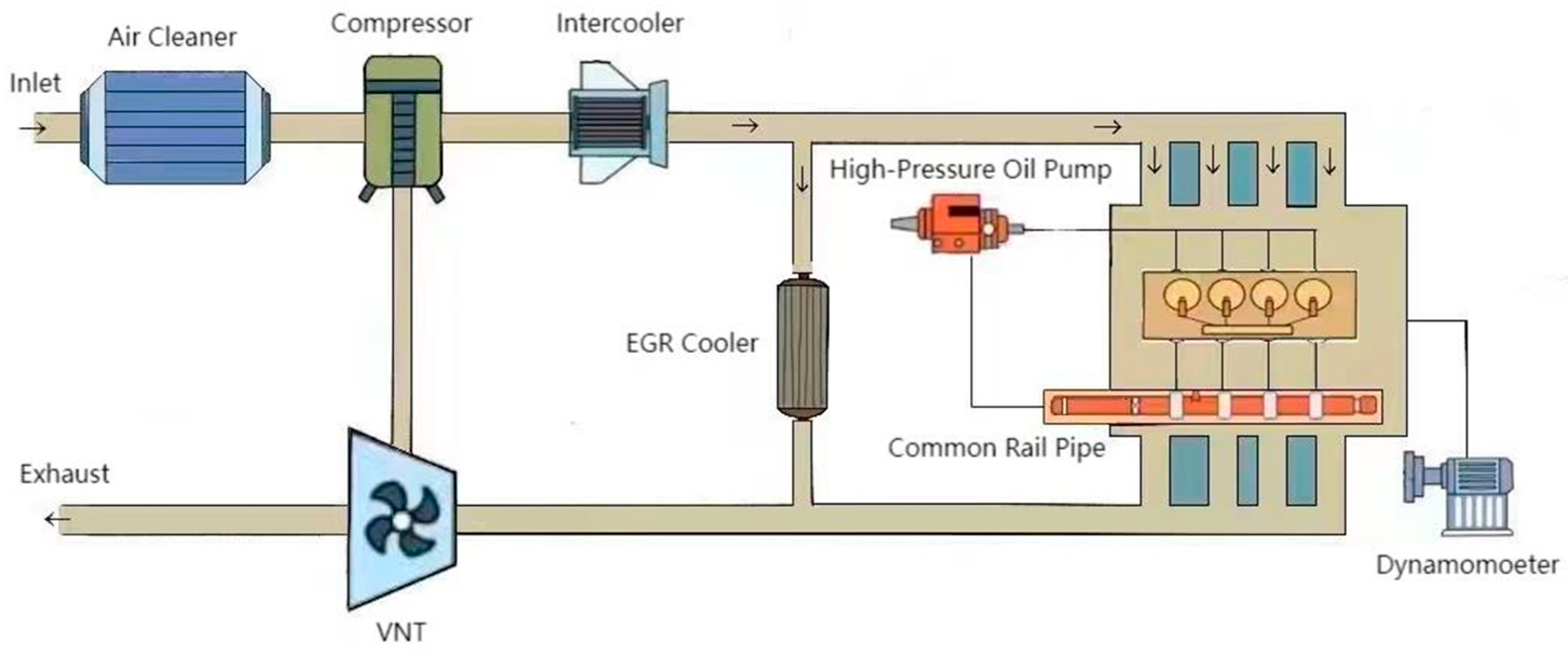
2. Diesel Engine System Model

The study focuses on a turbocharged, intercooled, four-cylinder, high-pressure common rail diesel engine as the controlled object. Upon engine start-up, fuel is pumped from the fuel tank and delivered to the injectors via a fuel pump. The intake system draws fresh air, which, after passing through a compressor, is directed to the intercooler for cooling. The cooled air is further compressed in the intake manifold before entering the cylinders. Fuel and air mix in the combustion chamber and are ignited post-injection by the injectors. The energy produced from combustion propels the piston downward, driving the connecting rod and crankshaft, thus powering the engine. The cooling system employs a circulating coolant to absorb and dissipate the engine’s heat, ensuring its temperature remains within an appropriate range.

Using CRUISE M, a diesel engine model based on physical principles and experimental data is constructed. The model encompasses components such as the air filter, turbocharger, high-pressure common rail, intercooler, and exhaust gas recirculation system. The primary engine parameters are presented in

Table 1. Main Parameters of the Diesel Engine.

Parameter	Numerical Value
Type	Supercharged Intercooled In-Line 4 Cylinders
Cylinder Bore	95 mm
Stroke	105 mm
Rated Power	130/(3200 r/min)kW
Compression Ratio	17.5
Displacement	2.977 L

[24,25].

The framework of the diesel engine model, constructed using Cruise M, is depicted in Figure 1.

2.1. Air Cleaner

The air filter model simulates the flow rate and pressure drop between turbocharging chambers. Through modeling of the mass flow rate of the air filter, the flow from the stagnation conditions in the upstream storage components to the downstream storage components via orifices and adjacent pipes is accounted for.

2.1.1. Flow Exchange Model

Heat exchangers and the exhaust aftertreatment devices are modeled using a simple orifice equation:

$$\stackrel{·}{m}=\mu A_{geom}{p}_{up}\sqrt{\frac{2}{R_{up}{T}_{up}}}\cdot \psi$$

(1)

Herein, $\stackrel{·}{m}$ represents the mass flow rate, $\mu$ denotes the dynamic viscosity, $A_{geom}$ stands for the orifice area, $p_{up}$ is the upstream pressure, $R_{up}$ signifies the upstream specific gas constant, $T_{up}$ indicates the upstream flow temperature, and $\psi$ corresponds to the flow function.

2.1.2. Pressure Drop Model

The pressure drop model can generally be determined based on the wall friction coefficient:

$$\Delta p=F_{fr}\cdot \zeta \cdot \frac{L}{D_{hyd}}\cdot \frac{\rho \cdot {\upsilon }^2}{2}$$

(2)

In the formula, $L$ represents the length of the component after the hole, $D_{hyd}$ denotes the diameter after the hole, $\rho$ stands for the density of the gas, $\zeta$ is determined by the Reynolds number $Re$ and changes based on the flow conditions:

• Laminar flow: $Re=R{e}_l=2300|\zeta ={\zeta }_1$
• Transition flow: $R{e}_l=2300<Re<R{e}_t=5600$
  $\zeta ={\zeta }_1\cdot \left(1-\frac{Re-R{e}_1}{R{e}_t-R{e}_1}\right)+{\zeta }_t\cdot \left(\frac{Re-R{e}_1}{R{e}_t-R{e}_1}\right)$
• Turbulent flow: $Re\ge R{e}_l=5600|\zeta ={\zeta }_t$

In the laminar flow region, the Hagen–Poiseuille law describes laminar pipe flow, where the friction coefficient is calculated as follows:

$${\zeta }_1=\frac{a}{Re}$$

(3)

In the equation, $a$ represents the laminar friction coefficient, which, according to the Hagen–Poiseuille law, is set to 64.

The friction coefficient in turbulent flow, ${\zeta }_t$ is calculated as follows:

$${\zeta }_t=4\cdot (A+B\cdot R{e}^{-1/m})$$

(4)

In the formula, the coefficient $A$, multiplier $B$, and exponent $m$ are derived from reference [26]. Within the model, a multiplier value of 1 is set.

2.2. Turbocharger Model

The turbocharger is a device that integrates a compressor, a turbine, and an intermediate shaft. The turbine is driven by exhaust gases, and the compressor is mechanically connected to the turbine and is rotated by it. The parameters in its characteristic curve, such as isentropic efficiency, the boost ratio, the expansion ratio, and flow rate relationships, are measured under standard experimental conditions. To ensure accuracy when environmental conditions change, corrections to the rotational speed and mass flow rate are required. The correction formula is as follows:

$$n_{cor}=\frac{n_0}{\sqrt{T_1}}$$

(5)

$${\stackrel{·}{m}}_{cor}=\frac{\stackrel{·}{m_c}\cdot \sqrt{T_1}}{p_1}$$

(6)

In the equation, $n_{cor}$ represents the corrected rotational speed of the turbocharger; $n_0$ is the current rotational speed; $T_1$ is the reference temperature obtained from experiments; ${\stackrel{·}{m}}_{cor}$ denotes the corrected mass flow rate of the turbocharger; ${\stackrel{·}{m}}_c$ is the current mass flow rate; and $p_1$ is the pressure as measured in experiments.

2.3. Exhaust Gas Turbocharger Recirculation Model

The exhaust gas recirculation (EGR) model primarily functions for cooling and pressure reduction. The pressure drop of the exhaust passing through the EGR valve is determined by the orifice flow equation, which is calculated as follows:

$$p_1^{*}-p_2^{*}=\frac{\stackrel{·}{m^2}}{2\cdot \rho \cdot A^2\cdot {\mu }^2}$$

(7)

In the formula, $p_1^{*}$ represents the inlet pressure of the EGR; $p_2^{*}$ denotes the outlet pressure of the EGR; $\rho$ stands for the density of the mixed gas; $A$ is the cross-sectional area of the valve; and $\mu$ is the flow coefficient.

After passing through the EGR valve, the gas is cooled by the EGR cooler. The relationship between the inlet and outlet temperatures is as follows:

$$T_1^{*}=T_2^{*}+{\eta }_e(T_1^{*}-T_l)$$

(8)

In the equation, $T_1^{*}$ represents the inlet temperature; $T_2^{*}$ denotes the outlet temperature; ${\eta }_e$ stands for the cooling efficiency; and $T_l$ is the temperature of the cooling fluid.

The EGR rate of the model is calculated as follows:

$$T_e=f_{ex}/(f_i+f_{ex})$$

(9)

In the equation, $T_e$ represents the EGR rate; $f_i$ denotes the intake air flow rate; and $f_{ex}$ stands for the exhaust gas flow rate.

2.4. High-Pressure Common Rail System Model

The fuel injection curve, determined by the crankshaft angle obtained from experiments, serves as the input for the diesel engine combustion simulation. A real-time simulation model of the common rail injection system is established for rapid computation. The injection process is calculated based on the decomposition of the crankshaft angle.

2.4.1. Common Rail Model

The rail is modeled as a 0D pressure-ventilation system, considering the compressibility of the liquid working fluid. In this context, the pressure under isothermal flow is computed using the continuity equation. The volumetric modulus $E$ of the working fluid is derived from the inherent fluid properties database in CRUISE M. The rail pressure is calculated based on the following formula:

$$\frac{d{p}_{rail}}{dt}=\frac{E}{V_{rail}}\cdot \frac{1}{p_{rail}}\cdot (\frac{d{m}_{pump}}{dt}+\frac{d{m}_{inj}}{dt})$$

(10)

In the formula, $p_{rail}$ represents the internal pressure of the common rail; $t$ denotes time; $E$ stands for the volumetric modulus of the working fluid; $V_{rail}$ is the volume of the rail; ${\rho }_{rail}$ indicates the density of the fluid within the rail; $\frac{d{m}_{pump}}{dt}$ is the mass flow rate through the pump; $\frac{d{m}_{inj}}{dt}$ signifies the mass flow rate through the injector.

2.4.2. Fuel Injector Model

The injection rate is calculated based on the nozzle orifice area and injection velocity. The velocity is determined using the viscous flow Bernoulli equation, with the resulting formula accounting for fuel density and the discharge coefficient. This discharge coefficient represents frictional losses throughout the injection system, spanning from the pipeline pressure measurement location to the flow in the injector pipe and the orifices of the injector nozzle. The characteristics of the discharge coefficient are measured as a function of the needle lift on the injector test bench. The incompressible orifice flow formula is as follows:

$${\stackrel{·}{m}}_{fuel}=A_{NH}\cdot c_D\cdot \sqrt{2\cdot {\rho }_{fuel}\cdot (p_{pipe}-p_{cyl})}$$

(11)

In the formula, ${\stackrel{·}{m}}_{fuel}$ represents the fuel injection mass flow rate; $A_{NH}$ denotes the nozzle orifice area; $c_D$ is the discharge coefficient; ${\rho }_{fuel}$ indicates the fuel density; $p_{pipe}$ stands for the pressure inside the pipe; and $p_{cyl}$ signifies the pressure within the cylinder.

The engine speed is given by the following equation:

$$n_{{}_{cng}}=\frac{30\cdot i_s}{m_{cyc}}\cdot \frac{dm}{dt}$$

(12)

In the equation, $i_s$ represents the type of stroke; $m_{cyc}$ denotes the injection mass per cycle; and $\frac{dm}{dt}$ is the mass flow rate of injection per second.

2.4.3. Pressure Pulsation Model

In the simplified model analogy, the interaction between the inert fluid mass in the pipeline and the compressible fluid volume in the rail can be likened to a spring–mass–damper system. Assuming that the length of the system is much greater than its diameter, this system allows for $dV/V=dl/l$. Furthermore, the resonant frequency of pressure pulsations can be approximated as:

$$f=\frac{1}{2\pi }\cdot \sqrt{\frac{c}{m}}=\frac{1}{2\pi }\cdot \sqrt{\frac{E}{l_{pipe}{}^2\cdot {\rho }_{fuel}}}$$

(13)

In the equation, $f$ represents the resonant frequency; $E$ denotes the volumetric modulus of the working fluid; $l_{pipe}$ is the length of the pipeline; and ${\rho }_{fuel}$ indicates the fuel density.

3. Control Algorithm Design

The salp is a type of marine invertebrate. The SSA draws inspiration from the gregarious behavior of salps. The population is divided into two groups: leaders and followers. The leader is the salp at the forefront of the chain, while the remaining salps are considered followers. The leader guides the group, and the followers either directly or indirectly follow one another [27].

3.1. Leader Position

3.1.1. Salp Swarm Algorithm

During the iterative computation of the algorithm, the food source represents the position of the individual with the best fitness. The leader in the population explores the space through random walks. The leader updates its position using the following formula:

$$X_j^1=\{\begin{array}{c}{F}_j+c_1\left(\left(u{b}_j-l{b}_j\right)c_2+l{b}_j\right)\begin{array}{cc}& c_3\ge 0\end{array}\\ F_J-c_1\left(\left(u{b}_j-l{b}_j\right)c_2+l{b}_j\right)\begin{array}{cc}& c_3<0\end{array}\end{array}$$

(14)

$$c_1=2e^{-{\left(\frac{4L}{L_{\max }}\right)}^2}$$

(15)

where, $X_j^1$ represents the position of the first salp in dimension $j$, and $F_j$ denotes the position of the food source in dimension $j$. $u{b}_j$ indicates the upper limit of dimension $j$, while $l{b}_j$ represents the lower limit. $L$ represents the current iteration count, and $L_{\max }$ denotes the maximum number of iterations. $c_2$ and $c_3$ are random numbers between 0 and 1, determining the next position in dimension $j$.

3.1.2. Follower Position

The algorithm employs the delayed motion of the followers to discover more optimal positions. The follower’s position is derived from Newton’s laws of motion:

$$X_j^i=\frac{1}{2}a{t}^2+v_{0}t$$

(16)

where $X_j^i$ represents the position of follower $i$ in dimension $j$ dimension, and $i\ge 2$; $t$ is time; $v_0$ denotes the initial velocity; and $a_c=\frac{v_{final}-v_0}{v_0}$ is the acceleration, with $v=\frac{x-x_0}{t}$.

Given that, in optimization algorithms, time is represented by the iteration count, and the difference between iteration counts is 1. Considering that $v_0=0$, Equation (16) can be reformulated as:

$$X_j^i=\frac{1}{2}\left(X_j^i+X_j^{i-1}\right)$$

(17)

where $i\ge 2$, with $X_j^i$ denoting the position of follower $i$ in dimension $j$.

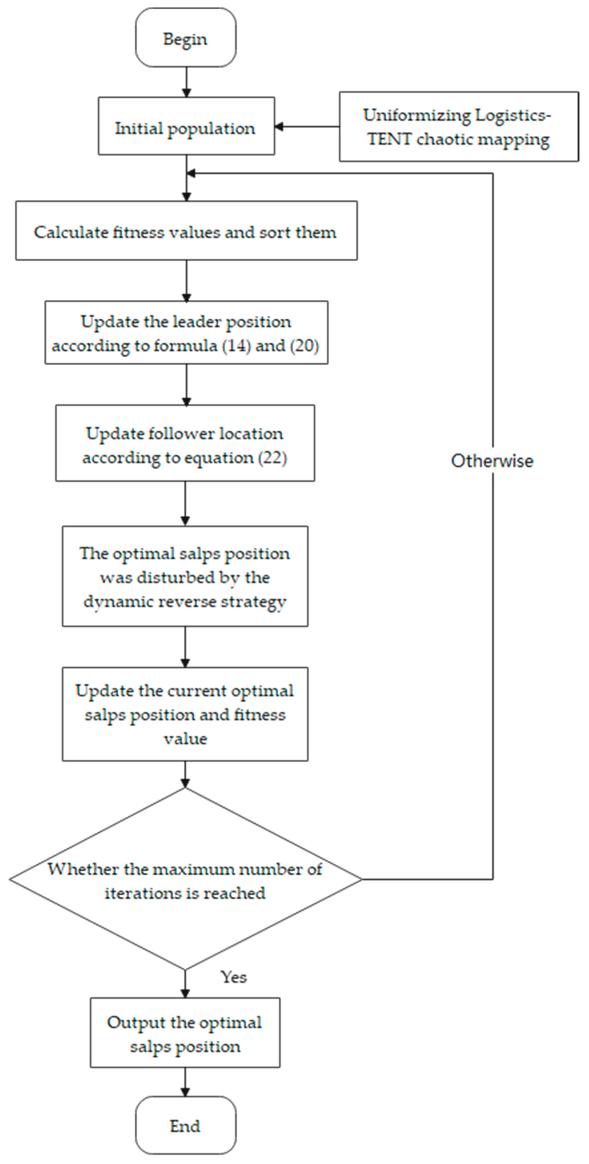
3.2. Improved Salp Swarm Algorithm

While the SSA is biologically-inspired and structurally simple to implement, it has some drawbacks and limitations, such as a lack of diversity, slow convergence, low solution accuracy, and a propensity to fall into local optima [28]. To address these issues, an ISSA is proposed, optimizing its global and local search capabilities. The improvements are made in the following four areas:

• Using logistic-tent chaotic mapping in place of random initialization of the salp swarm population, ensuring a more uniform distribution within the search space;
• Introducing adaptive parameters to balance the leader’s exploration and exploitation, enhancing the algorithm’s search scope in the early stages of iteration;
• Implementing an adaptive inertia weight factor for the followers’ positions to control the individual search scope and convergence speed while using an elite strategy to amplify the guiding effect of elite individuals;
• After updating the salps individual’s position, a dynamic reversal strategy is employed to perturb the salps with the updated optimal position, enhancing its search capability.

3.2.1. Logistic-Tent Chaotic Mapping

Chaos describes the characteristics of nonlinear systems. It exhibits high sensitivity to initial conditions, non-periodic behaviors, and randomness. This phenomenon is prevalent in both nature and human activities, playing a crucial role in many application domains.

During the initialization phase of the SSA, the population is generated randomly. Due to this randomness, the initial population quality might be unstable and lack diversity. Moreover, some individuals could be concentrated in less optimal areas of the search space, leading to slower convergence or individuals becoming trapped in local optima. By integrating chaotic mapping into the population initialization, its high randomness and extensive search range can enhance the population diversity and exploration space. Its adaptability and adjustability make it suitable for various problems and algorithmic needs, maintaining diversity and avoiding local optima, thus enhancing the algorithm’s global search capability.

Gao, Y. [29] integrated the classic one-dimensional logistic chaotic system with the tent chaotic system to create the logistic-tent composite chaotic system. This merged system combines the intricate chaotic dynamics of the logistic system with the tent system’s faster iteration speed, higher autocorrelation, and suitability for large sequences [30]. It possesses superior chaotic attributes and offers a more even distribution. Its expression is as follows:

$$x_{n+1}=\{\begin{array}{c}\left[r{x}_n\left(1-x_n\right)+\frac{\left(4-r\right)}{2}{x}_n\right]\mathrm{mod}1\begin{array}{cc},& \begin{array}{cc}if& x_n<0.5\end{array}\end{array}\\ \left[r{x}_n\left(1-x_n\right)+\frac{\left(4-r\right)}{2}{x}_n\right]\mathrm{mod}1\begin{array}{cc},& \begin{array}{cc}if& x_n\ge 0.5\end{array}\end{array}\end{array}$$

(18)

In this formula, $x$ represents the system variable and the chaotic value of the system, with $x\in [0,1]$; $r$ is the control parameter, and its range is $r\in (0,4)$. To make the chaos value distributed evenly, 0.3 is set in this study. To illustrate the distribution, the dimension $D=3$ is used as an example. After initializing the logistic-tent chaotic mapping and iterating it 1000 times, it is compared with random initialization. As shown in Figure 2 and Figure 3, the distribution of chaotic values and the frequency graphs of chaotic values in different dimensions are compared. It can be observed that the distribution of the logistic-tent chaotic mapping is relatively uniform, with fewer occurrences of extreme values.

3.2.2. Adaptive Parameters

From Equation (14), it is clear that the leader only updates its position relative to the food source. It is evident that the coefficient $c_1$ is the most crucial parameter in the SSA, as it strikes a balance between exploration and exploitation. However, the rapid decline during the algorithm’s iteration process can cause the algorithm to quickly enter the local search phase. To address this problem, an adaptive parameter $\sigma$ is introduced to enhance the search range in the early iterations of the algorithm. The expression for this parameter is as follows:

$${\sigma }^2=-4\ln \frac{x}{4}\begin{array}{cc}& x\in (0,2)\end{array}$$

(19)

When it is incorporated into Equation (15), the modified equation is obtained:

$$c_1=2e^{-{\left(\frac{\sigma L}{L_{\max }}\right)}^2}$$

(20)

To mitigate the decline of $c_1$, $x=0.3$ is set. Based on this setting, the value of $c_1$ is calculated. Comparing the values of $c_1$ before and after the modification, the resulting graph is as shown in Figure 4. By introducing the adaptive parameter, the rate of decline of $c_1$ is adjusted, based on the maximum number of iterations, ensuring a sufficiently broad search range in the initial stages of iteration.

From Figure 4., it is evident that, during the early iterations, the value $c_1$ is relatively high and decreases rapidly. This outcome facilitates an expansion of the search range of the SSA, enhancing its global search capabilities and accelerating its convergence speed. In the mid-phase of the iterations, the $c_1$ of the rate of decrease slows, bolstering the algorithm’s local search capabilities.

3.2.3. Adaptive Dynamic Inertia Weights and Elite Strategies

Incorporating an inertia weight can enhance the algorithm’s ability for local searches, expediting convergence and ensuring stability. At the same time, it strikes a balance between global exploration and local optimization. A larger inertia weight provides a stronger ability for global searching, while a smaller one excels in local exploitation [31]. Therefore, an adaptive inertia weight factor $\omega$ is introduced in the follower’s position to regulate the search scope and convergence rate of each individual. The calculation formula for the adaptive inertia weight factor $\omega$ is as follows:

$$\omega {(t)}_i=\{\begin{array}{ll}{\omega }_{\min }+\frac{\left({\omega }_{\max }-{\omega }_{\min }\right)\left(f{(t)}_i-f{(t)}_{\min }\right)}{f{(t)}_{avg}-f{(t)}_{\min }}& f{(t)}_i\le f{(t)}_{avg}\\ {\omega }_{\max }& f{(t)}_i>f{(t)}_{avg}\end{array}$$

(21)

In the formula, $\omega {(t)}_i$ represents the weight of individual $i$ in iteration $t$, and $f{(t)}_i$ denotes the fitness value of individual $i$ during iteration $t$. Meanwhile, $f{(t)}_{avg}$ and $f{(t)}_{\min }$ correspond to the average and minimum fitness values of all salps in iteration $t$, respectively. The ${\omega }_{\max }$ and ${\omega }_{\min }$ are the preset maximum and minimum inertia coefficients, respectively. According to the literature [32], they are typically set to ${\omega }_{\min }=0.4$, ${\omega }_{\max }=0.9$.

If the fitness of the current salp exceeds the average fitness, it suggests that it is close to the global optimum. In this case, a smaller inertia weight $\omega$ should be chosen to preserve its position. Conversely, if its fitness is less than the average, it may be far from the global optimum. At this point, a larger inertia weight should be selected to direct the salp toward a more favorable search area.

From Equation (17), it is evident that the follower updates its position based on the midpoint of the positions of salps $i$ and $i-1$. However, this update method overlooks the quality of the positions of the salp swarm individuals, resulting in a diminished guiding role of the elite individuals. To enhance the influence of elite individuals and maximize the information utility among individuals, thereby improving the algorithm’s convergence rate, an elite strategy is introduced into the follower position, updating the phase of the SSA. Coupled with the inertia weight, it perturbs inferior salp individuals, yielding the following formula:

$$X_j^i=\{\begin{array}{c}\frac{1}{2}(\omega X_j^i+X_j^{i-1})\begin{array}{cc}& f(X_j^i)>f(X_j^{i-1})\end{array}\\ \frac{1}{2}(X_j^i+X_j^{i-1})\begin{array}{cc}& f(X_j^i)=f(X_j^{i-1})\end{array}\\ \frac{1}{2}(X_j^i+\omega X_j^{i-1})\begin{array}{cc}& f(X_j^i)<f(X_j^{i-1})\end{array}\end{array}$$

(22)

where $f(X_j^i)$ represents the fitness value of individual $i$ in dimension $j$.

3.2.4. Dynamic Inversion Strategy

In the latter stages of the SSA, it is inevitable for the algorithm to fall into local optima due to the rapid convergence of individual solutions. To address this issue, an inversion learning strategy is introduced. After the salp individual’s search, a perturbation is applied to the salp individual. The fitness of both the current solution and its inverse solution is assessed. This approach enhances the algorithm’s optimization searching capability and increases the chances of escaping local optima. The inverse solution is given by:

$${(X_j^i(t))}^{*}=k(a_j^i(t)+b_j^i(t))-X_j^i(t)$$

(23)

In this equation, $a_j^i=\min (X_j^i(t))$ and $b_j^i=\max (X_j^i(t))$ represent the minimum and maximum values of dimension $j$ for individual $i$ in iteration $t$, respectively. $k$ is the inversion coefficient, which is a random number between 0 and 1.

3.2.5. Algorithm Flowchart

In this study, the optimization objectives include fluctuations under steady conditions and overshoot and time during transient conditions. Importance levels for optimization are determined by weight values. Therefore, the fitness function is formulated as shown in Equation (24).

$$f_{is}={\displaystyle \sum _{i=1}^m({\displaystyle {\int }_0^{\infty }{k}_1\left|e(i)\right|}+k_2\partial +k_3{t}_s)}\begin{array}{cc}& i=1,2,\cdots ,m\end{array}$$

(24)

where $e(t)$ represents the speed deviation; $\partial$ is the overshoot; $t_s$ denotes the settling time; and $k_1$, $k_2$ and $k_3$ are their respective weight values.

Based on the strategies mentioned, this study introduces improvements to the SSA, enhancing the algorithm’s exploration and exploitation capabilities. The resulting ISSA is depicted in the flowchart presented in Figure 5.

Step 1 (Initialization): Initialize the salp swarm population size $N$, maximum iteration count $L_{\max }$, upper bound of feasible solution $u{b}_j$, lower bound lower bound $l{b}_j$, problem dimension $D$, and the fitness function $f_{is}$.

Step 2 (Population initialization): Utilize the logistic-tent chaotic mapping to construct the initial population.

Step 3 (Fitness calculation): Calculate the fitness values for each salp individual.

Step 4 (Optimal sequence update): Sort the fitness values and determine the optimal fitness value, along with the best position of the salp.

Step 5 (Location Update): Update the positions of the leader and followers based on Equations (14), (20) and (22) respectively. Refresh the optimal fitness value and the best position accordingly.

Step 6 (Location Update): Employ the dynamic reverse strategy to perturb the optimal salp position, and subsequently update the best position and optimal fitness value.

Step 7 (Iteration termination condition judgment): If the iteration reaches the maximum number of iterations, output the global optimal fitness function value and the global optimal position. Otherwise, return to Step 3 and continue the loop.

To validate the performance and optimization results of the improved salp swarm algorithm, eight benchmark functions with distinct optimization characteristics are selected [33,34,35]. These functions were tested under $D=30$ dimensions with the population size of 50 to evaluate the refined algorithm, as shown in

Table 2. Benchmark Functions.

Function Name	Function	Section	Starter
Sphere F	$F_1(x)={\displaystyle \sum _{i=1}^D{x}_i^2}$	[−100, 100]	0
Schwefel’s P2.22	$F_2(x)={\displaystyle \sum _{i=1}^D\left|x_i\right|}+{\displaystyle \prod _{i=1}^D\left|x_i\right|}$	[−10, 10]	0
Schwefel’s P1.2	$F_3(x)={{\displaystyle \sum _{i=1}^D\left({\displaystyle \sum _{j=1}^i{x}_j}\right)}}^2$	[−100, 100]	0
Schwefel’s P2.21	$F_4(x)={\max }_i\{\left|x_i\right|,1\le i\le D\}$	[−100, 100]	0
Generalized Schwefel’s P2.26	$F_5(x)={\displaystyle \sum _{i=1}^D-x_i\sin \sqrt{\left|x_i\right|}}$	[−500, 500]	0
Generalized Rastrigin’s F	$\begin{array}{l}{F}_6(x)=-20e^{(-0.2\sqrt{\frac{1}{n}{\displaystyle {\sum }_{i=1}^D{x}_i{}^2}})}\\ -e^{(\frac{1}{n}{\displaystyle {\sum }_{i=1}^D\cos (2\pi x_i)})}\end{array}$	[−5.12, 5.12]	0
Ackley’s F	$\begin{array}{l}{F}_7(x)=-20e^{(-0.2\sqrt{\frac{1}{n}{\displaystyle {\sum }_{i=1}^D{x}_i{}^2}})}\\ -e^{(\frac{1}{n}{\displaystyle {\sum }_{i=1}^D\cos (2\pi x_i)})}\end{array}$	[−32, 32]	0
Generalized Griewank’s F	$\begin{array}{l}{F}_8(x)=\frac{1}{4000}{\displaystyle \sum _{i=1}^D{x}_i{}^2}\\ -{\displaystyle \prod _{i=1}^D\cos (\frac{x_i}{\sqrt{i}})+1}\end{array}$	[−600, 600]	0

. Functions F1 to F4 are unimodal functions, effectively testing the algorithm’s global search capability; while functions F5 to F8 are multimodal functions, providing a solid test of the algorithm’s convergence speed and accuracy [36].

In the comparison, the LTSSA represents the SSA integrated with logistic-tent chaotic mapping, termed the logistic-tent chaotic mapping salp swarm algorithm. ASSA stands for the adaptive parameter salp swarm algorithm, which introduces adaptive parameters. WSSA, the inertia weight salp swarm algorithm, incorporates an adaptive dynamic inertia weight and elite strategy. DSSA, or the dynamic inverse strategy salp swarm algorithm, introduces a dynamic inverse strategy. Figure 6 displays the comparative convergence curve results, where the x-axis represents the number of iterations, and the y-axis denotes the fitness value. As shown in the figure, singular optimizations generally enhance the performance of the SSA to some extent. Moreover, at the beginning of the iteration, the ISSA tends to converge to the optimal solution faster than the LTSSA in most cases. However, when compared to the LTSSA, ASSA, WSSA, and DSSA, which each incorporate individual optimization techniques, the ISSA algorithm proposed in this study demonstrates faster convergence speed and greater precision.

Table 3. The Optimization Result of the Benchmark Function.

	Algorithm	SSA	LTSSA	ASSA	WSSA	DSSA	ISSA
Function
F1		3.7 × 10−2	7.28 × 10−9	7.29 × 10−9	1.04 × 10−7	1.48 × 10−8	7.98 × 10−11
F2		1.37	2 × 10−2	1.9 × 10−2	4.81 × 10−5	9.5 × 10−2	3.18 × 10−6
F3		3.4 × 101	7.46 × 10−1	7.8 × 101	1.27 × 10−8	1 × 102	1.74 × 10−10
F4		1.07 × 101	1.86 × 10−2	2.75 × 101	3.7 × 10−5	2.98 × 101	2.46 × 10−6
F5		−8.28 × 103	−6.06 × 103	−7.37 × 103	−7.01 × 103	−8.44 × 103	−1.25 × 104
F6		5.07 × 101	4.97 × 10−9	6.37 × 101	6.39 × 10−9	4.28 × 101	4.03 × 10−11
F7		2.12	2.34 × 10−5	2.41	2.31 × 10−5	1.65	1.84 × 10−6
F8		3.47 × 10−8	1.23 × 10−2	4.65 × 10−2	4.97 × 10−8	1.15	2.86 × 10−10

presents the extreme values of the best fitness for various algorithms after 1000 iterations.

4. Diesel Engine Speed Control Simulation Analysis

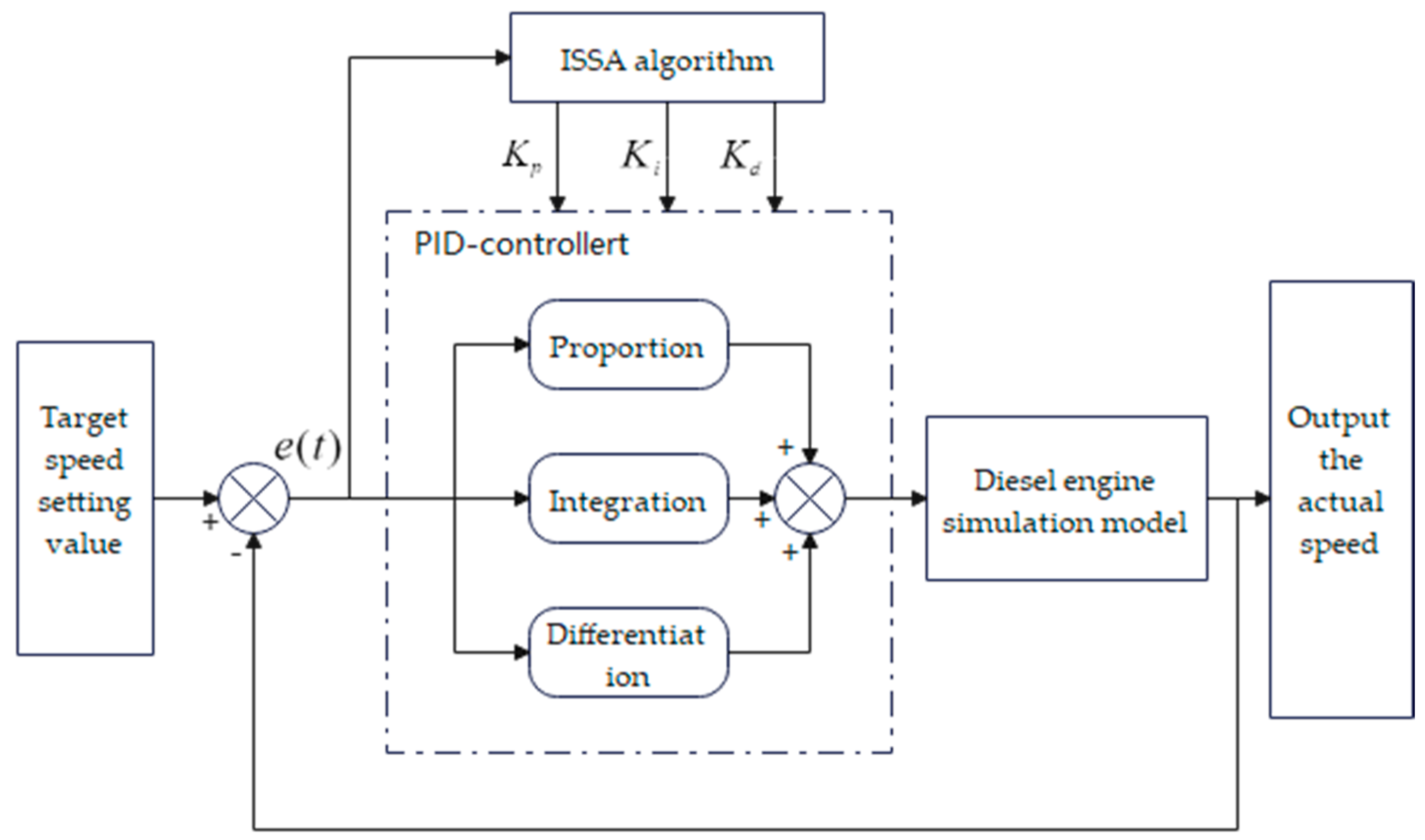
4.1. Principle of PID Control System Optimization Based on ISSA Algorithm

During the actual operation of the engine, the ECU determines the target speed based on the current operating conditions. The current engine speed is then acquired through a speed sensor, serving as the feedback signal for the PID controller. The controller next calculates the discrepancy between the target and actual speeds. The proportional control generates an output signal based on the speed error, the integral control does so based on the accumulated value of the speed error, and the derivative control responds to the rate of change of the speed error. Subsequently, the outputs from the proportional, integral, and derivative components are weighted and totaled to form the final output signal of the PID controller. This output signal adjusts control parameters, such as fuel supply and valve opening, to achieve the desired speed control. In this study, the PID controller parameters of the system are optimized based on speed deviations using the ISSA. This optimization aims to reduce speed fluctuations in steady-state conditions and overspeed and stabilization time during dynamic conditions, thereby enhancing engine performance. The schematic of the diesel engine speed control system, based on the improved ISSA designed in this study, is shown in Figure 7.

4.2. Model Simulation Accuracy Verification

To ensure the accuracy of the diesel engine simulation model, the model simulation data were compared with experimental data. The fuel injection quantities were verified at 1200 r/min, 1600 r/min, and 2200 r/min under different torques, as shown in Figure 8. The maximum error was 8.9%, and the average error was 4.2%. The results indicate that the established diesel engine simulation model can be used for the verification of control algorithms.

4.3. Simulation Test of Speed Tracking Performance

In the MATLAB/Simulink environment, the algorithm code was integrated with the constructed diesel engine model to implement mirror simulation. To validate the feasibility and effectiveness of the ISSA-PID control algorithm, drawing upon the comparison methods from references [20,21], simulation tests were conducted at common operating points of the diesel engine. The ISSA was compared with the particle swarm optimization (PSO) algorithm and incremental PID tuning. The simulation process included set speed step-change simulation tests and load step-change simulation tests.

4.3.1. Speed Step-Change Simulation Test

When the engine load is set to 50%, the speed is maintained at 1000 r/min for a period of time before increasing to 1400 r/min and then dropping back to 1000 r/min. Subsequently, under a 30% load, after the speed stabilizes at 2000 r/min, it is increased to 2400 r/min and then decreases back to 2000 r/min. Tests were conducted for 70 s under each of the four control algorithms, with a calculation step size of 0.001 s. Data from 50 s of testing under each condition were selected, and the comparison results are shown in Figure 9.

From the figure, it is evident that the ISSA showcases superior control performance during sudden engine speed changes compared to other algorithms. Calculations reveal that, when speed suddenly increases, under a 50% load, the overshoot is reduced by 13.4%, 62.6%, and 14.9% compared to SSA, PSO, and engineering tuning methods, respectively. The settling time decreased by 0.24 s and 3.11 s when compared to the SSA and the engineering tuning method, respectively, but increased by 1.06 s compared to the PSO method. Under a 30% load, the overshoot decreased by 22.2%, 61.1%, and 32.4%, respectively. The settling time, in comparison to the SSA and engineering tuning, decreased by 0.69 s and 0.99 s, respectively, while it remained almost consistent with the PSO method. Although there are instances of shorter settling times, the significantly reduced overshoot compensates for any impact due to settling time.

4.3.2. Load Surge Simulation Test

Under a set engine speed of 1200 r/min, after allowing the speed to stabilize for a while, the load is increased from 60% to 90% and then returns to 60%. Subsequently, at 2400 r/min, the load is raised from 20% to 50%, and once the speed stabilizes, it is reduced back to 20%. Four control algorithms were tested for a duration of 70 s each, with a calculation timestep of 0.001 s. Data from 50 s of the tests for each condition were selected for comparison, as shown in Figure 10.

From the figure, it is evident that the ISSA outperforms other methods in terms of control performance when the engine load undergoes sudden changes. Calculations reveal that, during a sudden increase in speed, at 1200 r/min, the overshoot is reduced by 15.3%, 30.8%, and 37.1% compared to the SSA, PSO, and the engineering tuning method, respectively. The settling time decreases by 3.79 s and 2.11 s when compared to the SSA and the engineering tuning method, respectively, but it increases by 1.34 s when compared to the PSO method. At 2400 r/min, the overshoot is reduced by 18.9% and 8% when compared to the SSA and the engineering tuning method, respectively, and increases by 1.14% in comparison to the PSO method. The settling time decreases by 3.61 s and 1.12 s compared to PSO and the engineering tuning method, respectively, but rises by 0.41 s compared to the SSA. Although there are situations with lower overshoot and settling times, the balanced overshoot and settling times counteract each other’s effects.

5. Conclusions

To better regulate the diesel engine’s speed, a method based on the improved salp swarm algorithm for PID optimization was proposed. This method was then applied to tune the parameters of a diesel engine model’s PID controller. The following conclusions were drawn after validating with experimental data:

• To address the issues of reduced population diversity and the tendency to become trapped in local optima in the salp swarm algorithm, the algorithm was tested, both before and after improvements, using various benchmark functions. The test results on these benchmark functions showed that the improved salp swarm algorithm significantly enhances both global and local search capabilities. It effectively prevents the algorithm from becoming stuck in local optima, validating the feasibility and effectiveness of the improved approach;
• Utilizing the improved salp swarm algorithm for PID control parameter optimization led to reductions in speed overshoot and stabilization time. During sudden speed changes at 50% and 30% load, the ISSA, compared to the SSA, PSO, and engineering tuning methods, averaged reductions of 30.3% and 38.6% in overshoot and of 0.76 s and 0.84 s in stabilization time, respectively. When the load underwent abrupt changes, the ISSA, at speeds of 1200 r/min and 2400 r/min, reduced the overshoot by an average of 27.7% and 8.6%, respectively, and the stabilization time by an average of 1.52 s and 4.32 s. ISSA offers a more balanced control performance and, compared to the other three methods, excels in stable speed control and rapid response. Moreover, the system achieves faster stabilization times, proving its valuable significance in engineering applications.

References

1. Astrom, K.; Hagglund, T. The Future of PID Control. IFAC Proc. Vol. 2000, 33, 19–30. [Google Scholar] [CrossRef]
2. Parada, M.; Sbarbaro, D.; Borges, R.; Peres, P. Robust PI and PID Design for First- and Second-Order Processes with Zeros, Time-Delay and Structured Uncertainties. Int. J. Syst. Sci. 2017, 48, 95–106. [Google Scholar] [CrossRef]
3. Garpinger, O.; Hgglund, T.; Strm, K.J. Performance and robustness trade-offs in PID control. J. Process Control 2014, 24, 568–577. [Google Scholar] [CrossRef]
4. Li, Y.; Xu, F.J.; Wang, B. Experimental Study on Loaded Suddenly and Unloaded Suddenly of 16 V Generator Diesel. Mod. Veh. Power 2015, 157, 27–29, 34. [Google Scholar]
5. Astrom, K.J.; Hagglund, T. Automatic tuning of simple regulators with specifications on phase and amplitude margins. Automatica 1984, 20, 645–651. [Google Scholar] [CrossRef]
6. Kiam, H.A.; Chong, G.; Li, Y. PID control system analysis, design, and technology. IEEE Trans. Control Syst. Technol. 2005, 13, 559–576. [Google Scholar] [CrossRef]
7. Chen, Y.Q.; Moore, K.L. Relay feedback tuning of robust PID controllers with iso-damping property. IEEE Trans. Syst. Man Cybern. Part B 2005, 35, 23–31. [Google Scholar] [CrossRef]
8. Hernández-Alvarado, R.; García-Valdovinos, L.; Salgado-Jiménez, T.; Gómez-Espinosa, A.; Fonseca-Navarro, F. Neural Network-Based Self-Tuning PID Control for Underwater Vehicles. Sensors 2016, 16, 1429. [Google Scholar] [CrossRef] [PubMed]
9. Meena, D.C.; Devanshu, A. Genetic algorithm tuned PID controller for process control. In Proceedings of the 2017 International Conference on Inventive Systems and Control (ICISC), Coimbatore, India, 19–20 January 2017; pp. 1–6. [Google Scholar] [CrossRef]
10. Abushawish, E.A.; Hamadeh, M.; Nassif, A. PID Controller Gains Tuning Using Metaheuristic Optimization Methods: A survey. Int. J. Comput. 2020, 14, 87–95. [Google Scholar] [CrossRef]
11. Sun, W.F.; Liu, H.Y.; Wang, R.T.; Fu, T.P.; Lu, J.Q.; Wang, F.L. Design and Experiment of PID Control Variable Application System Based on Neural Network Tuning. Trans. Chin. Soc. Agric. Mach. 2020, 51, 55–64, 94. [Google Scholar]
12. Feng, J.X.; Wang, Q.; Wang, Y.L.; Xu, B. Fuzzy PID control of ultrasonic motor based on improved quantum genetic algorithm. J. Jilin Univ. Eng. Technol. Ed. 2021, 51, 1990–1996. [Google Scholar]
13. Zhai, M.D.; Zhang, B.; Li, X.L.; Long, Z.Q. Design and Implementation of Magnetic Suspension Vibration Isolation Platform with Quasi-Zero Stiffness Based on Fuzzy PID Control. J. Southwest Jiaotong Univ. 2023, 58, 886–895. [Google Scholar]
14. Seyyed, M.H.; Ramin, F. Intelligent VIV control of 2DOF sprung cylinder in laminar shear-thinning and shear-thickening cross-flow based on self-tuning fuzzy PID algorithm. Mar. Struct. 2023, 89, 103377. [Google Scholar]
15. Zhang, J.H.; Li, Y.M.; Qi, W.C.; Liu, C.L.; Yang, F.Z.; Li, Z.P. Synchronous Control System of Tractor Attitude in Hills and Mountains Based on Neural Network PID. Trans. Chin. Soc. Agric. Mach. 2020, 51, 356–366. [Google Scholar]
16. Jiang, X.H.; Cheng, T.H. Design of a BP neural network PID controller for an air suspension system by considering the stiffness of rubber bellows. Alex. Eng. J. 2023, 74, 65–78. [Google Scholar] [CrossRef]
17. Shi, J.Z.; Liu, Y. Simple Expert PID Speed Control of Ultrasonic Motors. Proc. CSEE 2013, 33, 120–126. [Google Scholar]
18. Miao, R.L.; Dong, Z.P.; Wan, L.; Zeng, J.F. Heading Control System Design for a Micro-USV Based on an Adaptive Expert S-PID Algorithm. Pol. Marit. Res. 2018, 25, 13–16. [Google Scholar] [CrossRef]
19. Matsumoto, H.; Morita, S.; Takiyama, T. Application of Fuzzy Control to Internal Combustion Engines. JSME Int. J. Ser. B-Fluids Therm. Eng. 1994, 37, 159–164. [Google Scholar] [CrossRef]
20. Shao, C.; Song, K.; Cheng, T.; Xie, H. Active Disturbance Rejection Control of Diesel Engine Speed Based on Parameter Self-Learning. Trans. CSICE 2022, 40, 144–152. [Google Scholar]
21. Song, E.Z.; Song, T.K.; Ma, C.; Yao, C.; Liu, Z.L. Research on Diesel Engine Speed Control Based on Model Reference Adaptive. Chin. Intern. Combust. Engine Eng. 2022, 43, 57–64. [Google Scholar]
22. Liang, J.J.; Qin, A.K.; Suganthan, P.N.; Baskar, S. Comprehensive learning particle swarm optimizer for global optimization of multimodal functions. IEEE Trans. Evol. Comput. 2006, 10, 281–295. [Google Scholar] [CrossRef]
23. Zamani, M.; Karimi-Ghartemani, M.; Sadati, N.; Mostafa, P. Design of a fractional order PID controller for an AVR using particle swarm optimization. Control. Eng. Pract. 2009, 17, 1380–1387. [Google Scholar] [CrossRef]
24. Xiang, H.C.; Ma, Z.T.; Yang, Z.T.; Yang, M.Y.; Deng, K.Y.; Huang, M.; Liu, Y. Performance Response Characteristic of Turbocharged Diesel Engine Under Fluctuating HighBack Pressure Environment. Trans. CSICE 2023, 41, 404–411. [Google Scholar]
25. Lei, L.; Yu, Y.H.; Shen, L.Z.; Wan, M.D.; Huang, F.L.; Wang, Z.J. Investigation on Transient Emissions of Diesel Engine at Different Altitudes. Trans. CSICE 2023, 41, 420–426. [Google Scholar]
26. Shah, R.K.; Sekulic, D.P. Fundamentals of Heat Exchanger Design; John Wiley and Sons: Hoboken, NJ, USA, 2003. [Google Scholar]
27. Seyedali, M.; Amir, H.G.; Seyedeh, Z.M.; Shahrzad, S.; Hossam, F.; Seyed, M.M. Salp Swarm Algorithm: A bio-inspired optimizer for engineering design problems. Adv. Eng. Softw. 2017, 114, 163–191. [Google Scholar]
28. Cheng, Y.X.; Zhang, T.; Liu, Y.G.; Chen, J. Lightweight Design Method of Girder Hoist Based on Improved Salp Swarm Algorithm. J. Northeast. Univ. Nat. Sci. 2023, 44, 223–232. [Google Scholar]
29. Gao, Y. Pseudorandom Sequence IP Design Based on Logistic Chaos Algorithm; Heilongjiang University: Harbin, China, 2021. [Google Scholar]
30. Qin, Q.X.; Liang, Z.Y.; Xu, Y. Image Encryption Algorithm Based on Logistic-Tent Chaotic Mapping and Bit Plane. J. Dalian Minzu Univ. 2022, 24, 245–252. [Google Scholar]
31. Shi, Y.; Eberhart, R. A modified particle swarm optimizer. In Proceedings of the 1998 IEEE International Conference on Evolutionary Computation Proceedings, IEEE World Congress on Computational Intelligence (Cat. No.98TH8360), Anchorage, AK, USA, 4–9 May 1998; pp. 69–73. [Google Scholar]
32. Lian, X.Q.; Liu, Y.; Chen, Y.M. Research on Multi-Peak Spectral Line Separation Method Based on Adaptive Particle Swarm Optimization. Spectrosc. Spectr. Anal. 2021, 41, 1452–1457. [Google Scholar]
33. Feng, Z.X.; Li, J.L.; Ge, X.; Zhou, Y.J. Integrating multi strategy improved whale optimization algorithm and its application. Comput. Integr. Manuf. Syst. 2023, 1–23. [Google Scholar]
34. Zeng, N.Y.; Song, D.D.; Li, H.; Yan, C.; You, Y.C. Improved Whale Optimization Algorithm and Turbine Disk Structure Optimization. J. Mech. Eng. 2021, 51, 254–265. [Google Scholar]
35. Li, Y.L.; Wang, S.Q.; Chen, Q.R.; Wang, X.G. Comparative Study of Several New Swarm Intelligence Optimization Algorithms. Comput. Eng. Appl. 2020, 56, 1–12. [Google Scholar]
36. Li, J.L.; Wang, G.Y.; Wang, Y.H.; Deng, D.R.; Zhao, Y.; He, S.C. Research on Diesel Engine Common Rail Pressure Control Based on Gaussian-Cauchy Mutation Seagull Optimization Algorithm. Chin. Intern. Combust. Engine Eng. 2022, 43, 16–25. [Google Scholar]
Figure 1. Diesel engine model system framework.
Processes 11 03092 g001
Figure 2. Random initialization chaotic value distribution diagram and chaotic value frequency diagram in different dimensions. (a) Chaotic value distribution diagram. (b) Chaotic value frequency graph.
Processes 11 03092 g002
Figure 3. Logistic-tent chaotic map initializes the distribution of chaotic values and the frequency of chaotic values in different dimensions. (a) Chaotic value distribution diagram. (b) Chaotic value frequency graph.
Processes 11 03092 g003
Figure 4. c 1 comparison before and after improvement.
Processes 11 03092 g004
Figure 5. Improved salp swarm algorithm workflow.
Processes 11 03092 g005
Figure 6. Convergence plot from the benchmark experiments. (a) F1. (b) F2. (c) F3. (d) F4. (e) F5. (f) F6. (g) F7. (h) F8.
Processes 11 03092 g006
Figure 7. Schematic of the PID control system based on the ISSA.
Processes 11 03092 g007
Figure 8. Comparison of cycle fuel injection between simulation and experimental data. (a) 1000 r/min; (b) 1600 r/min; (c) 2200 r/min.
Processes 11 03092 g008
Figure 9. Speed transition comparison under different loads. (a) Comparison of speed mutation under 50% load. (b) Comparison of speed mutation under 30% load.
Processes 11 03092 g009
Figure 10. Speed comparison during sudden load changes at different engine speeds. (a) Comparison of speed when load changes at 1200 r/min. (b) Comparison of speed when load changes at 2400 r/min.
Processes 11 03092 g010