Simulation Analysis of the Characteristics of Layered Cores during Pulse Decay Tests

Abstract

The permeability of low-permeability cores is generally measured using a pulse decay method. The core of low-permeability rocks, such as shale, often has a layered structure. The applicability of pulse decay testing for layered cores is not clear. In this study, the performance of the pulse decay method on layered cores was comprehensively investigated. Numerical simulations were conducted to investigate the influence of the interlayer permeability ratio, storativity ratio, layer thickness, interlayer location, and number of layers on the pulse decay pressure and pressure derivative curves, as well as the permeability obtained from pulse decay testing. The results revealed that the pressure curves of layered cores exhibit distinct differences from those of homogeneous cores if the upstream permeability is larger than the downstream one. The pressure derivative curve shows more inclined or horizontal straight-line segments than in the homogeneous case. The shapes of the pressure and pressure derivative curves are affected by the upstream and downstream positions of the core, but the tested permeability is not affected. The tested permeability differs from the equivalent model permeability, with an error of up to 22%. If the number of layers is not less than 10, the permeability obtained from the pulse decay test is consistent with that of the equivalent model. These differences are influenced by the interlayer permeability ratio, storativity ratio, layer thickness, interlayer location, and number of layers. To improve the accuracy of permeability analysis in pulse decay testing for layered cores, curve fitting using the characteristics of the pressure derivative curve can be employed.

1. Introduction

The testing of rock permeability is often encountered in hydraulic engineering, petroleum engineering, coal bed methane (CBM) engineering, underground engineering and so on [1,2]. The methods for measuring rock permeability include the steady-state method and transient method [3,4]. For low-permeability cores, the steady state method is time-consuming, so the transient method is generally adopted. The pulse decay method is the most common transient method for permeability testing [5,6]. The method uses two pressure vessels, one upstream and one downstream. The upstream and downstream pressure and core pressure are balanced at the beginning. Then, a pressure pulse is applied at the upstream, and the core permeability is obtained by analyzing the change in upstream and downstream pressures over time (Figure 1). As Brace et al. [7] tested granite permeability using the pulse decay method in 1968, this method has been widely used and improved, becoming a standard method for testing low-permeability cores. An analytical solution for the pulse decay testing of homogeneous core was presented by Hsieh et al. [8]. This analytical solution was simplified, and a practical analytical method was proposed by Jones [9]. The permeability is obtained by analyzing the slope of the semi-logarithmic straight line of the pressure difference between the upstream and downstream in the later stage. Recently, Wang et al. [10] proposed an analysis method using the intercept of this straight line. The early and late asymptotic solutions of pulse decay testing are the main tools for the permeability analysis, and there have been continuous improvements [11,12,13]. These are all based on linear governing equations. When a large differential pressure is applied, or the slippage effect is significant, the permeability is a function of pressure, and the governing equation is nonlinear. The globally convergent least squares method was used by Zhao et al. [14] to analyze pulse decay tests under large pressure differences. Wang et al. [15] obtained an analytical solution for the late time stage considering pressure-dependent permeability through perturbation methods. An analytical model proposed by Tian et al. [16] takes the inertial effect and gas slippage effect caused by large differential pressures into account.

However, these methods did not consider the adsorption of gases by the cores. Over the past two decades, the exploitation of shale gas and coalbed methane has increased the significance of testing adsorbed gas permeability [17]. Cui [18] was the first to modify the analytical method for pulse decay testing to consider gas adsorption. Han et al. [19] further considered the influence of the adsorbed phase volume, and analysis methods for equilibrium adsorption and non-equilibrium adsorption were proposed.

Figure 1. Schematic of equipment for pulse decay testing [19].

Figure 1. Schematic of equipment for pulse decay testing [19].

The tested cores are not always homogeneous, often exhibiting structures. Considering the wide pore size distribution and mineralogical heterogeneity within shale matrix, Chen and Liu [20] established an analytical model for the later behavior of pulse decay testing using a dual-continuum medium. However, it is required that the volumes of upstream and downstream reservoirs are equal. Later, the model was improved to general cases with unequal volumes of upstream and downstream reservoirs [21]. Jia et al. [22] simulated pulse decay tests on rock cores containing fractures and Vugs and found that the pulse decay curves exhibited a dual-porosity behavior. The experiments they conducted showed that core heterogeneity has a significant impact on the early response of pulse decay testing, and the porosities obtained from the forward and backward flow tests are different, but little effect on the permeability was indicated from the later-stage data [23]. Arnoaimi et al. [24,25] carried out pulse decay experiments and numerical simulations on Eagle Ford and Haynesville shale samples containing microcracks. A dual-porosity model was used in the simulation to characterize micropores and microcracks. Through historical match results, the flow laws and pore volumes of fluids in different types of pores, as well as the different flow regime of He and CO₂ in shale, were analyzed. Croin et al. [26,27,28] conducted pulse decay tests on Barnett shale cores, which were composed of alternating layers of silty claystone and claystone. The anisotropic permeability and cm-scale dual-permeability phenomena were observed. These are attributed to the heterogeneity caused by shale strategic layering. Kamath et al. [29] were the first to study the pulse decay testing of fractured cores and found that the pressures of upstream and downstream continue to decrease together after reaching equilibrium until a final balance is archived. Ning et al. [30] proposed an analytical solution for pulse decay tests in cores with a penetrating fracture. A similar phenomenon has also been observed by Alnoaimi et al. [24] in shale cores and in layered cores by Cronin et al. [26]. Han et al. [31] analyzed this phenomenon using a dual-medium model, and the pressure derivative method was proposed for the analysis of testing results. The core structure can be identified by the pressure derivative method using early data, avoiding stopping the test when the upstream and downstream pressures reached equilibrium. The model parameter fitting is more convenient with the facilitation of the pressure derivative. Sedimentary rocks often exhibit a layered structure. For layered cores, the permeability anisotropy is significant. The dual medium model is only suitable for analyzing the permeability parallel to the bedding. Kamath et al. [29] was the first to conduct simulations and experiments investigation on pulse decay testing of layered heterogeneous cores. They simulated interference testing and found significant differences in the pressure curves between forward and reverse directions. However, they only conducted simulation analysis of one scenario and testing of one sample. Although anisotropic permeability was obtained in many studies using pulse decay testing and attributed it to the layered structure of cores [32,33], the applicability of pulse decay testing for a layered core has not been thoroughly analyzed at present. Therefore, there is still a lack of in-depth investigation on pulse decay testing for layered cores and analysis methods for the permeability perpendicular to the bedding.

Considering the progress in the pulse decay method (

Table 1. Overview of progress in the pulse decay method.

Author	Year	Contribution
Brace et al. [7]	1968	The pulse decay testing method was firstly used to measure core permeability.
Hsieh et al. [8]	1981	An accurate analytical solution for pulse decay testing was proposed.
Kamath et al. [29]	1992	The earliest research on pulse decay testing of fractured and heterogeneous cores.
Ning et al. [30]	1993	An analytical method for pulse decay testing of core with penetrating fractures is presented.
Jones [9]	1997	Proposed the most popular semi-logarithmic analysis method for pulse decay testing.
Cui et al. [18]	2009	Proposed an analysis method considering gas adsorption for pulse decay testing.
Bhandari et al. [27]	2015	The horizontal and vertical permeability of shale were measured by pulse decay method.
Cronin et al.	2016	Pulse decay tests were conducted on alternating layers of silty claystone and claystone cores, and anisotropic permeability and dual-permeability phenomena were observed.
Han et al. [31]	2018	The pressure derivative analysis method was proposed for the analysis of pulse decay testing.
Alnoaimi et al. [24]	2019	Comparative study of He and CO2 flows through shale cores using pulse decay tests.
Tian et al. [16]	2023	Takes the inertial effect and gas slippage effect caused by large differential pressures into account.
Wang et al. [15]	2023	Obtained an analytical solution for the late time stage considering pressure-dependent permeability.

), this study conducted numerical simulation to analyze the pressure and pressure derivative curves of pulse decay testing of two-layer, three-layer, and multi-layer cores. The characteristics of pressure and pressure derivatives of layered cores were identified. The pulse decay testing analysis method proposed by Jones [9] was applied to analyze the simulated data and was compared with the equivalent permeability model of layered cores. Lastly, a suggested analysis method for the pulse decay permeability of layered rock cores was provided.

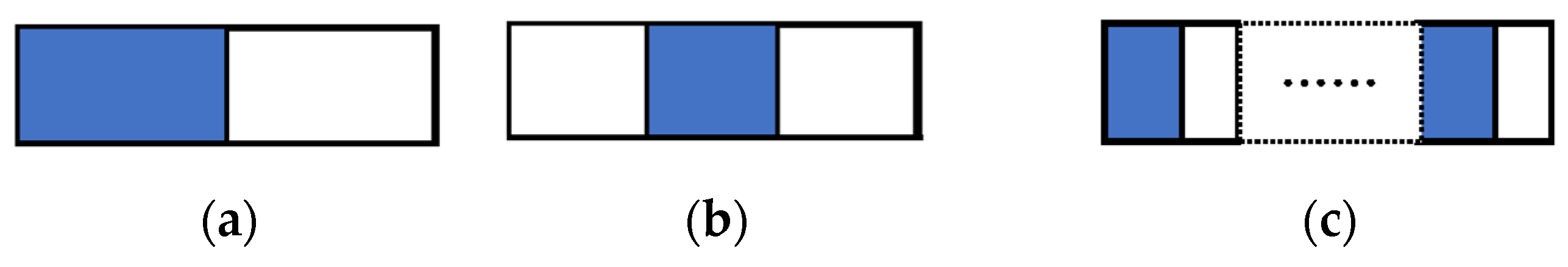
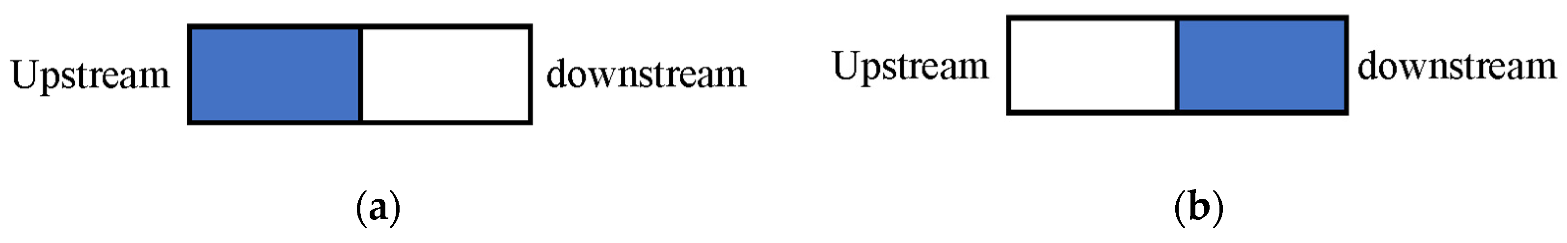
2. Definitions and Simulation Method

Layered rock cores are composed of multiple layers with different permeabilities, with alternating layers of two different permeabilities being quite common. For ease of study, it is assumed that the core consists of two layers with different permeabilities. One of the permeabilities is chosen as the reference permeability, whereas the ratio of other layer permeability to the reference permeability is varied. Due to differences in layer thickness, core size, and coring location, the composition of the core varies. The combination of two permeability layers is considered as follows: (1) a core composed of two layers; (2) a three-layer structure; and (3) a multi-layer core composed of alternating two types of permeability with equal thickness (Figure 2).

The permeability ratio is defined as follows:

$$p_{\mathrm{r}}=\frac{k_{\mathrm{v}}}{k_0}$$

(1)

where k₀ is the reference permeability, and k_v is the variable permeability, which are represented in white and blue, respectively, in Figure 2.

The core is tested using the setup shown in Figure 1. During the test, fluid flows from the upstream reservoir through the core to the downstream reservoir. For a single test using He with a small pressure pulse, it is appropriate to assume that the flow follows Darcy’s law. As the flow direction is perpendicular to the bedding, Darcy’s law is followed at each layer, but the parameters are different at each layer. The connection between layers has no effect on the flow. The governing equation for pulse decay testing is as follows [3,5,9]:

$$\varphi \mu c_{\mathrm{t}}\frac{\partial p}{\partial t}=\frac{\partial }{\partial x}\left(k\frac{\partial p}{\partial x}\right)$$

(2)

where p is the pressure in the core, t is the time, k is the core permeability, ϕ is the porosity, μ is the viscosity, c_t is the total compressibility, and x is the coordinate along the core length taking the upstream as the origin. Equation (2) is the governing equation for pulse decay testing. The initial conditions are as follows:

$$p\left(x,0\right)=p_{\mathrm{d}}\left(0\right),\begin{array}{cc}& 0<x\le L\end{array}$$

(3)

$$p\left(0,0\right)=p_{\mathrm{u}}\left(0\right)$$

(4)

where L is the core length, and p_u and p_d are the pressures of upstream and downstream vessels, respectively. The boundary conditions of the upstream and downstream are as follows:

$$\frac{\mathrm{d}{p}_{\mathrm{u}}}{\mathrm{d}t}={\frac{k}{\left(c_{\mathrm{L}}+c_{\mathrm{u}}\right)\mu {\left(\varphi L\right)}_{\mathrm{t}}}\frac{V_{\mathrm{p}}}{V_{\mathrm{u}}}\frac{\partial p}{\partial x}|}_{x=0},\begin{array}{cc}& t>0\end{array}$$

(5)

$$\frac{\mathrm{d}{p}_{\mathrm{d}}}{\mathrm{d}t}=-{\frac{k}{\left(c_{\mathrm{L}}+c_{\mathrm{d}}\right)\mu {\left(\varphi L\right)}_{\mathrm{t}}}\frac{V_{\mathrm{p}}}{V_{\mathrm{d}}}\frac{\partial p}{\partial x}|}_{x=L},\begin{array}{cc}& t>0\end{array}$$

(6)

where c_L is the compressibility of the testing fluid, c_u and c_d are the compressibility of the upstream and downstream vessels, V_p is the pore volume of the core, and V_u and V_d are the volumes of the upstream and downstream vessels, respectively. Dimensionless variables are defined as follows:

$$\begin{gathered} x_{\mathrm{D}}=\frac{x}{L}, A_{\mathrm{u}}=\frac{V_p{\left(\varphi c_{\mathrm{t}}{l}_i\right)}_{\mathrm{t}}}{V_{\mathrm{u}}\left(c_{\mathrm{L}}+c_{\mathrm{u}}\right){\left(\varphi l_i\right)}_{\mathrm{t}}}, A_{\mathrm{d}}=\frac{V_p{\left(\varphi c_{\mathrm{t}}{l}_i\right)}_{\mathrm{t}}}{V_{\mathrm{d}}\left(c_{\mathrm{L}}+c_{\mathrm{u}}\right){\left(\varphi l_i\right)}_{\mathrm{t}}}, \\ \omega =\frac{\varphi c_{\mathrm{t}}L}{{\left(\varphi c_{\mathrm{t}}{l}_i\right)}_{\mathrm{t}}},p_{\mathrm{D}}=\frac{p}{p_{\mathrm{d}}\left(0\right)}, t_{\mathrm{D}}=\frac{k_{0}t}{\mu {\left(\varphi c_{\mathrm{t}}{l}_i\right)}_{\mathrm{t}}L} \end{gathered}$$

(7)

where k₀ is the reference permeability, L is the core length, l_i is the length of the i-th layer, the subscript t represents the sum over all layers, ω is the storativity ratio, and p_d(0) is the initial pressure at the downstream. The governing Equation (2) can be rewritten as follows:

$$\omega \frac{\partial p_{\mathrm{D}}}{\partial t_{\mathrm{D}}}=\frac{\partial }{\partial x_{\mathrm{D}}}\left(K_{\mathrm{r}}\frac{\partial p_{\mathrm{D}}}{\partial x_{\mathrm{D}}}\right)$$

(8)

where K_r = k/k₀. The initial conditions Equations (3) and (4) are as follows:

$${p_{\mathrm{D}}|}_{t_{\mathrm{D}}=0}=1,\begin{array}{cc}& 0<x_{\mathrm{D}}\le 1\end{array}$$

(9)

$$p_{\mathrm{D}}\left(0,0\right)=\frac{p_{\mathrm{u}}\left(0\right)}{p_{\mathrm{d}}\left(0\right)}$$

(10)

The boundary conditions Equations (5) and (6) can be written as follows:

$$\frac{\mathrm{d}{p}_{\mathrm{uD}}}{\mathrm{d}{t}_{\mathrm{D}}}=A_{\mathrm{u}}{K}_{\mathrm{r}}{\frac{\partial p_{\mathrm{D}}}{\partial x_{\mathrm{D}}}|}_{x_{\mathrm{D}}=0},\begin{array}{cc}& t_{\mathrm{D}}>0\end{array}$$

(11)

$$\frac{\mathrm{d}{p}_{\mathrm{dD}}}{\mathrm{d}{t}_{\mathrm{D}}}=-A_{\mathrm{d}}{K}_{\mathrm{r}}{\frac{\partial p_{\mathrm{D}}}{\partial x_{\mathrm{D}}}|}_{x_{\mathrm{D}}=1},\begin{array}{cc}& t_{\mathrm{D}}>0\end{array}$$

(12)

The numerical method provided in the Appendix A is used to simulate the pulse decay testing by varying the permeability ratio, number of layers, thickness ratio of different layers, and storativity ratio. The numerical simulation method has been adopted by other researchers to study the characteristics of pulse decay testing and has been validated by experimental results [3,5,10]. The main factor that brings error to the simulation results is the mesh size. To eliminate the influence of the grid size, the grid used in this simulation is sufficiently fine for the errors caused by it to be ignored.

The pressure derivative method was introduced by Han et al. [31] to analyze the data of pulse decay testing. The differences between testing data can be magnified by the pressure derivative. Therefore, this method is beneficial for identifying the characteristics of different pulse decay curves. To obtain clear pressure derivatives, it is required that the measured data quality should be relatively high. The volume of the pressure vessel used should be on the same order of magnitude as the pore volume of the rock core. The pressure derivative is defined as follows:

$${p^{\prime }}_{\mathrm{D}}=\frac{\hspace{0.17em}\mathrm{d}{p}_{\mathrm{D}}}{\mathrm{d}{t}_{\mathrm{D}}}$$

(13)

The dimensionless thickness of layered cores is defined as follows:

$$T_{\mathrm{n}}=\frac{\hspace{0.17em}{l}_i}{L}$$

(14)

The location of a layer is defined as the dimensionless distance from the layer to the upstream as follows:

$$D_{\mathrm{u}}=\frac{\hspace{0.17em}{L}_{\mathrm{u}}}{L}$$

(15)

where L_u is the distance from this layer to the upstream. The dimensionless distance to the downstream is

$$D_{\mathrm{d}}=1-D_{\mathrm{u}}-T_{\mathrm{n}}$$

(16)

If D_u = D_d, it indicates that the distance from the layer to the upstream and downstream is equal, and it is in a symmetrical location between the upstream and downstream. As the two ends of the core can be swapped, there are two arrangements for testing: forward sequence and reverse sequence (Figure 3). The experiment of Jia et al. [22,23] has shown that the arrangement of cores can affect the results of pulse decay tests. At present, there is a lack of systematic research on this.

3. Characteristics of Pressure Curves

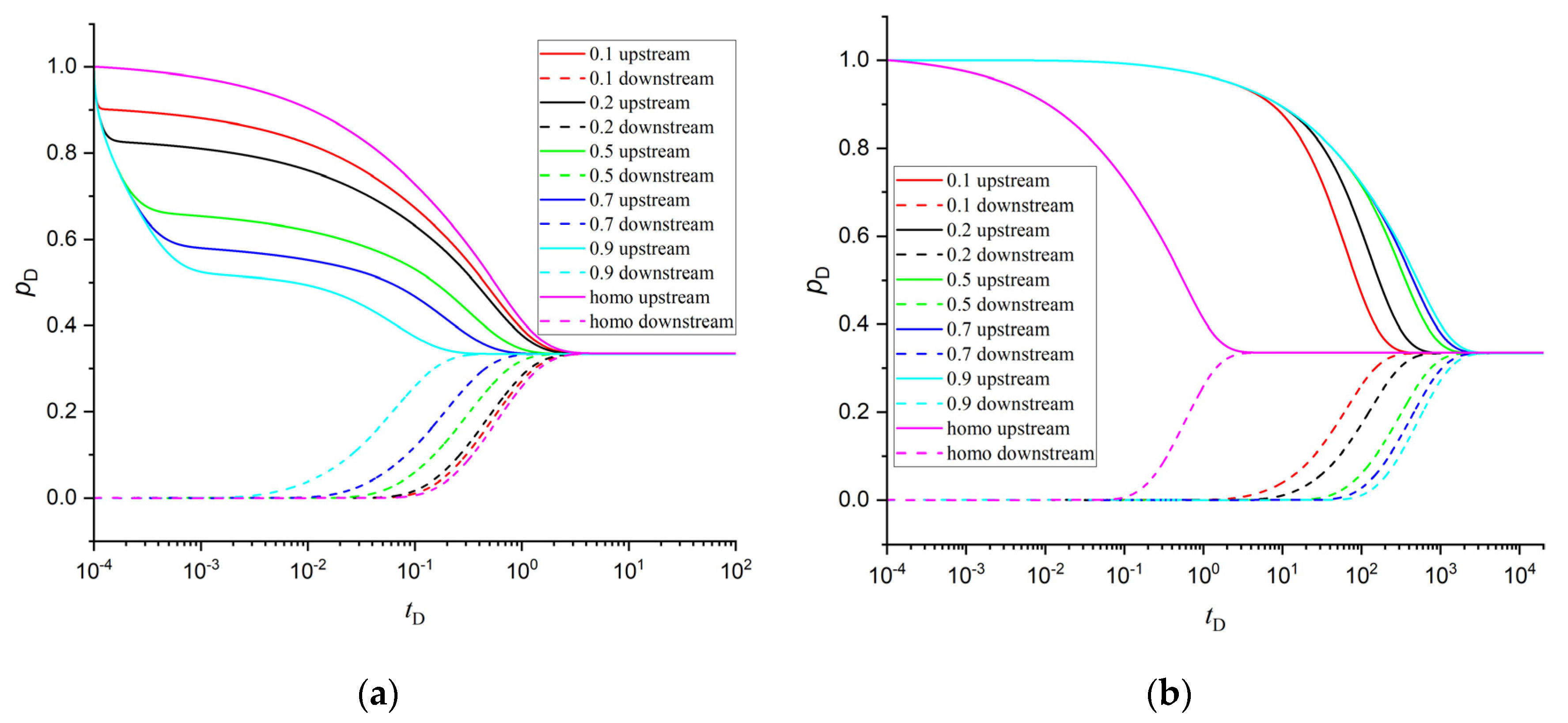
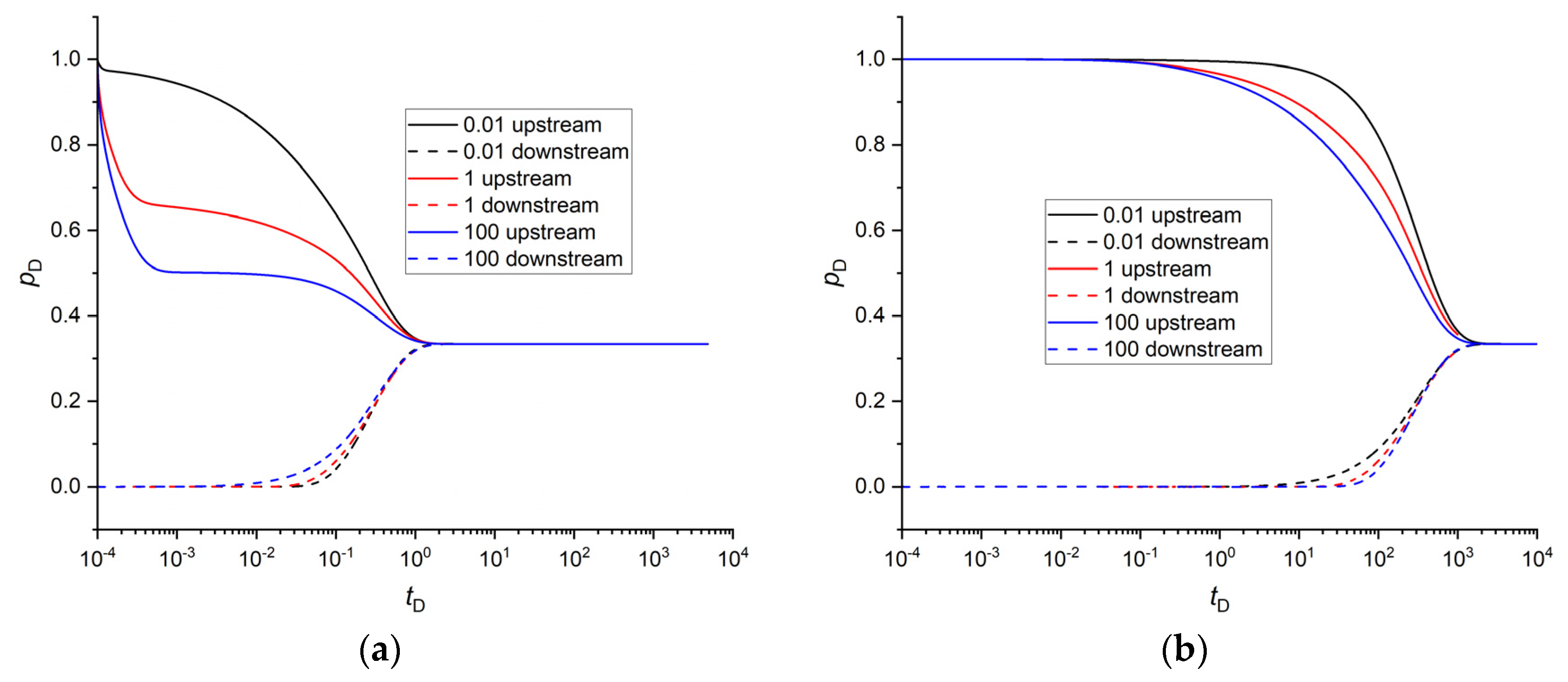
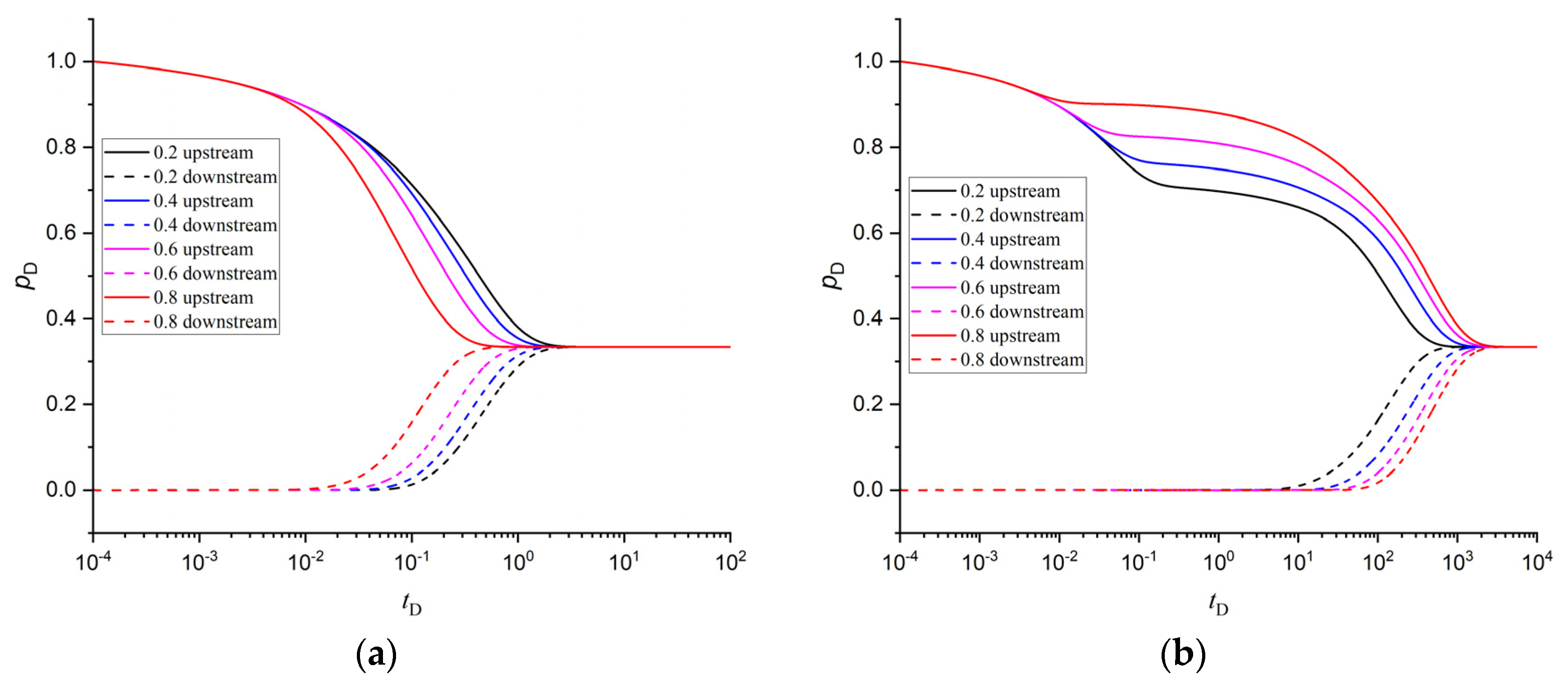
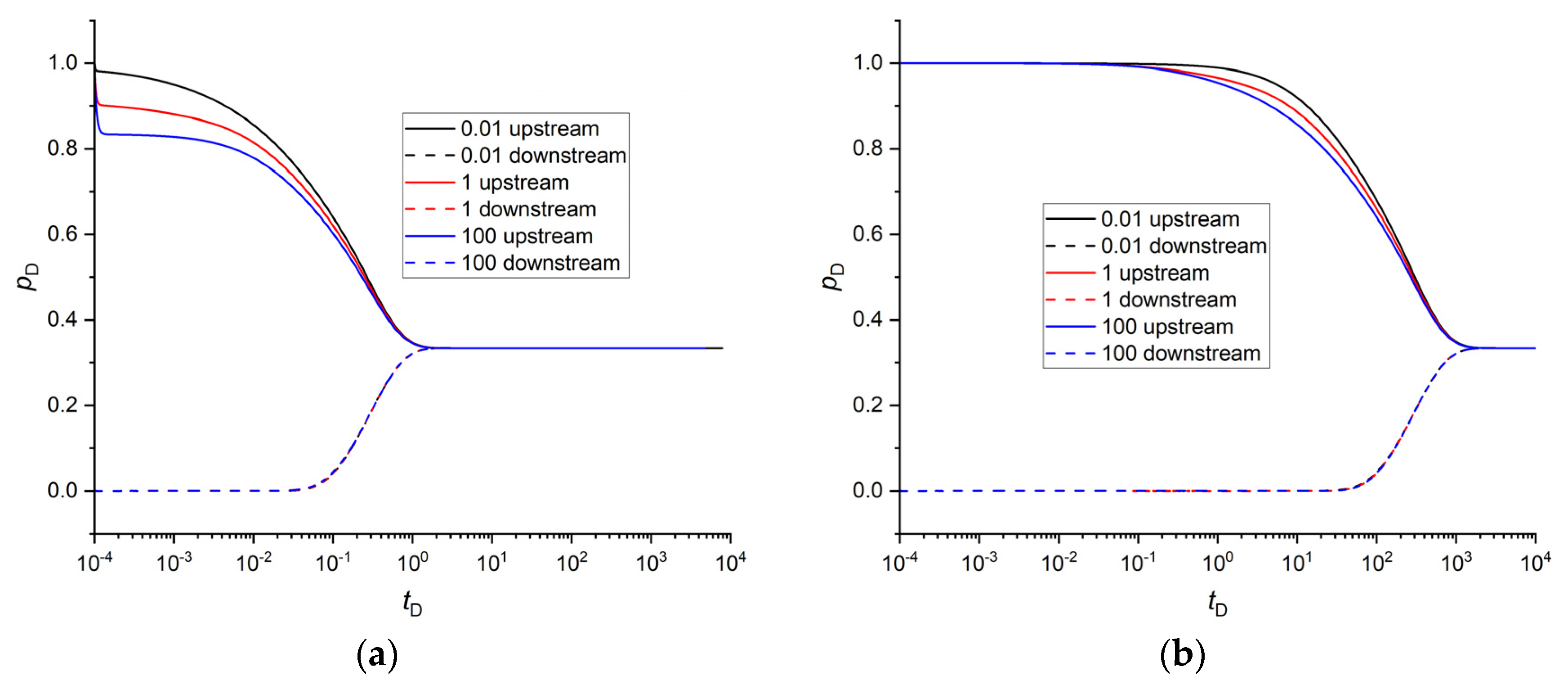
3.1. Pressure Curves of Two-Layer Cores

By using downstream parameters as the reference values and altering the upstream parameters, we can observe from Figure 4 that, although the thickness of two layers is different, the final dimensionless pressures are all balanced at 0.33. As, according to the gas equation of state, the final equilibrium pressure is determined by the storativity ratio. The shape of downstream pressures with different thicknesses and permeability ratios is similar to that of homogeneous cores. If the upstream permeability is larger than the downstream one (Figure 4a), the upstream pressure first drops rapidly and then tends to change in shape similar to that of a homogeneous core. The thicker the upstream layer compared to the downstream layer, the faster the pressure drops and the earlier the pressure equilibrium is reached. If the upstream permeability is smaller than the downstream one (Figure 4b), the upstream pressure shape is similar to that of a homogeneous core. Initially, the upstream pressures of all cores coincide. The thicker the upstream layer compared to the downstream layer, the slower the pressure drop and the later the pressure equilibrium is reached. The separation position of the upstream pressure curve reflects the thickness of the upstream layer because the early upstream pressure is mainly controlled by the permeability of the layer connected with the upstream and is not affected by the layer connect with the downstream.

Figure 5a depicts the pressure curves for two-layer cores with varying permeability ratios. If the upstream permeability is larger than the downstream one, the pressure in the beginning section decreases faster with the increase in the upstream permeability, but they almost simultaneously reach equilibrium. Conversely, if the upstream permeability is smaller than the downstream one, as the upstream permeability decreases, the drop in upstream pressure slows down, and equilibrium tends to be reached later. If testing is performed with the upstream and downstream directions reversed, there is a significant change in the shape of the pressure curves (Figure 5b). Initially, all upstream pressure curves coincide, but they begin to separate at approximately the same location. The is because when the upstream layer is used as a reference, its permeability is constant. The early upstream pressure is controlled by it. As the downstream permeability decreases, the pressure drop slows down, and the pressure reaches equilibrium later. If the downstream permeability is larger than the upstream one (permeability ratio > 1), the pressure curves almost coincide completely.

If the upstream permeability is larger than the downstream one (Figure 6a), as the storativity ratio increases, the early rapid decline section (for a permeability ratio of 100, t_D < 4 × 10⁻⁴) of the upstream pressure curve becomes longer and longer. This is because if the upstream storativity is larger than the downstream one, the increase in the pressure near the upstream is slower, and the large pressure difference between the upstream and the core can be maintained for a longer time. On the contrary, due to the smaller storativity, the core pressure near the downstream rises rapidly, resulting in a larger pressure difference between the core and the downstream. Therefore, the downstream pressure rises faster with the increase in the storativity ratio. If the upstream permeability is smaller than the downstream one, all pressure curves overlap in the early stage. Then, the upstream pressure drops faster, and the downstream pressure rises slower with the increase in the storativity ratio (Figure 6b). The storativity ratio does not affect the time in which the pressure reaches equilibrium.

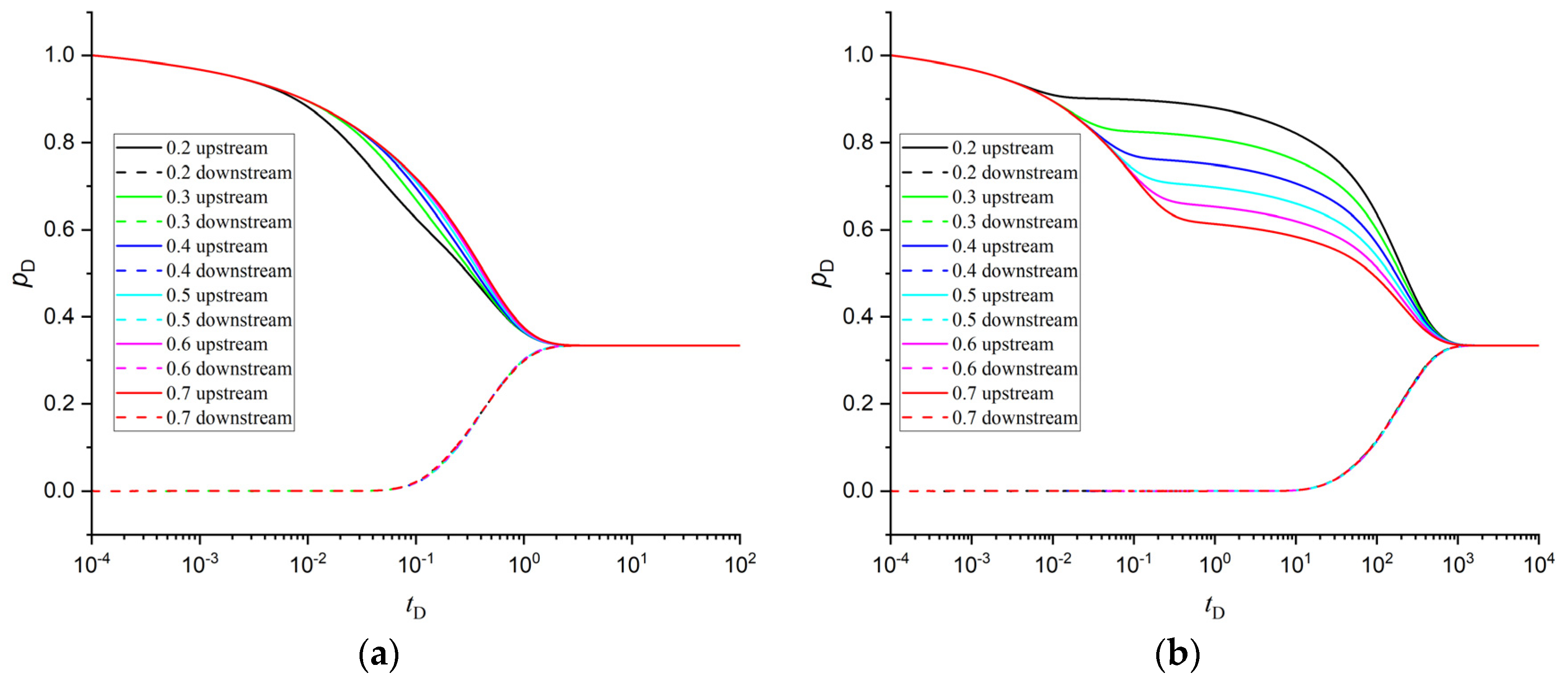
3.2. Pressure Curves of Three-Layer Cores

If the core is composed of three layers, the parameters of the upstream and downstream sides are equal and used as reference values, and the interlayer parameters are changed. The permeability ratio is the permeability of the interlayer to that of the two ends. The pressure shape of the downstream is similar to the homogeneous ones (Figure 7). As mentioned earlier, if the upstream layer is selected as the reference layer, its permeability remains unchanged. Upstream pressure coincides with the early stage. If the interlayer permeability is larger than that of two ends (Figure 7a), the shape of the upstream pressure is similar to that of a homogeneous one. As the thickness of the interlayer increases, the upstream pressure decreases faster, the downstream pressure rises faster, and the pressure equilibrium is reached earlier. If the interlayer permeability is smaller than that of two ends, compared with homogeneous cores, the upstream pressure begins to decrease rapidly, and then a slower pressure drop stage appears (Figure 7b). This is because the interlayer prevents the flow of fluid from upstream to downstream, slowing down the decrease in upstream pressure. With the increase in the interlayer thickness, the pressure drop becomes slow earlier, and the pressure reaches equilibrium later.

The downstream pressure and the time of pressure equilibrium are not affected by the location of the interlayer (Figure 8). If the interlayer permeability is larger than that of two ends (Figure 8a), as the interlayer is closer to the upstream, the upstream pressure begins to decrease earlier, but the time to equilibrium is not affected. If the distance of the interlayer to the upstream exceeds half of the length of the specimen, the upstream pressure is almost unaffected. If the upstream permeability is smaller than the interlayer one (Figure 8b), the drop of the upstream pressure slows down earlier as the interlayer approaches the upstream.

The permeability of the interlayer does not affect the separation location (t_D $\approx$ 6 × 10⁻²) of the upstream pressure curves (Figure 9). If the permeability of the interlayer is lower than that of the two ends, the upstream pressure decreases more slowly, and the pressure reaches equilibrium later. Otherwise, the upstream pressure decreases faster, and the pressure curve almost overlaps if the permeability ratio exceeds 10. This is because the core layers are connected in series, and, according to the law of series resistance, when the permeability difference is large, the equivalent behavior is controlled by the minimum permeability.

If the interlayer permeability is larger than that of the two ends (Figure 10a), the upstream pressure decreases at an increasing rate with the storativity ratio decrease. This is because, at this point, the fluid can flow faster through the interlayer. If the interlayer permeability is smaller than that of the two ends (Figure 10b), as the storativity of the interlayer decreases, the upstream pressure decreases faster. As the higher storativity ratio of the interlayer allows it to accommodate more fluid from upstream, the downstream pressure curve is not significantly affected by the storativity. The upstream and downstream pressure curves of different storativity ratios intersect when approaching equilibrium. The storativity ratio does not affect the time for pressure to reach equilibrium because the time of the fluid flow through the core is mainly controlled by the permeability.

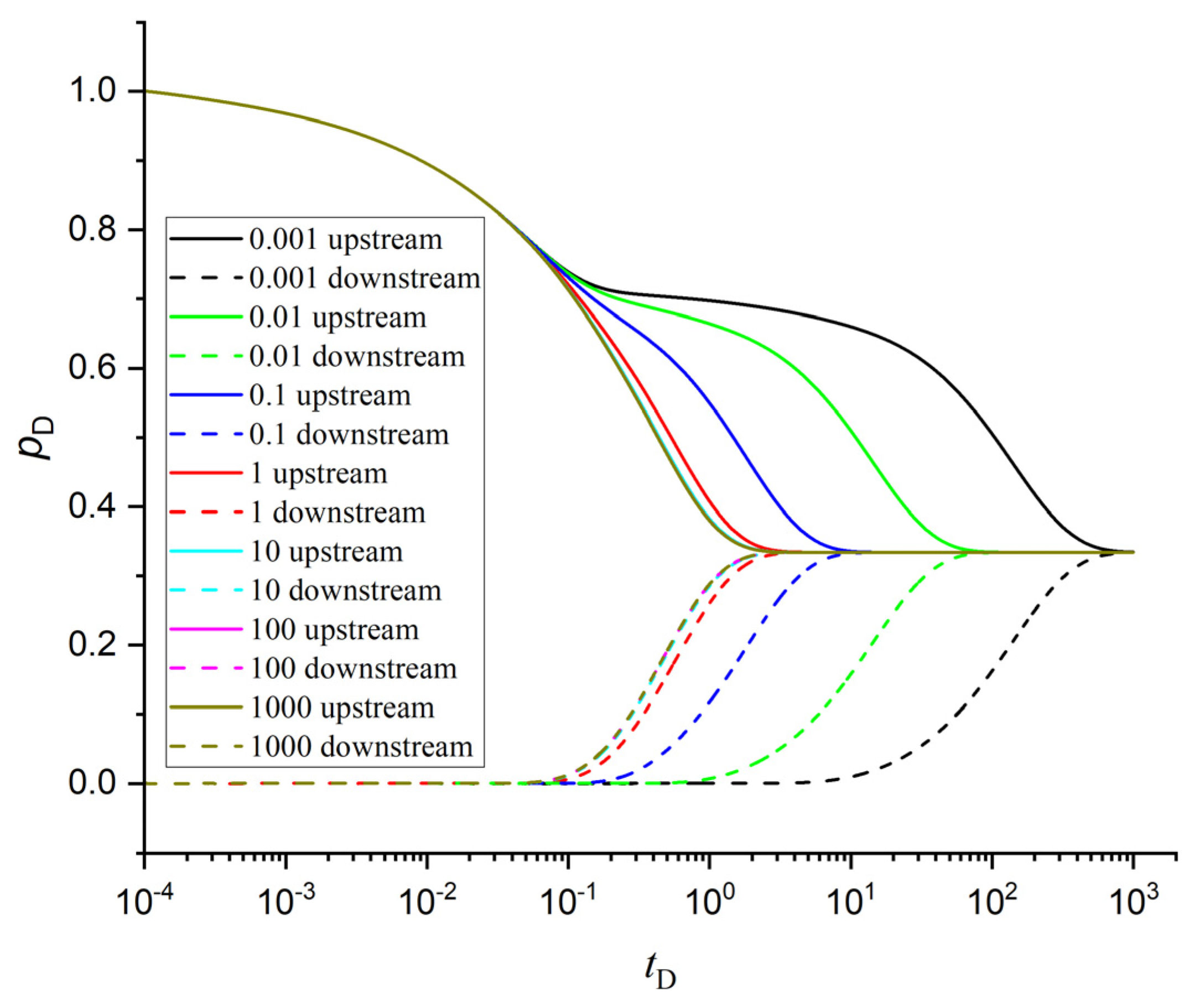
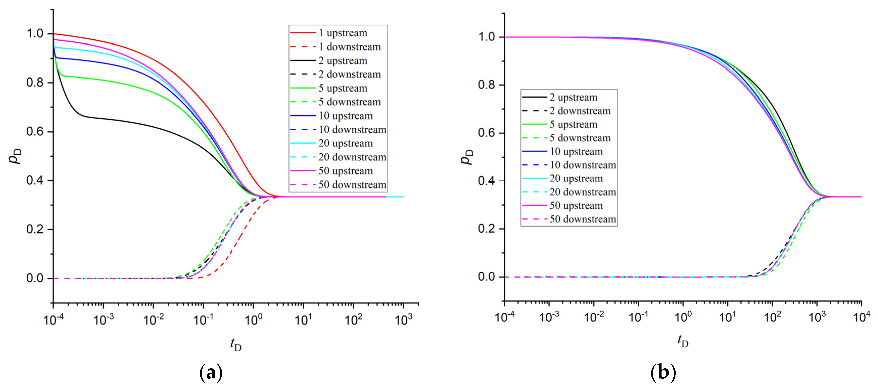
3.3. Pressure Curves of Multilayer Cores

A multilayer core consists of two alternating layers of different properties with equal thicknesses. For multilayer cores, the shape characteristics of the pressure curve under different parameters are similar to those of two-layer ones. As the upstream permeability decreases, the upstream pressure drop slows down, and the pressure reaches equilibrium later (Figure 11). If the permeability ratio is larger than 10, the pressure curves almost overlap. If the upstream permeability is larger than that of the next layer, a more rapid pressure drop segment exists on the upstream pressure curves compared to that of a homogeneous core. As the number of layers increases, this segment becomes shorter (Figure 12a). If the upstream permeability is lower than that of the next layer, and the number of layers exceeds 10, the upstream and downstream pressure curves almost overlap, respectively (Figure 12b). The impact of the storativity ratio on the pressure curve is similar to that of the two-layer cores (Figure 13). The difference is that if the number of layers is more than 10, the downstream pressure curves almost overlap.

4. Characteristics of Pressure Derivative Curves

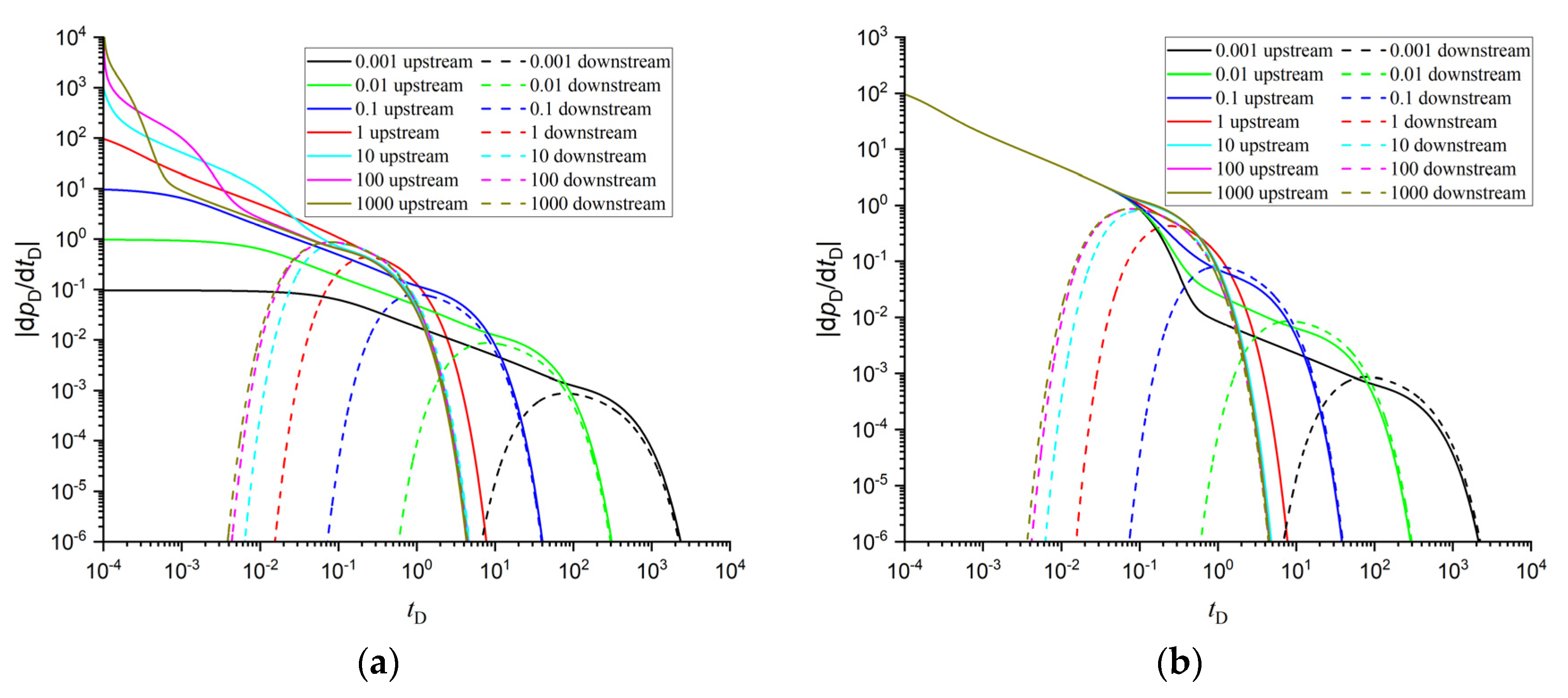
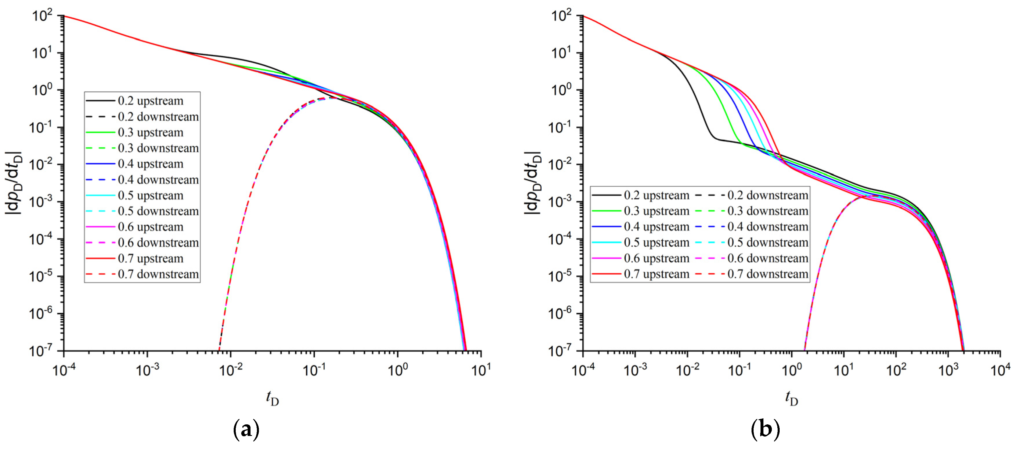
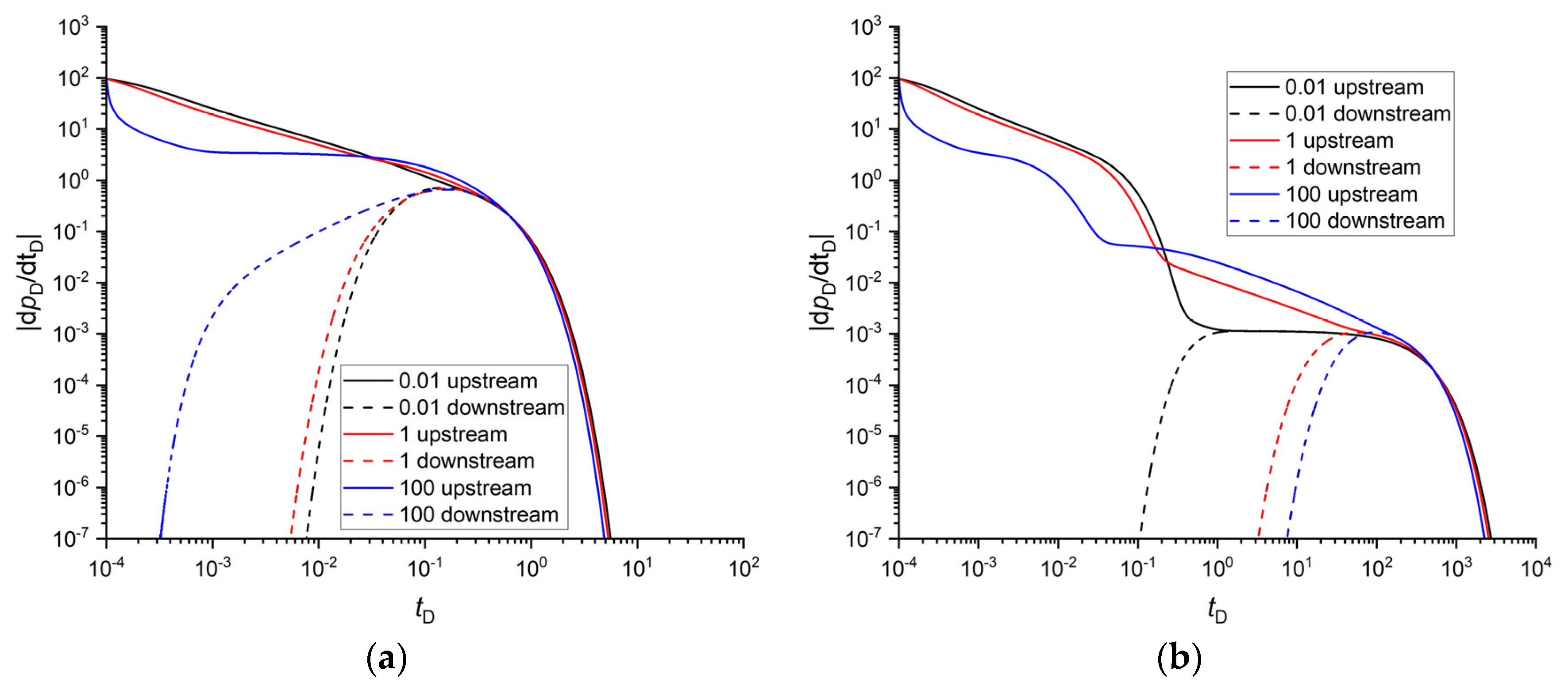
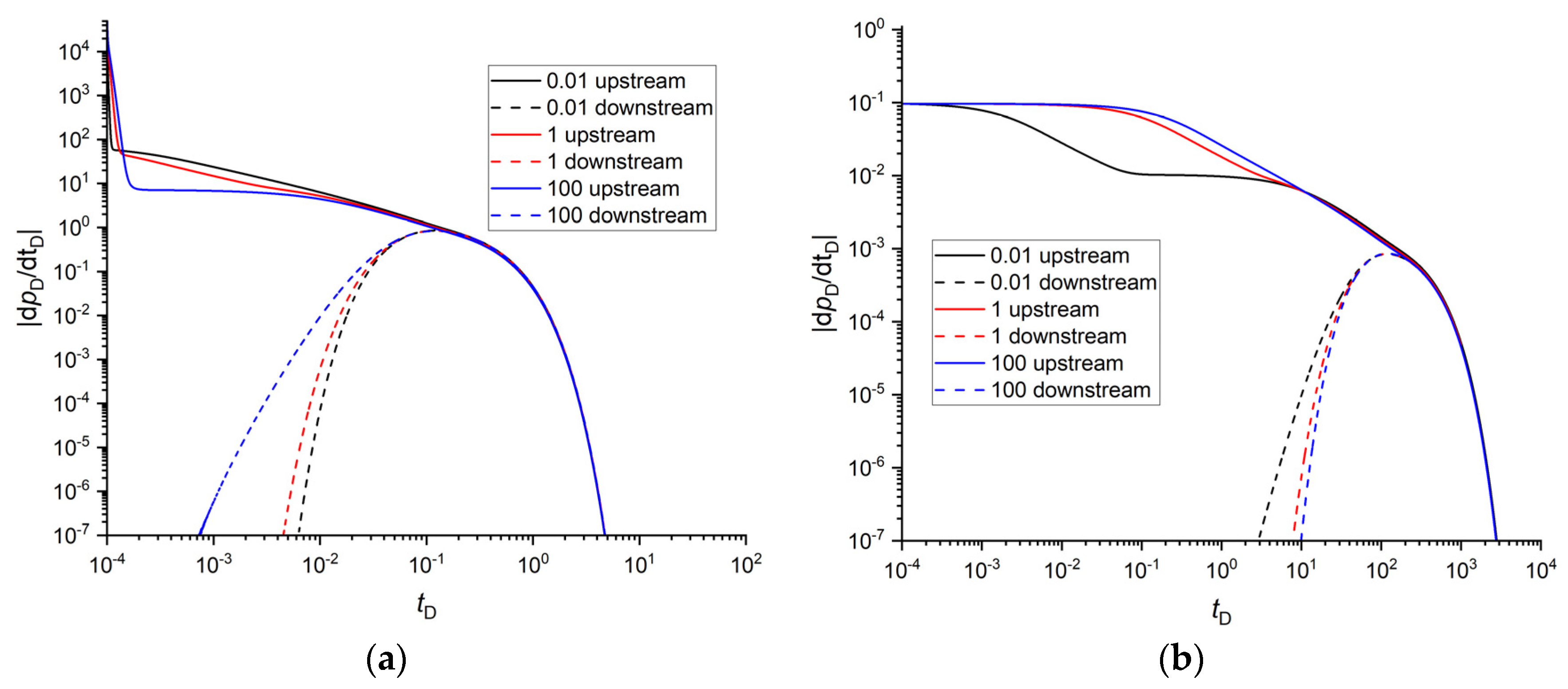
4.1. Pressure Derivative Curves of Two-Layer Cores

For two-layer cores with different permeabilities and equal thicknesses, if the upstream permeability is bigger than the downstream one, there are two parallel straight-line segments on the early pressure derivative curves (e.g., Figure 14a; permeability ratio of 100; the first straight-line segment: 2 × 10⁻⁴ < t_D < 5 × 10⁻⁴; the second straight-line segment 4 × 10⁻³ < t_D < 5 × 10⁻²). The inclined straight-line segments with different permeability ratios are parallel to each other. With the increase in the permeability ratio, the first straight-line segment becomes shorter, and the second straight-line segment becomes longer. If the upstream permeability is lower than the downstream one, there are both horizontal and inclined straight-line segments on the pressure derivative curves (e.g., Figure 14a: permeability ratio: 0.001; the horizontal straight-line segment: 10⁻⁴ < t_D < 2 × 10⁻²; the inclined straight-line segment: 0.2 < t_D < 100). The inclined straight-line segment of the pressure derivative with lower permeability is parallel to the straight-line segment of the pressure derivative with a larger permeability ratio. If the upstream and downstream are reversed (Figure 14b), at the beginning, the pressure derivatives are inclined straight-line segments that coincide (e.g., Figure 14b, 10⁻⁴ < t_D < 3 × 10⁻²). The separation point of the pressure derivative curves is not affected by the permeability ratio. If the upstream permeability is higher than the downstream one, a second straight-line segment parallel to the first one appears later (e.g., Figure 14b; permeability ratio: 0.001; 0.5 < t_D < 100). As the upstream permeability increases, the second straight-line segment becomes longer.

If the upstream permeability is higher than that of the downstream, as the thickness of the upstream layer increases, the first straight-line segments become shorter (Figure 15a). If the upstream thickness is less than half of the core length, it is difficult to distinguish the first straight-line segment. If the upstream permeability is lower than that of the downstream, as with the increase in the upstream thickness, the inclined straight-line segment becomes longer (Figure 15b).

If a larger permeability layer corresponds to a larger storativity layer, the pressure derivative curves exhibit horizontal straight-line segments that are parallel but separated for the upstream and downstream (e.g., Figure 16a, 10⁻³ < t_D < 10⁻¹). If this portion of the core is located upstream, it appears as a longer segment on a log-log plot. If the larger permeability and storativity are not at the same layer, pressure derivative curves for different storativity ratios appear as parallel inclined straight-line segments (e.g., Figure 16b, 0.4 < t_D < 100). If the permeability ratio is high, a higher storativity ratio leads to an earlier increase in the downstream pressure derivative (Figure 16a). Conversely, if the permeability ratio is low, a smaller storativity ratio leads to an earlier increase in the downstream pressure derivative (Figure 16b).

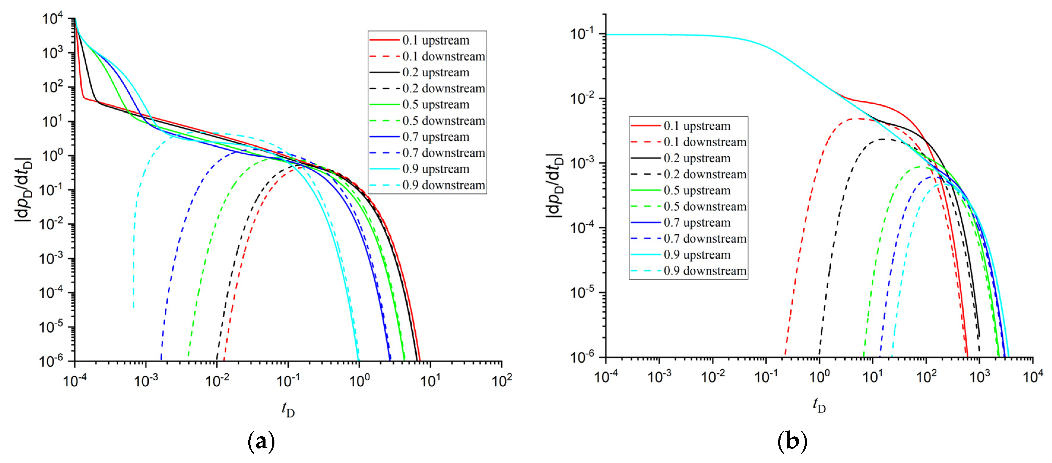
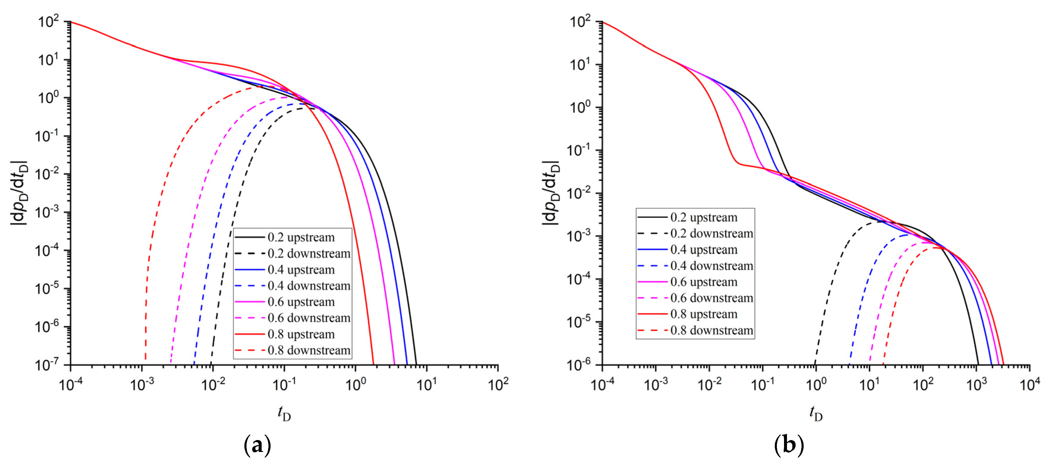
4.2. Pressure Derivative Curves of Three-Layer Cores

For three-layer cores, the upstream pressure derivative is unaffected by the interlayer location, permeability ratio, and interlayer thickness in the early period (Figure 17, Figure 18 and Figure 19). The upstream pressure derivative is an inclined straight-line segment in the early period. If the interlayer permeability is higher than that of the two ends, the upstream pressure derivative decrease slows down earlier with an increase in the interlayer thickness (Figure 17a). With the thickness of interlayer thinning, the upstream pressure derivative decreases slowly in the later period. If the interlayer permeability is lower than that of the two ends, there are two parallel straight-line segments on the upstream pressure derivative (e.g., Figure 17b, interlayer thickness 0.4, the first straight-line segment: 10⁻⁴ < t_D < 3 × 10⁻², the second straight-line segment: 0.2 < t_D < 100). The upstream pressure derivative has an accelerated decline segment (e.g., Figure 17b, interlayer thickness 0.8, 4 × 10⁻³ < t_D < 3 × 10⁻²). As the interlayer thickens and the distance to the upstream decreases, the transition from the first straight-line segment to the second straight-line segment occurs earlier (Figure 17b and Figure 18b). As the interlayer thickens and permeability decreases, the upstream pressure derivative decreases faster in the later period (Figure 17b and Figure 19).

The downstream pressure derivative curves for different interlayer locations overlap (Figure 18). As the interlayer permeability decreases, the downstream pressure derivative rises later (Figure 19). If the permeability ratio is greater than 10, the downstream pressure derivative is almost unaffected by the interlayer permeability. The pressure derivatives for different interlayer locations almost overlap during the late period (Figure 18). The interlayer permeability does not affect the transition location of the upstream pressure derivative from the first straight-line segment to the second straight-line segment (Figure 19).

If the interlayer permeability and storativity are all greater or smaller than those on both sides, a horizontal plateau appears on the pressure derivative curve (e.g., Figure 20b, 10 < t_D < 10²). Unlike two-layer cores, if the interlayer storativity is larger than that of the two sides, only the upstream plateau appears (Figure 20a); if the interlayer storativity is smaller that of the two sides, the upstream and downstream plateau overlap at later times (Figure 20b). If the permeability ratio is relatively high, as the storativity ratio increases, the downstream pressure derivative rises earlier (Figure 20a). If the permeability is relatively small, as the storativity ratio decreases, the downstream pressure derivative rises earlier (Figure 20b).

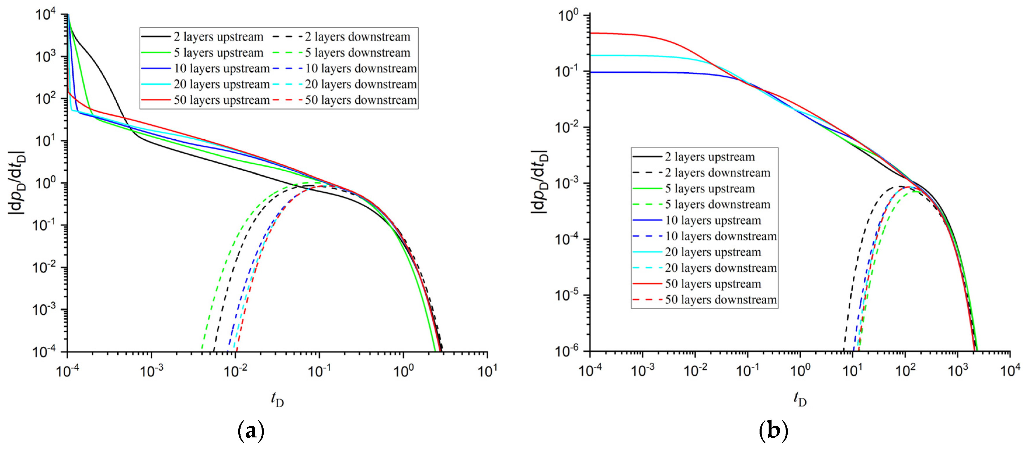
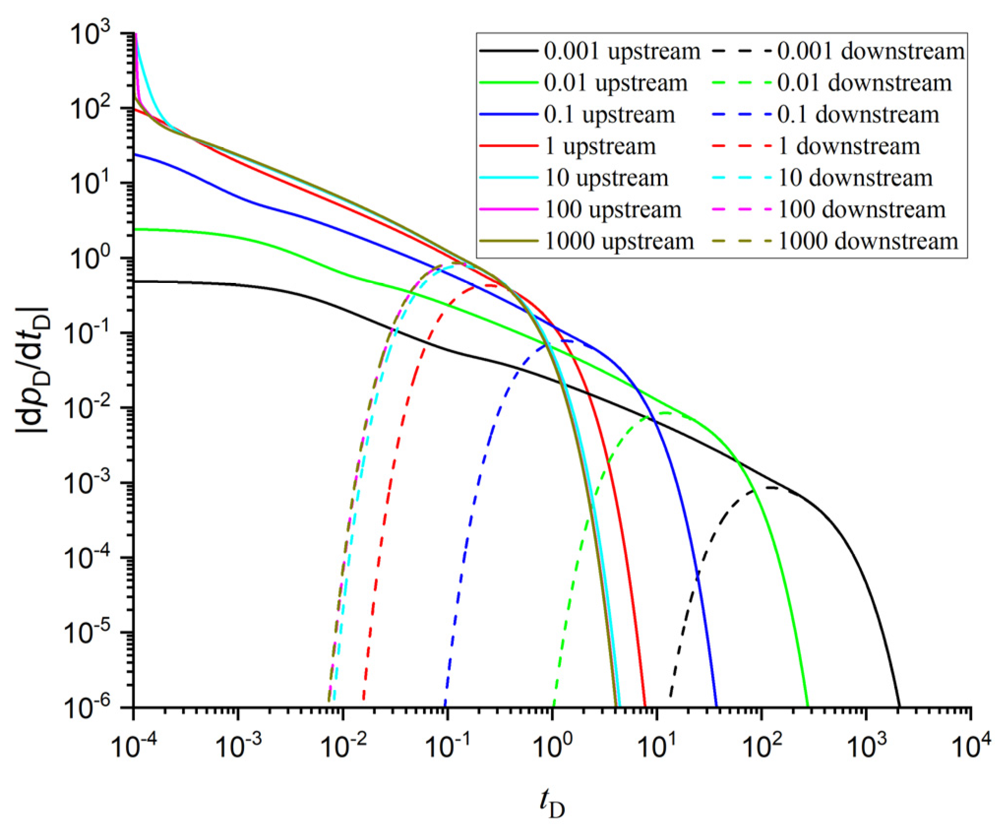
4.3. Pressure Derivative Curves of Multilayer Cores

If the upstream permeability is higher than that of the next layer, the first straight-line segment of the pressure derivative becomes shorter with the increase in the layer number, and the value of the second straight-line segment becomes greater (Figure 21a). Unlike two-layer cores, the straight-line segment is not particularly straight. If the upstream permeability is lower than that of the next layer, the horizontal straight-line segment becomes shorter with the increase in the layer number, but the pressure derivative value increases. If the layer number does not exceed 10, the horizontal straight-line segment of the pressure derivative coincides with this (Figure 21b). For multilayer cores, the influences of the permeability and storativity ratio on the pressure derivative curve are similar to those of two-layer ones, except that the horizontal straight-line segment for multilayer cores is shorter (Figure 22 and Figure 23).

5. Permeability of Layered Cores

The core consists of two different permeability layers, k₁ and k₂, and α is the ratio of thickness of permeability k₁ layer to the core length. If the pressure difference at both ends remains constant in steady-state flow, the equivalent permeability for two different permeability layers in series is

$$k_{\mathrm{e}}=\frac{1}{\frac{\alpha }{k_1}+\frac{1-\alpha }{k_2}}$$

(17)

For homogeneous cores, the upstream and downstream pressure difference follows the following equation at the later stage of the pulse decay test [9]:

$$\ln \left(\Delta p_{\mathrm{D}}\right)=\ln \left(f_0\right)-m{t}_D$$

(18)

where Δp_D is the dimensionless pressure difference between upstream and downstream; t_D is the dimensionless time (refer to the Appendix A for specific definitions); and f₀ and m are constants related to vessel parameters, core parameters, and fluid compressibility. Equation (11) for the ln(Δp_D)~t_D coordinate is a straight line. For layered cores, a straight-line segment can also be found on ln(Δp_D)~t_D plot. Therefore, the tested permeability k_t of layered cores can be obtained by analyzing the simulated pressure data with this equation. The permeability error for pulse decay test is defined as follows:

$$Eor=\frac{k_{\mathrm{t}}-k_{\mathrm{e}}}{k_{\mathrm{e}}}\times 100\%$$

(19)

There may be some operational errors due to different data segments being analyzed. The data that best satisfy the semi-logarithmic straight-line segment were selected in the simulated data for analysis, ensuring the consistency of the obtained permeability.

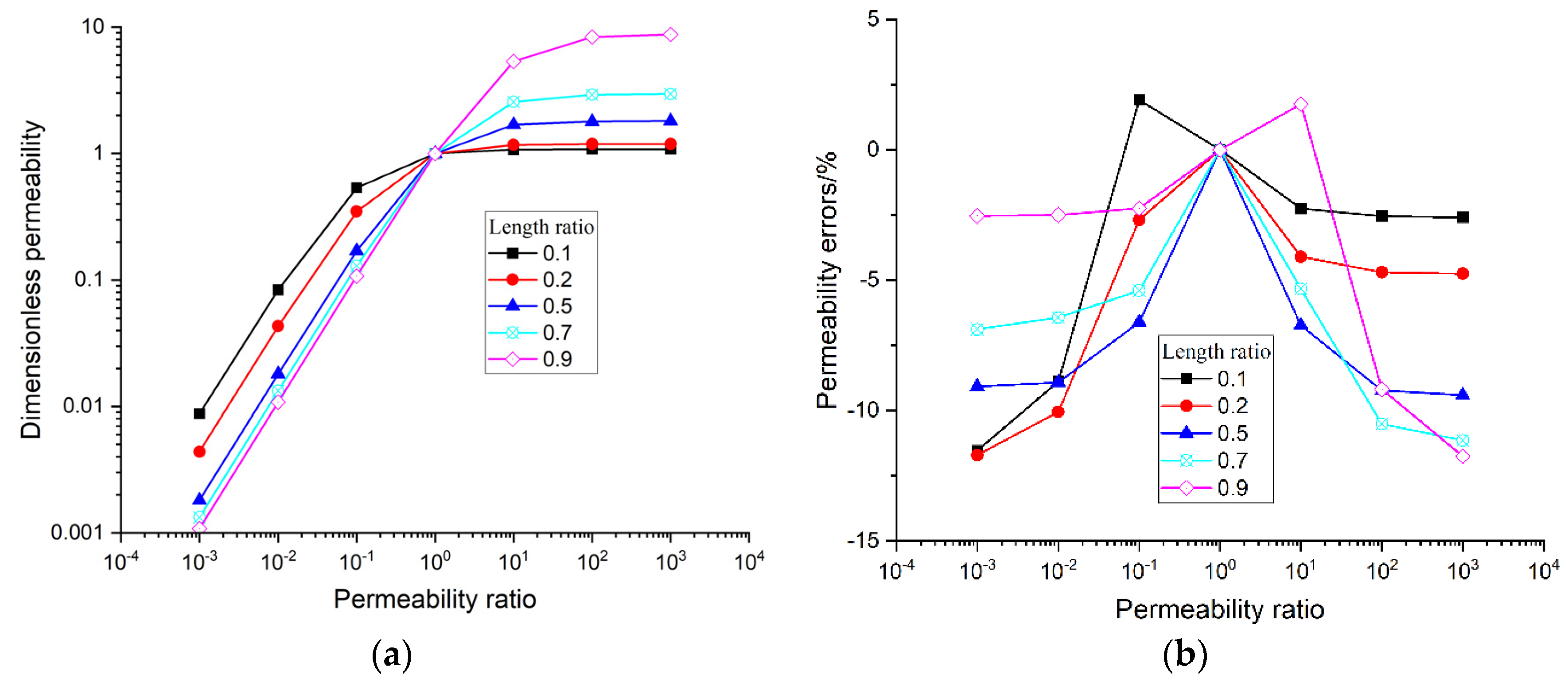
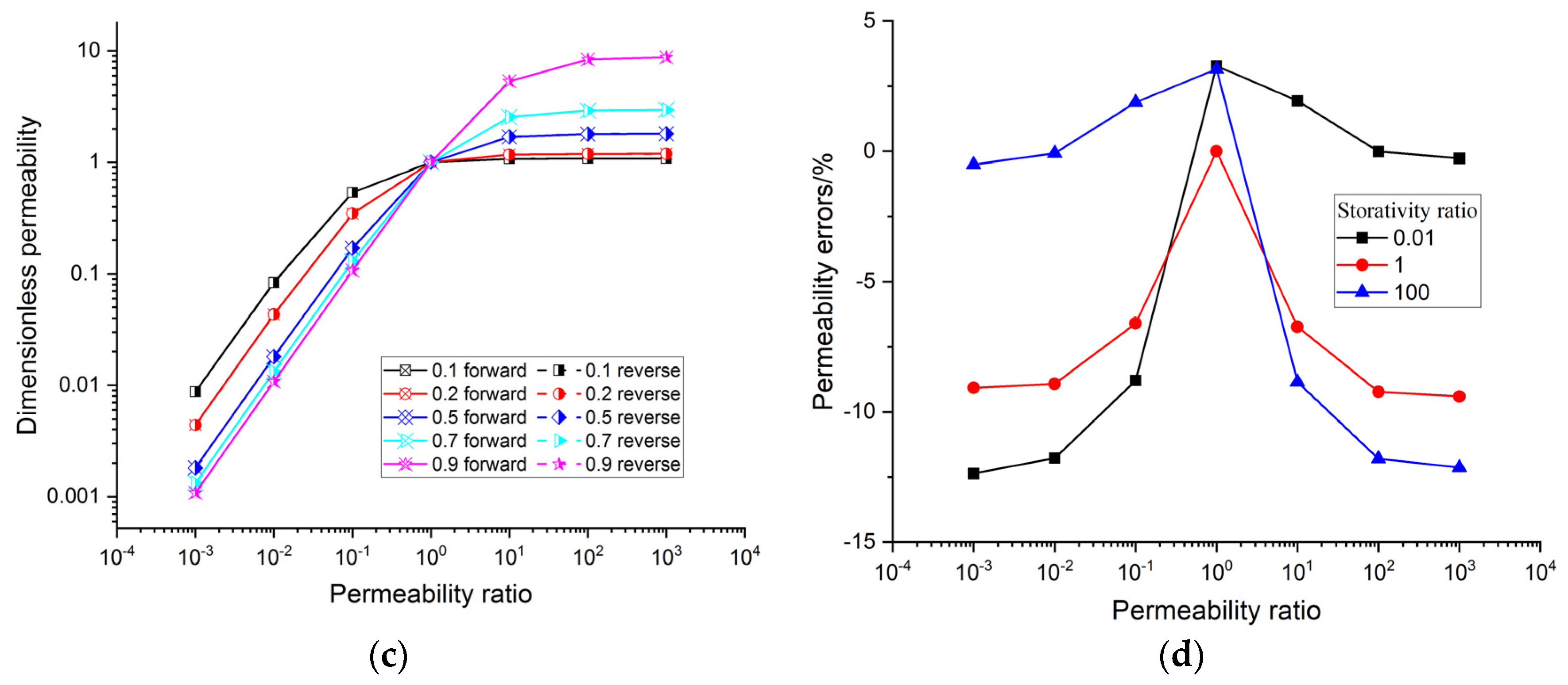
5.1. Permeability of Two-Layer Cores

If the core is composed of two layers, the error of the permeability tested using the pulse decay method to the equivalent permeability is shown in Figure 24. The tested permeability increases with the increase in permeability ratio. If the permeability ratio is greater than 100, the tested permeability remains basically unchanged. If the permeability ratio is less than 0.1, the tested permeability of the core generally increases linearly with the permeability ratio (Figure 24a). If the permeability ratio is less than 1, the test permeability decreases with the increase in the proportion of the upstream layer in the length. Otherwise, the tested permeability increases with the increase in the proportion of the upstream layer in the length. If the permeability ratio does not exceed three orders of magnitude, the error between the tested permeability and the equivalent permeability is within 12% (Figure 24b). In general, the error increases with the increase in the permeability difference between the two layers. As the thickness difference between the two layers decreases, the maximum error also decreases. For pulse decay tests, changing the upstream and downstream positions does not affect the tested permeability of layered cores (Figure 24c).

If the permeability ratio is 10⁻³, compared with homogeneous storativity, a storage ratio of 0.01 may cause an increase in permeability error of 3.3%, whereas a storage ratio of 100 may lead to a decrease in permeability error of 8.5%. If the permeability ratio is 10³, a storage ratio of 0.01 results in a decrease in permeability error of 9.1%, whereas a storage ratio of 100 leads to an increase in the permeability error of 2.7% (Figure 24d).

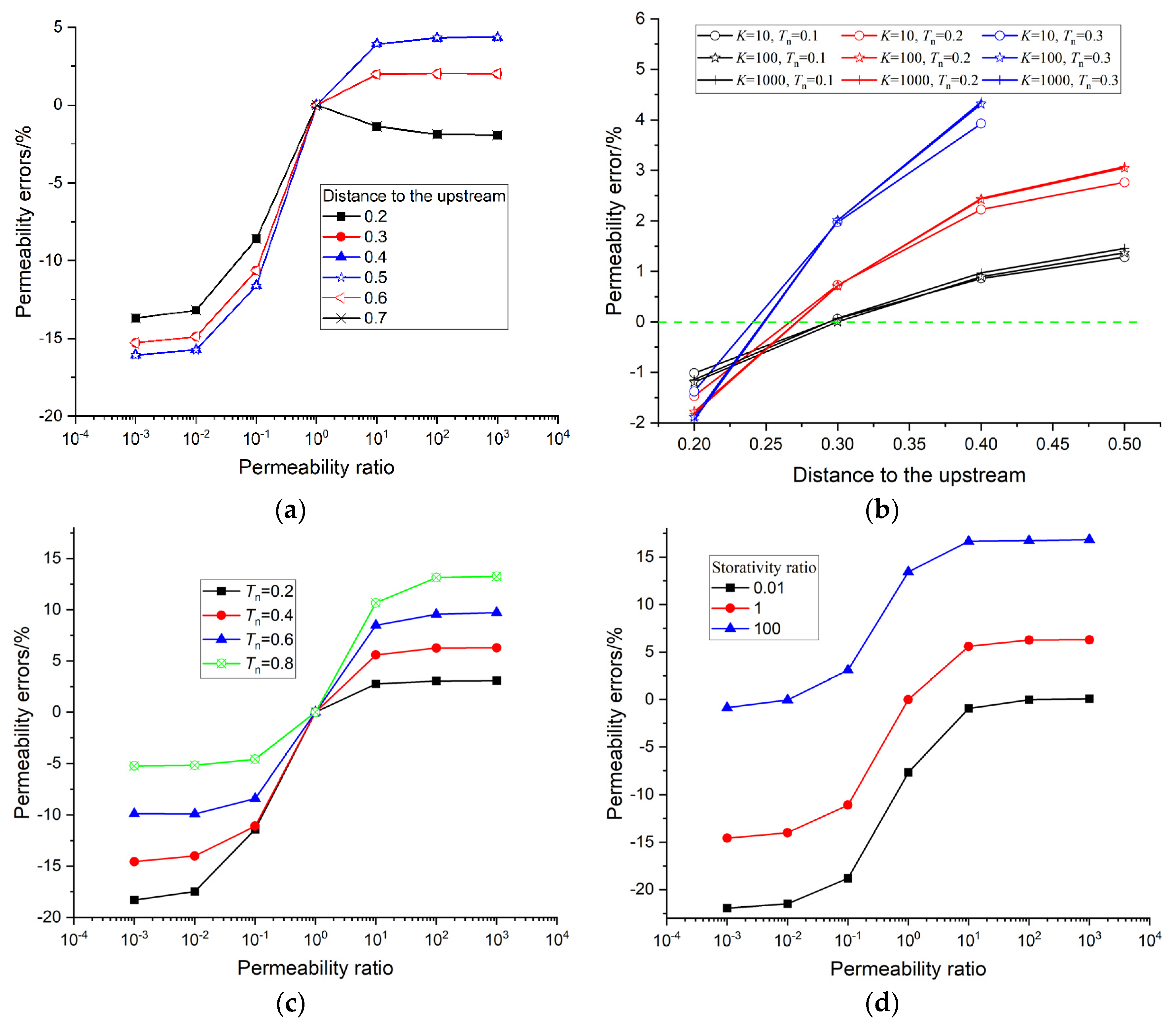
5.2. Permeability of Three-Layer Cores

The permeability and permeability error of three-layer cores are shown in Figure 25. The location of the interlayer has little impact on the permeability. Consistent with the conclusions for two-layer cores, if the interlayer is in the symmetric location of the upstream and downstream, the tested permeabilities are the same (Figure 25a). If the permeability ratio does not exceed three orders of magnitude, the difference between the permeability obtained from the pulse decay test and the equivalent model is within the range of 20% (Figure 25b). If the interlayer is at an appropriate location, the permeability obtained by the pulse decay test may be consistent with the equivalent permeability (Figure 25b, green line). When the thickness of the interlayer is 0.1, 0.2, and 0.3, these locations are approximately 0.3, 0.27, and 0.24, respectively.

As the difference in permeability between the interlayer and the two ends increases, the error in permeability increases. If the permeability difference between the interlayer and the two ends is over two orders of magnitude, the permeability error remains basically unchanged (Figure 25c). If the permeability ratio is less than 1, the permeability error decreases with the increase in interlayer thickness. Otherwise, the relationship between the permeability error and the interlayer thickness is opposite. The maximum permeability error is approximately 18%.

If the storativity between the interlayer and the two ends differs by two orders of magnitude, the tested permeability error may reach 22% (Figure 25d). Compared to cores with homogeneous storativity, if the permeability ratio is relatively small, an increase in the storativity ratio may lead to a 7.5% increase in permeability error; a large storativity ratio may lead to a decrease of 13.7% in permeability error. If the permeability ratio is relatively high, an increase in the storativity ratio may reduce the permeability error by 6.1%, and a decrease in the storativity ratio may increase the permeability error by 10.6%.

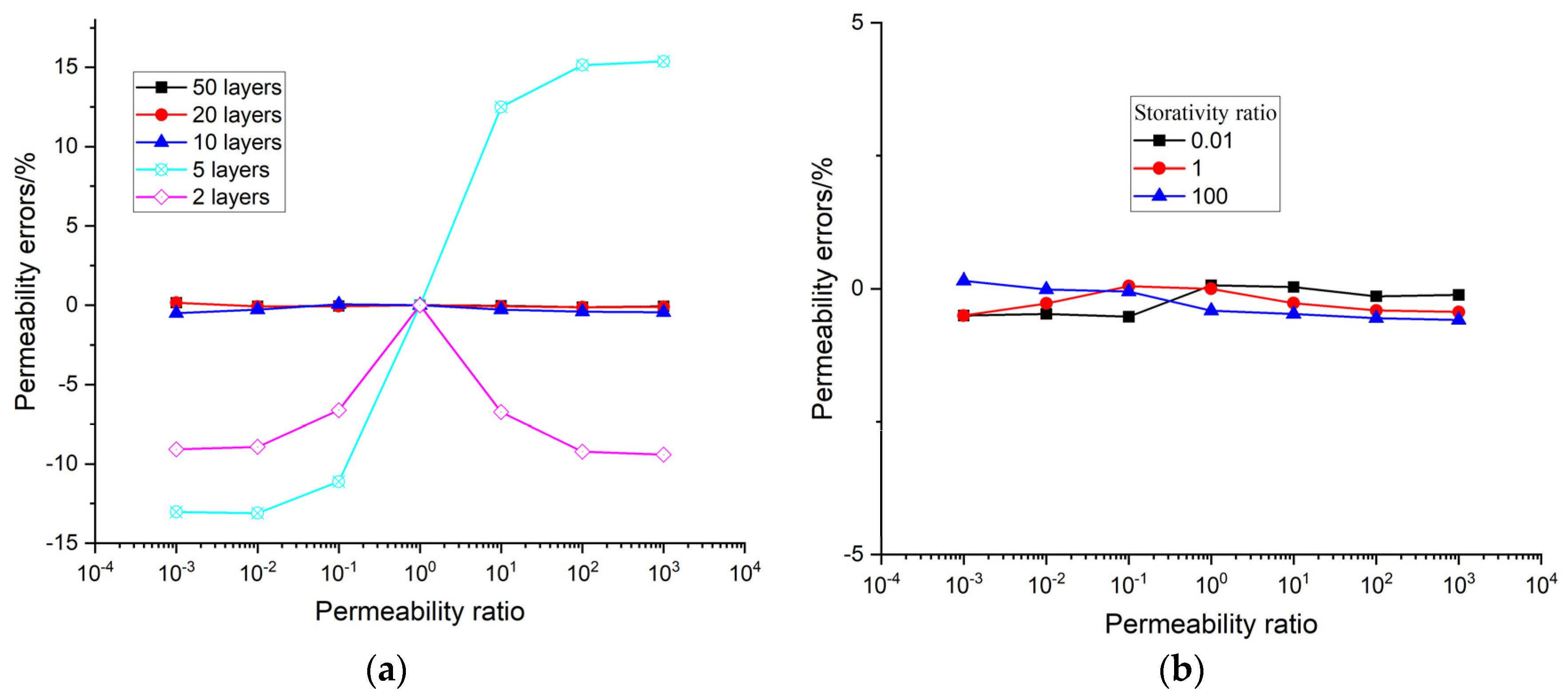
5.3. Permeability of Multilayer Cores

If the layer number is not less than 10, the permeability obtained from the pulse decay test is basically equal and consistent with the results of the equivalent model (Figure 26a). If the layer number is 2 or 5, there is a slight difference in permeability compared to the equivalent model. The maximum permeability error is less than 10% and 15.4% for two-layer and five-layer cores, respectively. If the layer number reaches 10, the difference in storativity within two orders of magnitude has little effect on the tested permeability (Figure 26b).

6. Conclusions

There is still a lack of comprehensive research on the influence of the layered structure of rock cores perpendicular to the flow direction during pulse decay testing. To determine the performance of pulse decay testing in layered rock cores, this study utilized numerical simulation to analyze the effects of the interlayer permeability ratio, storativity ratio, layer thickness, interlayer location, and layer number on the shape of pressure and pressure derivative curves. The tested permeability was compared with an equivalent permeability model. The applicability of pulse decay testing for layered cores was determined, and several valuable results were yielded.

For layered cores, if the upstream permeability is higher than that of the next layer, the upstream pressure curve initially has a rapid decline segment compared to that of homogeneous cores. This feature becomes less pronounced as the layer number increases and the upstream storativity decreases. Conversely, if the upstream permeability is lower than that of the next layer, the shape of the pressure curve is similar to that of a homogeneous core. Although the shape of the upstream pressure and pressure derivative curves is affected by the switching of the upstream and downstream, the tested permeability is not affected. The pressure derivative curve of layered cores has more inclined or horizontal straight-line segments than that of homogeneous cores. If the permeability distribution of the core is in the same order as the storativity, horizontal straight lines may appear on the pressure derivative curve. This feature weakens with the increase in the layer number, the increase in the permeability difference between layers, and the mismatch between the permeability and storativity. The permeability of the layered core examined using pulse decay testing is not completely consistent with the equivalent permeability, with a maximum error of up to 22%. This error is influenced by factors such as the ratio of interlayer permeability, storativity ratio, layer thickness, interlayer location, and layer number. If the layer number reaches 10 or more, the permeability obtained from the test is essentially equal to the equivalent permeability. To improve the accuracy of permeability analysis for a layered core, the characteristics of the pressure derivative curve can be used to analyze the test data through the curve fitting method.

In this study, the characteristics of pulse decay testing for layered cores were analyzed using only numerical simulation. In the future, pulse decay tests of layered cores will be carried out to verify the conclusions of this study. This study is only based on the linear Darcy flow governing equation. When the applied pressure pulse is large, it is necessary to consider the pressure-dependent permeability; when the average pressure is low, the gas slippage effect cannot be ignored; when CH₄ or CO₂ is used as the testing fluid, it is often necessary to take the gas adsorption effect into account. At these points, the flow governing equation is nonlinear, and their impacts on the performance on the pulse decay test of layered rock cores need further research.

References

1. Mansouri, M.; Parhiz, M.; Bayati, B.; Ahmadi, Y. Preparation of Nickel Oxide Supported Zeolite Catalyst (NiO/Na-ZSm-5) for Asphaltene Adsorption: A Kinetic and Thermodynamic Study. Iran. J. Oil Gas Sci. Technol. 2021, 10, 63–89. [Google Scholar]
2. Ahmadi, Y.; Aminshahidy, B. Inhibition of asphaltene precipitation by hydrophobic CaO and SiO2 nanoparticles during natural depletion and CO2 tests. Int. J. Oil Gas Coal Technol. 2020, 24, 394–414. [Google Scholar] [CrossRef]
3. Feng, R.; Pandey, R. Investigation of various pressure transient techniques on permeability measurement of unconventional gas reservoirs. Transp. Porous Media 2017, 120, 495–514. [Google Scholar] [CrossRef]
4. Song, F.; Bo, L.; Zhang, S.; Sun, Y. Nonlinear flow in low permeability reservoirs: Modelling and experimental verification. Adv. Geo-Energy Res. 2019, 3, 76–81. [Google Scholar] [CrossRef]
5. Han, G.; Liu, X.; Huang, J. Theoretical Comparison of Test Performance of Different Pulse Decay Methods for Unconventional Cores. Energies 2020, 13, 4557. [Google Scholar] [CrossRef]
6. Ghanizadeh, A.; Gasparik, M.; Amann-Hildenbrand, A.; Gensterblum, Y.; Krooss, B.M. Experimental study of fluid transport processes in the matrix system of the European organic-rich shales: I. Scandinavian Alum Shale. Mar. Pet. Geol. 2014, 51, 79–99. [Google Scholar] [CrossRef]
7. Brace, W.F.; Walsh, J.B.; Frangos, W.T. Permeability of granite under high pressure. J. Geophys. Res. 1968, 73, 2225–2236. [Google Scholar] [CrossRef]
8. Hsieh, P.A.; Tracy, J.V.; Neuzil, C.E.; Bredehoeft, J.D.; Silliman, S.E. A transient laboratory method for determining the hydraulic properties of ‘tight’ rocks-I. Theory. Int. J. Rock Mech. Min. Sci. Geomech. Abstr. 1981, 18, 245–252. [Google Scholar] [CrossRef]
9. Jones, S.C. A technique for faster pulse-decay permeability measurements in tight rocks. SPE Eval. Form 1997, 12, 19–25. [Google Scholar] [CrossRef]
10. Wang, Y.; Nolte, S.; Tian, Z.; Amann-Hildenbrand, A.; Krooss, B.; Wang, M. A modified pulse-decay approach to simultaneously measure permeability and porosity of tight rocks. Energy Sci. Eng. 2021, 9, 2354–2363. [Google Scholar] [CrossRef]
11. Zhao, Y.; Wang, C.; Zhang, Y.; Liu, Q. A Method of Differentiating the Early-Time and Late-Time Behavior in Pressure-Pulse Decay Permeametry. Geofluids 2019, 2019, 1309042. [Google Scholar] [CrossRef]
12. Wang, Y.; Nolte, S.; Gaus, G.; Tian, Z.; Amann-Hildenbrand, A.; Krooss, B.; Wang, M. An Early-Time Solution of Pulse-Decay Method for Permeability Measurement of Tight Rocks. J. Geophys. Res. Solid Earth 2021, 126, e2021JB022422. [Google Scholar] [CrossRef]
13. Wang, Y.; Tian, Z.; Nolte, S.; Krooss, B.; Wang, M. An improved straight-line method for permeability and porosity determination for tight reservoirs using pulse-decay measurements. J. Nat. Gas Sci. Eng. 2022, 105, 104708. [Google Scholar] [CrossRef]
14. Zhao, Y.; Zhang, K.; Wang, C.; Bi, J. A large pressure pulse decay method to simultaneously measure permeability and compressibility of tight rocks. J. Nat. Gas Sci. Eng. 2022, 98, 104395. [Google Scholar] [CrossRef]
15. Wang, Y.; Tian, Z.; Nolte, S.; Krooss, B.; Wang, M. Infuence of Equation Nonlinearity on Pulse-Decay Permeability Measurements of Tight Porous Media. Transp. Porous Media 2023, 148, 291–315. [Google Scholar] [CrossRef]
16. Tian, Z.; Zhang, D.; Wang, Y.; Zhou, G.; Zhang, S.; Wang, M. Inertial solution for high-pressure-difference pulse-decay measurement through microporous media. J. Fluid Mech. 2023, 971, R1. [Google Scholar] [CrossRef]
17. Aljamaan, H.; Ismail, M.A.; Kovscek, A.R. Experimental investigation and Grand Canonical Monte Carlo simulation of gas shale adsorption from the macro to the nano scale. J. Nat. Gas Sci. Eng. 2017, 48, 119–137. [Google Scholar] [CrossRef]
18. Cui, X.; Bustion, A.M.M.; Bustion, R.M. Measurements of gas permeability and diffusivity of tight reservoir rocks: Different approaches and their applications. Geofluids 2009, 9, 208–223. [Google Scholar] [CrossRef]
19. Han, G.; Chen, Y.; Liu, X. Investigation of Analysis Methods for Pulse Decay Tests Considering Gas Adsorption. Energies 2019, 12, 2562. [Google Scholar] [CrossRef]
20. Chen, H.; Liu, H.H. Pressure pulse-decay tests in a dual-continuum medium: An improved technique to estimate flow parameters. J. Nat. Gas Sci. Eng. 2019, 65, 16–24. [Google Scholar] [CrossRef]
21. Liu, H.; Lai, B.; Chen, J.; Georgi, D. Pressure pulse-decay tests in a dual-continuum medium: Late-time behavior. J. Petrol. Sci. Eng. 2016, 147, 292–301. [Google Scholar]
22. Jia, B.; Tsau, J.; Barati, R. Experimental and numerical investigations of permeability in heterogeneous fractured tight porous media. J. Nat. Gas Sci. Eng. 2018, 58, 216–233. [Google Scholar] [CrossRef]
23. Jia, B.; Tsau, J.; Barati, R.; Zhang, F. Impact of Heterogeneity on the transient gas flow process in tight rock. Energies 2019, 12, 3559. [Google Scholar] [CrossRef]
24. Alnoaimi, K.R.; Duchateau, C.; Kovscek, A.R. Characterization and measurement of multiscale gas transport in shale-core samples. SPE J. 2016, 21, 573–588. [Google Scholar] [CrossRef]
25. Alnoaimi, K.R.; Kovscek, A.R. Influence of microcracks on flow and storage capacities of gas shales at core scale. Transp. Porous Med. 2019, 127, 53–84. [Google Scholar] [CrossRef]
26. Cronin, M.B.; Flemings, P.B.; Bhandari, A.R. Dual-permeability microstratigraphy in the Barnett Shale. J. Pet. Sci. Eng. 2016, 142, 119–128. [Google Scholar] [CrossRef]
27. Bhandari, A.R.; Flemings, P.B.; Polito, P.J.; Cronin, M.B.; Bryant, S.L. Anisotropy and Stress Dependence of Permeability in the Barnett Shale. Transp. Porous Med. 2015, 108, 393–411. [Google Scholar] [CrossRef]
28. Cronin, M.B. Core-Scale Heterogeneity and Dual-Permeability Pore Structure in the Barnett Shale. Ph.D. Thesis, The University of Texas at Austin, Austin, TX, USA, 2014. [Google Scholar]
29. Kamath, J.; Boyer, R.E.; Nakagawa, F.M. Characterization of core-scale heterogeneities using laboratory pressure transients. SPE Eval. Form 1992, 7, 219–227. [Google Scholar] [CrossRef]
30. Ning, X.; Fan, J.; Holditch, S.A.; Lee, W.J. The measurement of matrix and fracture properties in naturally fractured cores. In Proceedings of the Low Permeability Reservoirs Symposium, Denver, CO, USA, 26–28 April 1993. [Google Scholar]
31. Han, G.; Sun, L.; Liu, Y.; Zhou, S. Analysis method of pulse decay tests for dual-porosity cores. J. Nat. Gas Sci. Eng. 2018, 59, 274–286. [Google Scholar] [CrossRef]
32. Li, Z.; Ripepi, N.; Chen, C. Using pressure pulse decay experiments and a novel multi-physics shale transport model to study the role of Klinkenberg effect and effective stress on the apparent permeability of shales. J. Pet. Sci. Eng. 2020, 189, 107010. [Google Scholar] [CrossRef]
33. Yang, S.Q.; Yin, P.F.; Xu, S.B. Permeability Evolution Characteristics of Intact and Fractured Shale Specimens. Rock Mech. Rock Eng. 2021, 54, 6057–6076. [Google Scholar] [CrossRef]
Figure 2. Schematic diagram of core structure. (a) Two-layer cores; (b) three-layer cores; (c) multi-layer cores. The white denotes the parameters of this part that are taken as references.
Processes 12 00146 g002
Figure 3. Schematic diagram of the arrangement of two-layer cores. (a) Forward sequence; (b) reverse sequence.
Processes 12 00146 g003
Figure 4. Pressure curves for two-layer cores with different thicknesses. (a) Permeability ratio: 1000. (b). Permeability ratio: 0.001. The values in the legend represent the proportion of the upstream layer thickness to the core length.
Processes 12 00146 g004
Figure 5. Pressure curves of two-layer cores with different permeability but equal thickness. (a) Forward sequence; (b) reverse sequence. The values in the legend represent the permeability ratio.
Processes 12 00146 g005
Figure 6. Pressure curves of two-layer cores with different storativity ratios. (a) Permeability ratio: 1000. (b) Permeability ratio: 0.001. The values in the legend represent the storativity ratio.
Processes 12 00146 g006
Figure 7. Pressure curves of three-layer cores with different interlayer thickness. (a) Permeability ratio: 1000. (b) Permeability ratio: 0.001. The values in the legend represent the ratio of the interlayer thickness to the core length.
Processes 12 00146 g007
Figure 8. Pressure curves of three-layer cores with different interlayer locations and thicknesses (0.3). (a) Permeability ratio: 1000. (b) Permeability ratio: 0.001.
Processes 12 00146 g008
Figure 9. Pressure curves of three-layer cores with different interlayer permeabilities and thicknesses (0.2). The values in the legend represent the permeability ratio.
Processes 12 00146 g009
Figure 10. Pressure curves of three-layer cores with different storativity ratio and interlayer thickness 0.4. (a) Permeability ratio: 1000. (b) Permeability ratio: 0.001. The values in the legend represent the storativity ratio.
Processes 12 00146 g010
Figure 11. Pressure curves of the upstream and downstream for 50-layer cores with different permeability ratios. The values in the legend represent the permeability ratio.
Processes 12 00146 g011
Figure 12. Pressure curves of different layers. (a) Permeability ratio: 1000. (b) Permeability ratio: 0.001. The values in the legend represent the number of layers.
Processes 12 00146 g012
Figure 13. Pressure curves of 10-layer cores with different storativity ratio. (a) Permeability ratio: 1000. (b) Permeability ratio: 0.001. The values in the legend represent the storativity ratio.
Processes 12 00146 g013
Figure 14. Pressure derivative curves of two-layer cores with different permeability ratio and equal thickness. (a) Forward sequence. (b) Reverse sequence.
Processes 12 00146 g014
Figure 15. Pressure derivative curve of two-layer cores with different thicknesses. (a) Permeability ratio: 1000. (b) Permeability ratio: 0.001. The values in the legend represent the proportion of upstream layer thickness to the core length.
Processes 12 00146 g015
Figure 16. Pressure derivative curve of two-layer core with different storativity ratio. (a) Permeability ratio: 1000. (b) Permeability ratio: 0.001. The values in the legend represent the storativity ratio.
Processes 12 00146 g016
Figure 17. Pressure derivative of three-layer cores with different interlayer thicknesses. (a) Permeability ratio: 1000. (b) Permeability ratio: 0.001. The values in the legend represent the proportion of the interlayer thickness to the core length.
Processes 12 00146 g017
Figure 18. Pressure derivative of three-layer cores with different interlayer locations and thickness 0.3. (a) Permeability ratio: 1000. (b) Permeability ratio: 0.001. The values in the legend are the proportion of the distance between the interlayer and the upstream to the core length.
Processes 12 00146 g018
Figure 19. Pressure derivative of three-layer cores with different interlayer permeability ratios and thickness 0.2. The values in the legend represent the permeability ratio.
Processes 12 00146 g019
Figure 20. Pressure derivative of three-layer cores with different storativity ratios and thicknesses 0.4. (a) Permeability ratio: 1000. (b) Permeability ratio: 0.001.
Processes 12 00146 g020
Figure 21. Pressure derivative of different number of layers. (a) Permeability ratio: 1000. (b) Permeability ratio: 0.001.
Processes 12 00146 g021
Figure 22. Pressure derivative of different permeability ratio with 50 layers.
Processes 12 00146 g022
Figure 23. Pressure derivative of 10-layer cores with different storativity ratio. (a) Permeability ratio: 1000. (b) Permeability ratio: 0.001.
Processes 12 00146 g023
Figure 24. Permeability of two-layer cores. (a) Permeability. (b) Permeability error. (c) Comparison of the permeability for forward and reverse sequence. Curve pairs (0.1 forward, 0.1 reverse), (0.2 forward, 0.2 reverse), (0.5 forward, 0.5 reverse), (0.7 forward, 0.7 reverse), (0.9 forward, 0.9 reverse) are almost coinciding, respectively. (d) The permeability error with different storativity ratios and equal thicknesses.
Processes 12 00146 g024aProcesses 12 00146 g024b
Figure 25. Permeability of three-layer cores. (a) The permeability error of different permeability ratios with interlayer thickness 0.3. Curve pairs (0.2, 0.7), (0.3, 0.6), and (0.4, 0.5) are almost coinciding, respectively. (b) The influence of the interlayer location. (c) The permeability error of different interlayer thicknesses with equal distance to the upstream and downstream. (d) The influence of the storativity ratio with the interlayer thickness 0.4. Tn represents the proportion of the interlayer thickness to the core length.
Processes 12 00146 g025
Figure 26. Permeability of multilayer cores. (a) Permeability error. (b) The influence of the storativity ratio of 10-layer cores.
Processes 12 00146 g026