Article

A Method for Predicting Ground Pressure in Meihuajing Coal Mine Based on Improved BP Neural Network by Immune Algorithm-Particle Swarm Optimization

1
College of Energy Engineering, Xi’an University of Science and Technology, Xi’an 710054, China
2
Meihuajing Coal Mine, CHN Energy Ningxia Coal Industry Co., Ltd., Yinchuan 751400, China
*
Author to whom correspondence should be addressed.
Processes 2024, 12(1), 147; https://doi.org/10.3390/pr12010147
Submission received: 24 December 2023 / Revised: 3 January 2024 / Accepted: 4 January 2024 / Published: 7 January 2024

Abstract

:
Based on the background of dynamic mining pressure monitoring and pressure prediction research on the No. 232205 working face of the Meihuajing coal mine, this study systematically investigates the predictive model of mining pressure manifestation on the working face of the Meihuajing coal mine by integrating methods such as engineering investigation, theoretical analysis, and mathematical modeling. A mining pressure manifestation prediction method based on IA-PSO-BP is proposed. The IA-PSO optimization algorithm is applied to optimize the hyperparameters of the BP neural network, and the working face mining pressure prediction model based on IA-PSO-BP is established. The mean absolute error (MAE), mean square error (MSE), and coefficient of determination (R2) are selected as evaluation indicators to compare the prediction performance of the BP model, PSO-BP model, and IA-PSO-BP model. The experimental results of the model show that the convergence speed of the IA-PSO-BP model is about eight times faster than that of the BP model and two times faster than that of the PSO-BP model. Compared with the BP and PSO-BP models, the IA-PSO-BP model has the smallest MAE and MSE and the largest R2 on the three different data sets of the test set, indicating significantly improved prediction accuracy. The predicted results conform to the periodic variation pattern of mining pressure data and are consistent with the actual situation in the coal mine.

1. Introduction

In recent years, with the increase in mining depth and the deterioration of existing conditions, coal mine safety accidents have been occurring more frequently, severely restricting the safe and efficient mining of coal mines, resulting in significant financial and material losses as well as casualties [1,2,3,4,5,6]. According to statistics, roof accidents in the working face account for about 22.6% of coal mine accidents, with the death toll accounting for approximately 11.6% of the total [7,8]. The analysis and prediction of roof strata behavior in the advancing process of the working face has always been a challenging problem for strata control researchers. The load capacity and characteristics of the supports will ensure proper roof maintenance conditions [9]. Predictive research on the manifestation patterns of roof strata behavior in advancing working faces can effectively guide safe and efficient production in mining faces and provide certain assistance for the intelligent construction of mines [10,11,12,13,14,15,16].
Many domestic and foreign scholars have laid a certain foundation for the research of coal ground pressure prediction methods. For example, in terms of traditional ground pressure prediction methods, G.K. Ghosh, C. Sivakumar [17,18] used on-site microseismic monitoring equipment to conduct real-time underground microseismic monitoring in a longwall coal mine in India. They processed and analyzed the microseismic data obtained from the monitoring and predicted the high-stress and low-stress distribution zones where roof collapse occurs in advance. Pan Yishan [19] and others developed the first kilometer-scale mine seismic monitoring and positioning system in China. By dynamically monitoring the microseismic data of the working face in coal mines in real time, they determine whether the monitoring data exceeds the preset warning threshold, providing data support for guiding the safe production of coal mine working faces. Wang Enyuan and He Xueqiu [20] conducted research on the electromagnetic radiation of hard coal rock in Beijing Muchengjian Coal Mine, using the positive correlation characteristics between electromagnetic radiation and load, as well as the deformation and fracture of coal. They proposed a technical method for monitoring and predicting the stability of the roof using electromagnetic radiation. Li Anning [21] and others, based on the mechanical model of the top and bottom beam clamping of the roof and floor, used the FLAC3D numerical simulation method to analyze the dynamic response characteristics of stress and displacement of the coal rock mass in the working face. They revealed the mechanism of impact manifestation and found that the observed ground pressure manifestation patterns were basically consistent with the field measurements.
In recent years, based on traditional ground pressure prediction methods, ground pressure prediction methods by incorporating deep learning have also made some development. He Chaofeng et al. [22] analyzed various factors affecting the periodic pressure of the working face and established a working face periodic pressure prediction model based on the BP neural network using the prediction principle of the BP network. The model achieved good prediction accuracy through research on the already mined working face. Wu Xuan et al. [23] established a particle swarm optimization support vector machine (SVM) model to predict the width of coal pillars in coal seam sections, which showed high prediction accuracy and strong universality. Zhao Yixin et al. [24] analyzed the resistance of working face supports based on the mining pressure data of the Buertai mine 42103 working face and established a long short-term memory neural network (LSTM) mining pressure prediction model to predict the mining pressure data.
The above research has laid a solid foundation for the prediction of mining face pressure in the field. However, most studies mainly focus on macroscopic estimation of the manifestation law of mining face pressure before mining, while the step distance or pressure intensity during the actual mining process changes dynamically with the mining progress of the face. At the same time, due to the algorithm structure of the BP network itself and the fact that the parameters of the optimization algorithm in the prediction model are mostly randomly selected based on experience, the model itself may have the problems of slow convergence speed and easily falling into local optima. Therefore, the established model does not possess high accuracy and reliability.
Based on this, the author conducts research on the prediction method of future mining pressure values on the working face using the BP neural network as a regression model. To address the issues of slow convergence speed and susceptibility to local optima in the BP network, the immune algorithm-particle swarm optimization (IA-PSO) is employed to optimize the hyperparameters of the BP neural network. By overcoming the deficiencies of the BP network and utilizing the concentration selection mechanism of the immune algorithm, the diversity of particles is maintained and the global optimization ability of the particles is enhanced. Furthermore, based on the hydraulic support working resistance data, the prediction of roof pressure changes in the underground fully mechanized coal mining face is achieved.

2. Research Background

2.1. Engineering Background

The Meihuajing coal mine is located in the central part of the Yuanyanghu Mining Area, with a north-south length of 10.1~11 km and an east-west width of 6.1~7.3 km. The field covers an area of 78.96 km2 and has a designed recoverable reserve of 1.515 billion tons. The coal field contains 25 seams and 21 seams of recoverable coal. The average total thickness of the mineable coal seams is 26.31 m, with a dip angle of 5°~25°. There are seven main mineable seams, namely 2 and 2−2 coal, 3 coal, 4 and 4−1 coal, 6 and 6−1 coal, 10 and 10−2 coal, 12 and 12−1 coal, and 18 and 18−2 coal. The average thickness of each main mineable coal seam is shown in Table 1.
The average inclination angle of the No. 232205 fully mechanized mining face is 9.3°, average thickness is 4.38 m, and burial depth is between 430 and 510 m. The coal seams in the working face are in stable condition, the immediate roof is mainly siltstone, the main roof is mainly coarse sandstone. There is a little water gushing from the roof, the bottom drum of the roadway and the roof plate of the mining area are treated by the collapsing method, and the working face advances by 10 m every day.
With the extension of mining, the roadway is increasingly affected by the superposition of horizontal and vertical stresses, and in the process of extending to the depth of the geological structure increased significantly, and the changes in the coal seam occurrence increased, resulting in the working face of the ground pressure is obvious, and it is difficult to predict.

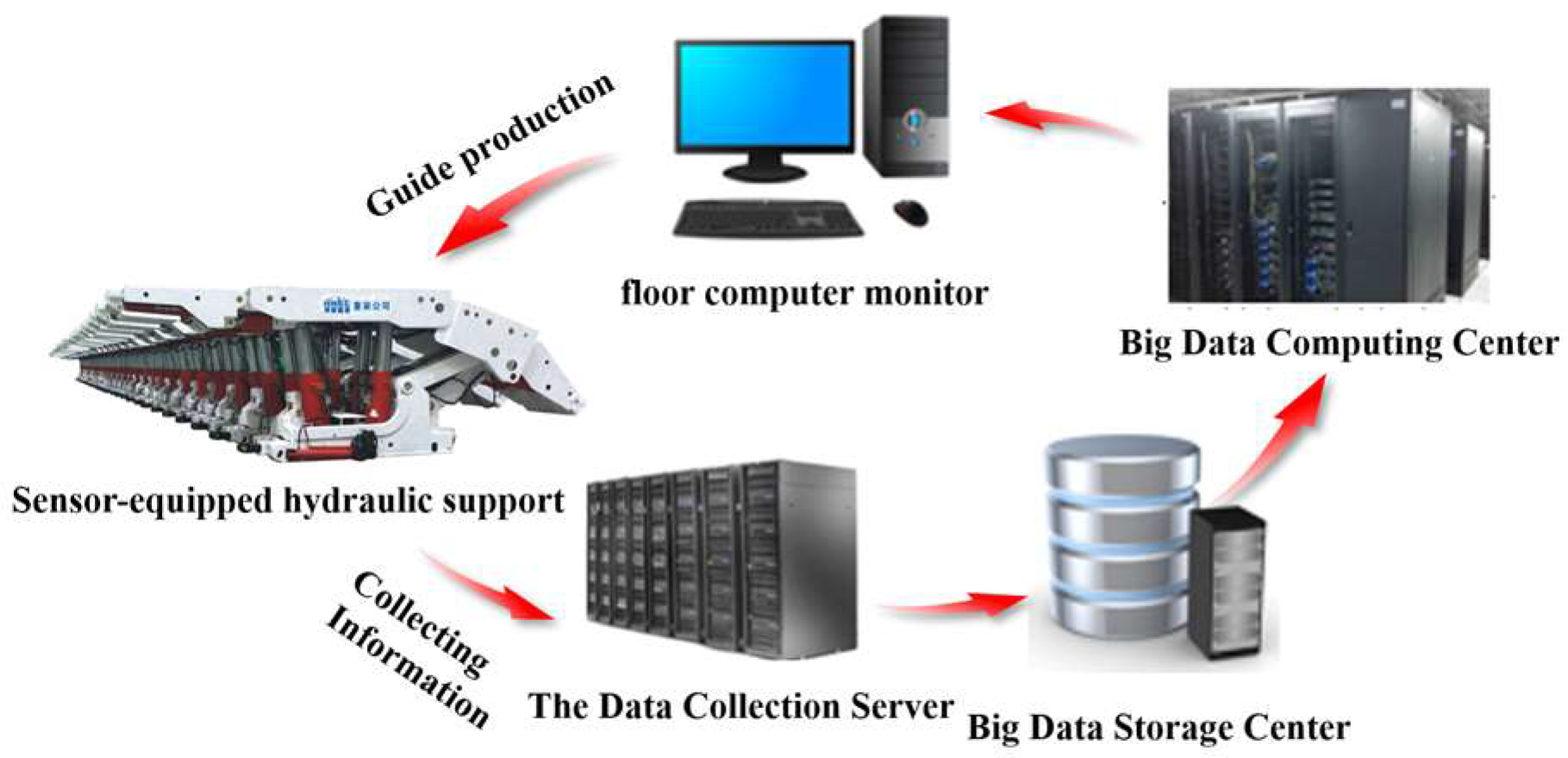
2.2. Monitoring of Support Resistance Data

The support center distance of the Meihuajing coal mine is 1.6 m, the gap is 10 cm, and the caving method is adopted to manage the roof. The working face adopts a KJ197 coal mine dynamic ground pressure monitoring system, as shown in Figure 1. Firstly, the hydraulic support of the working face collects the support working resistance data through YHY60 pressure monitor and transmits it into electro-hydraulic controller, and each support of the working face is equipped with pressure monitor, and the collection time interval is from 3 to 5 s. Then, it connects to the Gigabit industrial network through network switch to transmit the monitoring data to the ground data collection server and big data storage center through communication protocols or relevant procedures. The data received through the transmission will be pre-processed and formatted through the communication protocol or related procedures.

3. IA-PSO-BP Algorithmic Theory

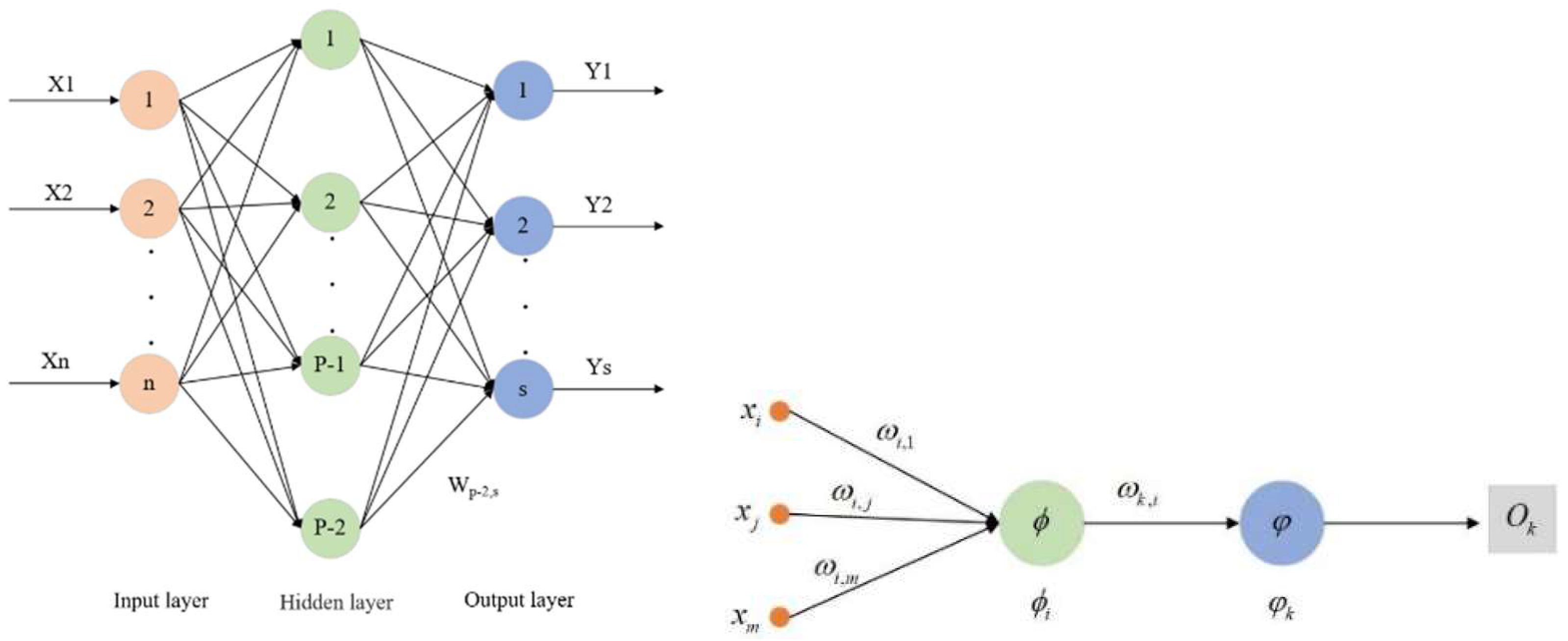
3.1. BP Neural Network

The BP neural network is a multilayer feedforward network that uses the error backpropagation algorithm. This algorithm was proposed by McClelland and other scholars in the mid-1980s. The BP neural network is highly suitable for modelling support resistance due to its simple implementation, small computational requirements, high reliability, and strong nonlinear mapping ability. The network comprises input, hidden, and output layers, with neurons in each layer not connected to each other. However, the neuron points in adjacent layers are connected, as shown in Figure 2.

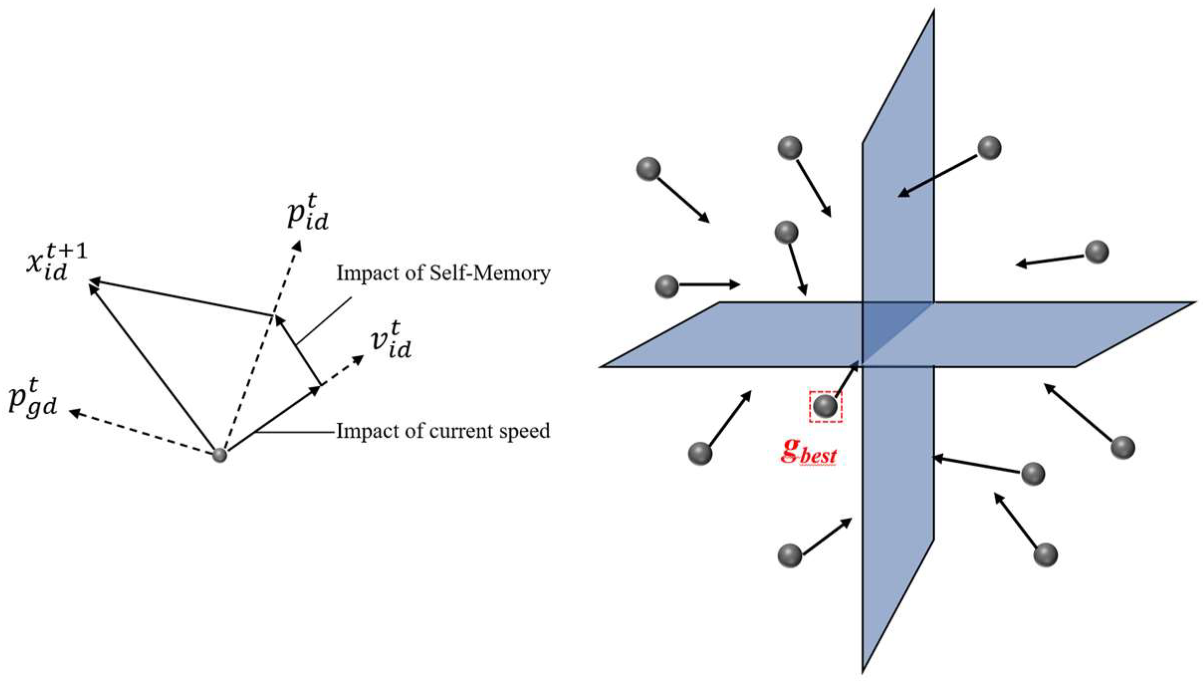
3.2. Particle Swarm Optimization Algorithm (PSO)

Each potential solution of an optimization problem is represented as a particle in the search space. Each particle has a fitness value determined by the optimization function being optimized. Additionally, each particle has a velocity that determines the direction and distance of its next movement. The update of particle positions is illustrated in Figure 3.
In Figure 3, v is the velocity of the particle’s movement; p represents the best position found by the particle. The particle swarm algorithm is initialized with a group of random particles, and then the optimal solution is found through iterations. In each iteration, each particle updates its velocity and position by comparing two extremes. The first extreme is the best solution found by the particle itself, referred to as individual best (pbest); the other extreme is the best solution found by the entire population, referred to as global best (gbest). The remaining particles in the swarm then follow the current best particle to search in the space.
In a D-dimensional space, N particles form a cluster, where the i-th particle is denoted as a D-dimensional vector.
X i = ( x i 1 , x i 2 , , x i D ) , i = 1 , 2 , , N
The velocity of the i-th particle is also a D-dimensional vector.
V i = ( v i 1 , v i 2 , , v i D ) , i = 1 , 2 , , N
The optimal position found by the entire particle swarm up to now is referred to as the global optimum.
g b e s t = ( p g 1 , p g 2 , , p g D )
Once these two optimal values have been found, the particles update their velocity and position according to the following two formulae:
v i , d ( t + 1 ) = ω   ·   v i , d ( t ) + c 1 r 1 [ p i , d x i , d ( t ) ] + c 2 r 2 [ p i , d x i , d ( t ) ]
x i , d ( t + 1 ) = x i , d ( t ) + v i , d ( t + 1 )
In the formula, w is referred to as the inertia factor; c1 and c2 are learning factors, also known as acceleration constants, typically taken from the range from 0 to 4; r1 and r2 are uniformly distributed random numbers within the range from 0 to 1.
Due to its efficient search capability, the particle swarm optimization (PSO) algorithm is advantageous in obtaining optimal solutions in multi-objective contexts. Moreover, the PSO algorithm demonstrates good versatility, making it suitable for handling various types of objective functions and constraints. It can also be easily integrated with traditional optimization methods, thereby improving its own limitations and achieving more efficient problem-solving.

3.3. IA-PSO Algorithm

The particle swarm algorithm uses a random function to initialize a population of particles and uses the adaptation value to evaluate the system when used to perform a random search of the population. In the early stage of searching the solution space of the particle swarm algorithm, the optimal solution can be found very quickly but it is generally a local optimal point, and many times it cannot meet the accuracy requirements [25]. However, if you set a larger value of acceleration factor, maximum speed, etc., the particle swarm algorithm is very likely to fail to obtain the optimal solution, resulting in the inability to converge; if the algorithm converges, then there exists a particle swarm. Each particle will be close to the optimal solution, which inevitably leads to the swarm of particles having a tendency toward homogenization (loss of diversity of particles), so that in the later operation of the algorithm, the convergence speed will become slower, and when the algorithm obtains a certain degree of the optimal solution it cannot continue to optimize, or it will obtain a relatively low accuracy [26]. In order to solve these defects and deficiencies of the particle swarm algorithm, the particle swarm algorithm is improved by using the immunization algorithm, and the algorithm obtained is called the immunization particle swarm algorithm. While overcoming the defects of BP network, the concentration selection mechanism of the immune algorithm is used to maintain the diversity of particles and enhance the global optimization seeking ability of particles. And based on the hydraulic bracket working resistance data, it realizes the early warning prediction of the change rule of the top plate mineral pressure change law of the comprehensive mining face under the coal mine. The flowchart is shown in Figure 4.
The steps of the IA-PSO algorithm are as follows:
Step 1: Initialize c1 and c2 and the number of particle population M;
Step 2: Generate the position xi of M particles(antibodies) and their velocity vi by random mapping by Logistic regression analysis method, where i = 1, 2, …, M, form the initial particle population P0;
Step 3: Generate immune memory particles. Construct the fitness function and calculate whether the fitness value of the particles in the current particle population P satisfies the end condition of the algorithm, if it does, end and output the result, otherwise continue to run;
Step 4: Update the local and global optimal solutions;
Step 5: Then generate N new particles (antibodies) by mapping from logistic regression analysis method;
Step 6: Particle (antibody) selection based on concentration selection mechanism. Calculate the probability of generating N + M new particles (antibodies) using the percentage of similar antibodies in the population;
Step 7: Select N particles (antibodies) in the immune memory particle (antibody) library according to the probability from the largest to the smallest to form the particle (antibody) population P, and then go to the third step.

4. IA-PSO-BP Support Pressure Prediction Algorithm

4.1. Data Source

The dataset is derived from the No. 232205 fully mechanized mining face of the Meihuajing coal mine in Ningxia. It covers the time period from 8:00 on 1 August 2022, to 8:00 on 31 October 2022, and includes a total of 25,920 monitoring data points for the support resistance. The data was sampled every 5 min, and the unit of measurement is MPa. The support pressure monitoring data was preprocessed using the method described in Section 3.2 and then normalized. The dataset contains 25,500 data points. Statistical calculations show that the mean value of hydraulic support resistance after preprocessing is 17.6, with a standard deviation of 12.1. The minimum and maximum values are 0.3 MPa and 43.4 MPa, respectively. To evaluate the prediction performance of the established ground pressure prediction model on different data volumes, the preprocessed dataset is divided into three segments based on time periods. Table 2 shows the information table for the support pressure dataset.

4.2. Data Preprocessing and Normalization

4.2.1. Data Preprocessing

Due to the harsh underground mining environment in coal mines, it is challenging to obtain intact monitoring data. The failures of monitoring equipment and the inherent flaws in sampling algorithms may result in the inclusion of various forms of noise in the data. Therefore, in order to improve the prediction accuracy of the model, it is necessary to first remove outliers, interpolate missing values, and delete duplicate values in the original support pressure monitoring data.
(1)
Outlier value handling
This article adopts the Pauta criterion [27] to calculate the standard deviation of the data and sets the interval based on a certain probability. When the error exceeds this interval, it is considered as an outlier, and the data that reaches the outlier status is regarded as an abnormal data. The formula for determining outliers is shown below, where x is the calculated arithmetic mean and σ is the standard deviation.
σ = i = 1 n ( x i x ) 2 n 1
| x i x | > 3 σ
(2)
Missing value handling
To ascertain the validity of each sensor’s mining pressure data, a calculation formula for the data missing rate is established, as shown in Formula (5).
d e l e t i o n _ r a t e : d r = 1 s 1 s 0
In Formula (5), S0 is the theoretically monitored total data volume of the ground pressure sensor, while S1 is the effective data volume collected by the sensor (including missing values resulting from outlier processing, which are considered invalid data). Assuming a threshold value of 0.2 (indicating at least 80% of valid data presence), if dr is greater than this threshold, the ground pressure monitoring data from this sensor is deemed unusable and can be directly deleted. Conversely, if dr is less than or equal to this threshold, the ground pressure monitoring data from this sensor is considered usable.
(3)
Duplicate values handling
When the underground coal mine will stop mining due to maintenance or mining equipment failure, at this time there is no mining influence, the working face stress basically does not change significantly, which leads to the data monitored by the underground monitoring equipment for a long time to change very little or even not change at all, thus creating a large number of meaningless duplicate values. In order to reduce the amount of data, avoid the model processing a large number of invalid data, and improve the convergence speed and prediction accuracy of the mineral pressure manifestation model, it is necessary to identify and eliminate the duplicate values in the mineral pressure monitoring data. The most common and convenient way to identify duplicate ground pressure values is to sort the ground pressure data first, and the duplicates are necessarily adjacent to each other, and then keep the first data of the duplicate segment and delete all the data after it.

4.2.2. Data Normalization

Due to the large volume and dimensionality of the original ground pressure monitoring data, the time complexity of computer processing is high. Preprocessing can reduce the data dimensionality. Therefore, after handling the outliers, missing values, and duplicate values in the original support pressure monitoring data, normalization is still required. For the support pressure data sequence x i = ( x 1 , x 2 , x N 1 , x N ) , this paper adopts Formulas (6)–(8) to normalize the data sequence, transforming the original ground pressure monitoring data into data within the range from −1 to 1. This eliminates the inconvenience caused by the magnitude of the data sequence for subsequent data analysis and ensures the comparability of the data.
x i = x i μ σ
μ = i = 1 N x i N
σ = i = 1 N ( x i μ ) 2 N 1
In the formula above, xi is the raw data, xi′ is the normalized data, and μ is the mean of the data sequence, σ is the standard deviation of a data series.

4.3. Design of IA-PSO-BP Neural Network Model

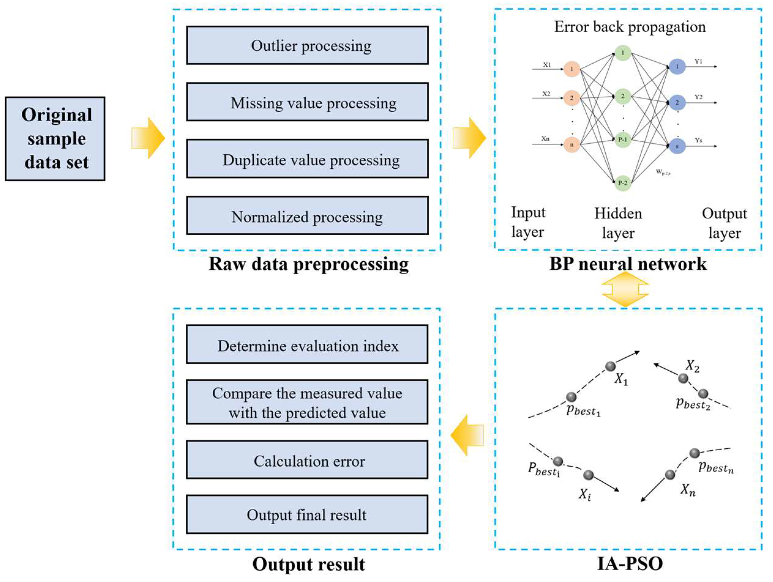
4.3.1. Model Concept

This paper takes the BP network as the regression model, uses the mining pressure data sequence as the model input, and aims to predict the future mining pressure values. However, the BP network often suffers from slow convergence speed and the problem of getting stuck in local optimal states due to the modification of weights and thresholds in the negative gradient direction of the error function. The IA-PSO algorithm optimizes the weights and thresholds of the BP network, overcoming its inherent defects and improving the training speed and prediction accuracy. Additionally, it addresses the problem of slow convergence speed caused by the decrease in particle diversity in the later stage of the PSO algorithm.
Figure 5 shows the process for collecting on-site monitoring data, establishing a training sample dataset, and preprocessing the sample data by handling abnormal values, missing values, duplicate values, and normalization. The preprocessed data sequence is then used as input for the model. The hyperparameters of the BP network are optimized using the immune particle swarm hybrid algorithm. Finally, the predicted values are compared with the actual measured values, and the prediction error is calculated.

4.3.2. Construction of Populations and Fitness Function

To establish the mapping of BP network connection weights and thresholds to PSO particle dimensions using training sample data as particle populations, it is assumed that the number of neurons in the input layer, hidden layer, and output layer of the BP network are I, H, and O, respectively, and the dimensionality of the PSO particles is D = I × H + H × O + O.
The fitness function for the PSO algorithm is calculated using the mean squared error formula output.
F = M S E = 1 n i = 1 n ( y i y i ) 2
In the above formula, yi is the actual output value of the i-th network, and yi′ is the i-the expected value.

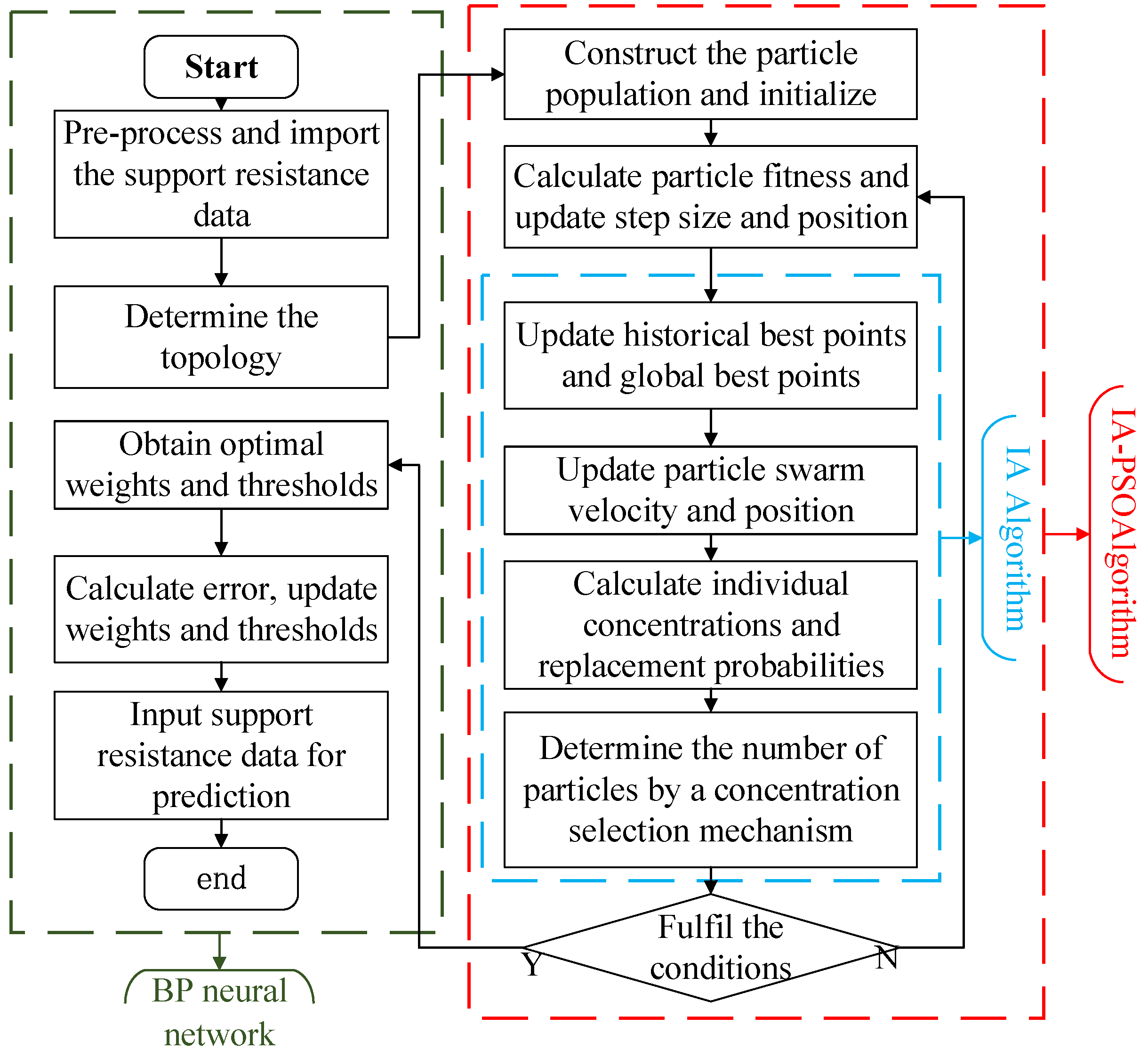
4.3.3. Implementation Steps of the Model

Then IA-PSO is used to optimize the weights and thresholds of BP network, which overcomes the defects of the BP network while maintaining the diversity of the particles using the concentration selection mechanism of the immunized algorithm, and enhances the global optimization-seeking ability of the particles, and the specific steps are as follows:
Input: Mining pressure data sequence: P
Step 1: Initialization
(1)
BP network learning parameter settings: Determine the activation function, training function, learning rate (lr), target error (goal), and maximum iteration count (epochs) based on the training sample data.
(2)
Parameter Settings for IA-PSO Algorithm: The parameters include the number of particles N, the initial positions xi and velocities vi of the particles, the acceleration constants c1 and c2, the inertia weight w, and the individual best value pbest and global best value gbest.
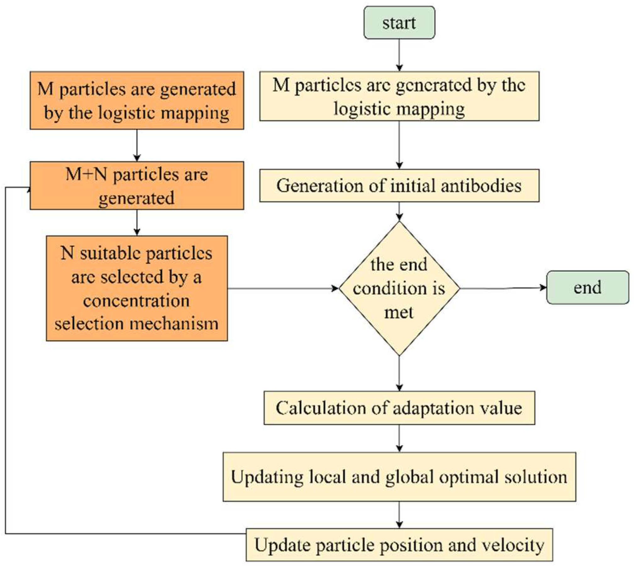
Step 2: Iterative Updates
(1)
Calculate the fitness F(xi) of each particle, and determine the individual best value and global best value.
(2)
Update the position and velocity of the particles, and update the individual and global best values for the particles.
(3)
Calculate the individual concentration and replacement probability, and use a concentration selection mechanism to select N suitable particles.
Step 3: Determine whether the following conditions is satisfied, if so, go to Step 4, otherwise go to Step 2.
(1)
The training error reaches the required accuracy.
(2)
Stops iterating when the maximum number of iterations for training is reached.
Step 4: Output the global optimal value gbest and assign it to the network weights and thresholds. The algorithm ends.
Output: Trained BP neural network.
The algorithmic procedure of the IA-PSO-BP model mentioned is illustrated in Figure 6.

5. Construction of the IA-PSO-BP Ground Pressure Prediction Model

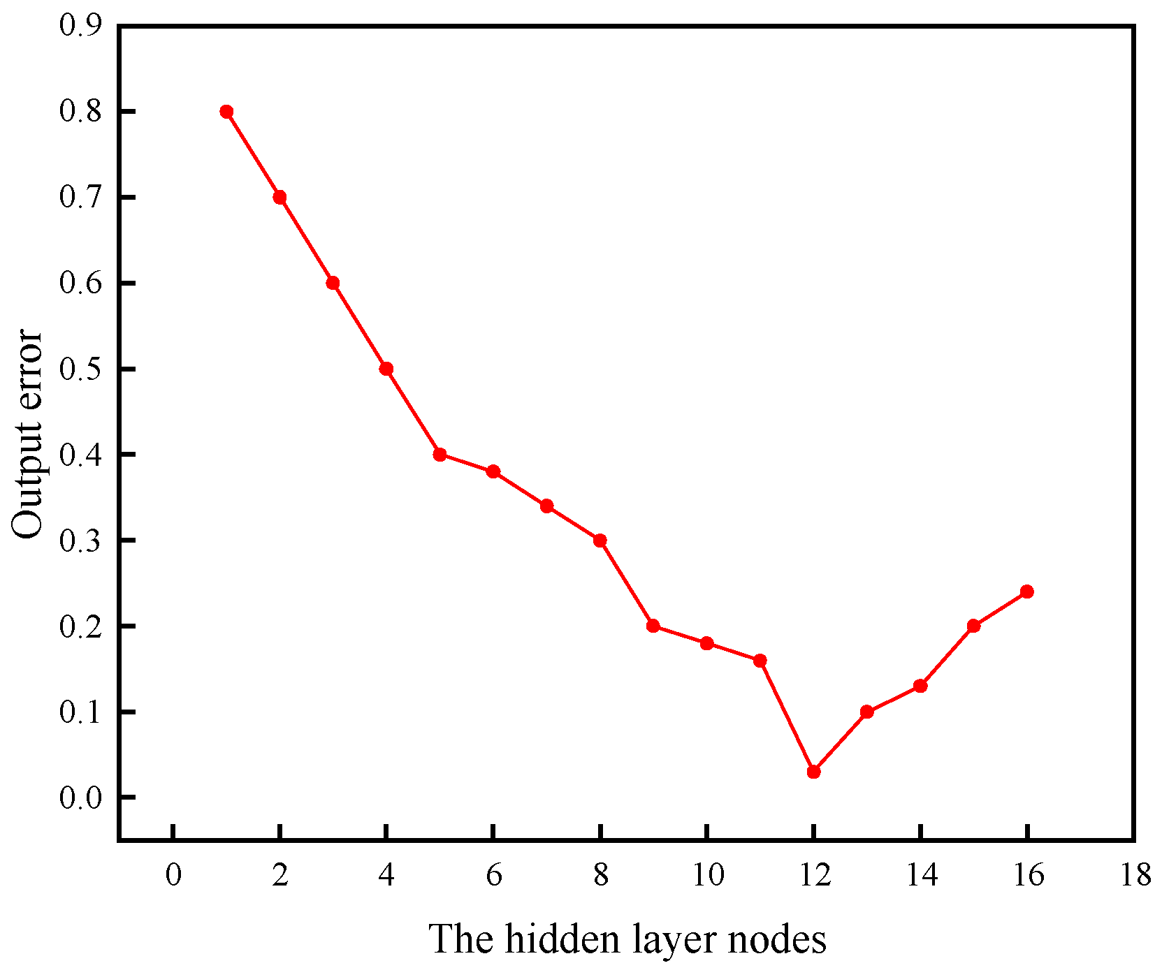
5.1. The Determination of the Topology Structure and Parameter Selection of BP Neural Networks

(1)
Determination of Topological Structure
The determination of the BP network structure mainly includes the determination of the number of layers and nodes in the input layer, hidden layer, and output layer. For the number of layers, the input layer and output layer are fixed at single layer. Since a three-layer BP network with a single hidden layer can achieve nonlinear mapping of any dimension [28], therefore, the topology of single implicit layer is fully capable of fulfilling the requirements of mine pressure data prediction, and the number of nodes in the input and output layers is determined according to the actual problem.
Since the resistance data of the working face support is a continuous time series, there is a certain correlation between adjacent data. If the number of nodes is too small, it will ignore the correlation between data and the trend of data sequences, resulting in low prediction accuracy. On the contrary, if the number of nodes is too large, it will not only improve the prediction accuracy of the model but also increase the complexity of calculations, leading to slow convergence or inability to converge. According to the calculation result lbest = 11 in Section 4.3, the number of nodes in the input layer is set to 11.
This study calculates H ≈ 4 based on the commonly used empirical formula H = I + O + b , the initial value of the number of hidden layer nodes is set to 4. By changing the number of hidden layer nodes through repeated testing, the variation of the hidden layer nodes with the error is obtained as shown in Figure 7. From the figure, it can be observed that when the number of hidden layer nodes is set to 12, the network output error is minimized. Therefore, the number of hidden layer nodes is set to 12. When the number of nodes in the implicit layer exceeds 12, the model is overfitted, in other words, the model complexity is higher than the actual problem, and the overfitting leads to an increase in the generalization error. A reasonable number of hidden nodes can control the complexity of BP neural networks to some extent.
The number of neurons in the output layer depends on the actual requirements. In this model, which aims to predict the working resistance of the roof in mining face, the output variable is the support resistance. Therefore, the number of nodes in the output layer is set to 1.
(2)
Parameter Selection for BP Neural Network
The selection of parameters for the BP network primarily involves choosing the activation function, training function, target error goal, maximum number of iterations (epochs), and learning rate (lr). The selection of activation and training functions is based on the distribution characteristics of the training dataset. The target error and maximum number of iterations are determined based on the specific problem requirements, while the learning rate is dynamically selected according to the change in network prediction error. In this paper, the goal is set to 0.001, epochs to 2000, and lr to 0.05, in accordance with the actual requirements. The training dataset is normalized using the Z-Score method, resulting in a dataset that follows a standard normal distribution. The ReLu function is commonly selected as the activation function for the hidden layer due to its constant gradient, which can accelerate the convergence speed of the BP network. The Pureline function, a linear activation function, is chosen for the output layer to increase the range of output values. The network training function selected is the widely used Trainlm function.

5.2. Parameter Setting for IA-PSO Optimization Algorithm

(1)
Population size N
The population size N affects the computational complexity and search capability of the algorithm. The PSO algorithm does not require a high population size and generally achieves good solution performance when the value is set between 20 and 40. For more difficult or specific types of problems, 100 to 150 particles may be needed. A larger population size expands the search space, making it easier to find the global optimum solution. However, it also increases the running time. In order to balance the running time and optimization performance of the algorithm, this study sets the population size to 100.
(2)
Inertial weight w.
This study employs a dynamic inertia factor to enable the algorithm to search a larger solution space at the beginning of optimization to find suitable particles. Then, it gradually narrows down to a smaller region for a more refined search to accelerate convergence speed. The initial value of w, wstart, is set to 0.9, and it linearly decreases with each iteration until it reaches the minimum value of wend = 0.4. This is performed to achieve the optimization objectives.
The calculation formula for the linearly decreasing inertia weight with the number of iterations is as follows.
w d = w s t a r t ( w s t a r t w e n d ) × d K
In the formula, wd represents the inertia weight at the d-th iteration, where d is the current iteration number, K is the total number of iterations, and wstart = 0.9 and wend = 0.4.
(3)
Particle acceleration constants c1 and c2
The weights c1 and c2 affect the acceleration of particles towards their personal best (pbest) and the global best (gbest). Typically, c1 and c2 are set such that c1 + c2 ≤ 4, with many cases using c1 = c2 = 2 which indicates equal importance given to both directions. However, setting the learning factors as constants can hinder the maintenance of particle swarm diversity, leading to premature convergence and trapping in local optima. To address this issue, this paper proposes an adaptive learning factor.
The formula for calculating the adaptive learning factor is as follows.
c 1 d = c 1 max d ( c 1 max c 1 min ) K
c 2 d = c 2 min + d ( c 2 max c 2 min ) K
In the formula, d is the current iteration number, K is the total number of iterations, c 1 d is the learning factors at the d-th iteration, c1max and c2min are the maximum learning factors with values of c1max = c2max = 2.2, and c1min and c2min are the minimum learning factors with values of c1min = c2min = 0.2.
In summary, the main parameter settings of the IA-PSO algorithm in this paper are presented in Table 3.

5.3. Determination of Optimal Length for Historical Data

Using dataset 1 as the training sample set for the model, in the same experimental environment, with a fixed prediction data length. by continuously changing the historical data length l, selecting the mean squared error (MSE) as the loss function, first determine the optimal search range for the historical data length, and then determine the optimal historical data length lbest within the search range.
Figure 8 shows that the model prediction error fluctuates when the length l is between 50 and 1000. The error increases as the length of historical data increases. When the length of historical data is between 50 and 100, the model prediction error increases gradually. When the length l is between 50 and 100, the model prediction error increases gradually. Therefore, it is recommended to search for the optimal length of the historical data within the range of 1 to 60.
The MSE exhibits a fluctuating trend within the optimal historical search range of 1 to 60. Overall, the error increases as the length l increases. The error is minimized when length l is 11, thus, determining the optimal length of historical data as lbest = 11.

6. Results and Analysis

6.1. Model Evaluation Metrics

To evaluate the predictive performance of the ground pressure prediction model based on IA-PSO-BP, this study adopts three indicators: mean absolute error (MAE), mean square error (MSE), and correlation coefficient (R2) to evaluate the predictive performance of each model on the test set. The closer the MAE and MSE are to 0, and the closer the correlation coefficient is to 1, the better the fitting performance, and the higher the prediction accuracy of the model. The formulas for calculating MAE, MSE, and R2 are as follows:
M A E = 1 N i = 1 N | y i y i |
M S E = 1 N i = 1 N ( y i y i ) 2
R 2 = 1 i = 1 N ( y i y i ) 2 i = 1 N ( y i y i ) 2
N is the number of samples in the test set, yi is the measured value of mining pressure, y i is the predicted value of mining pressure, and y i ¯ is the mean value of the test set samples. Here, i = 1, 2, 3, ..., N.

6.2. Model Convergence Speed and Loss Value

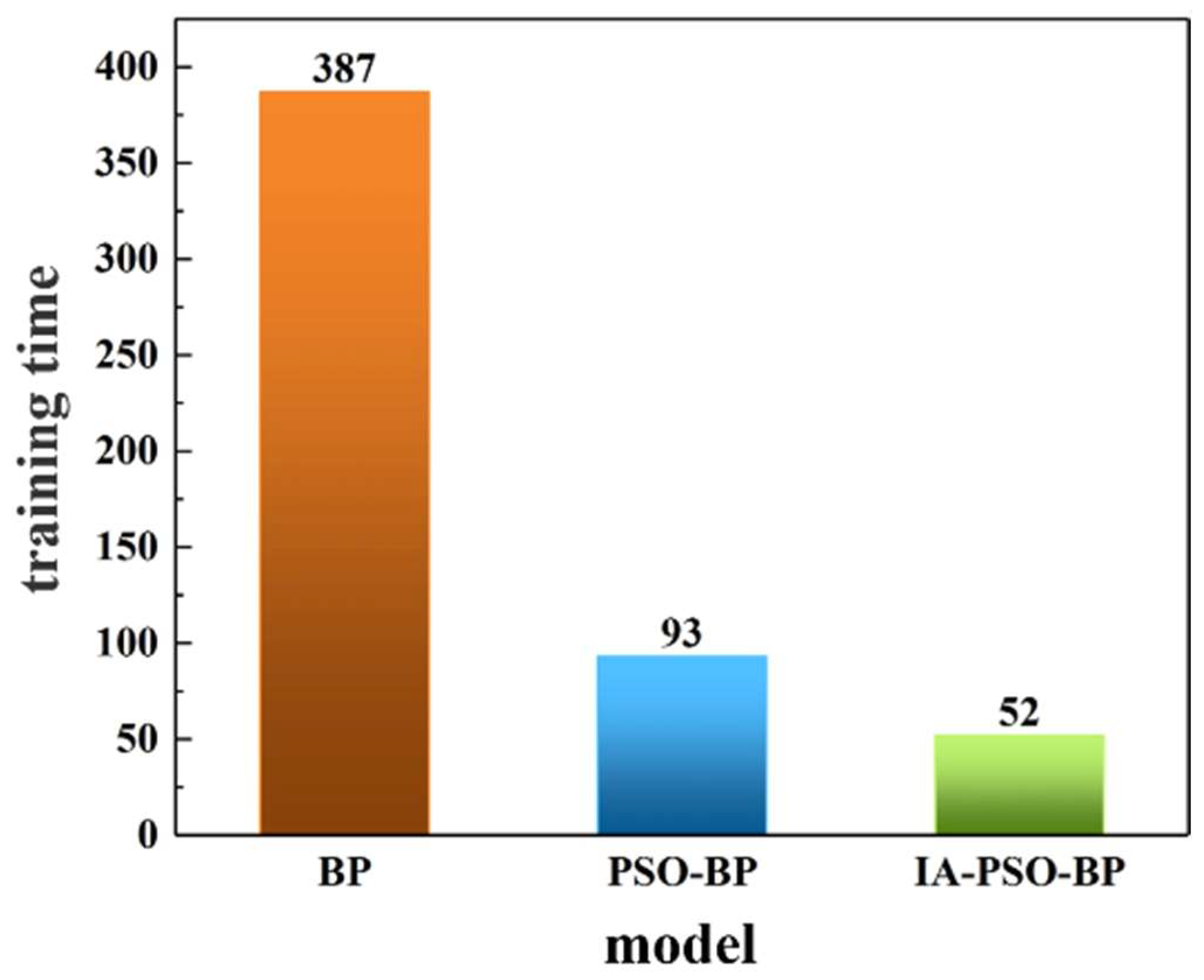
6.2.1. Convergence Speed
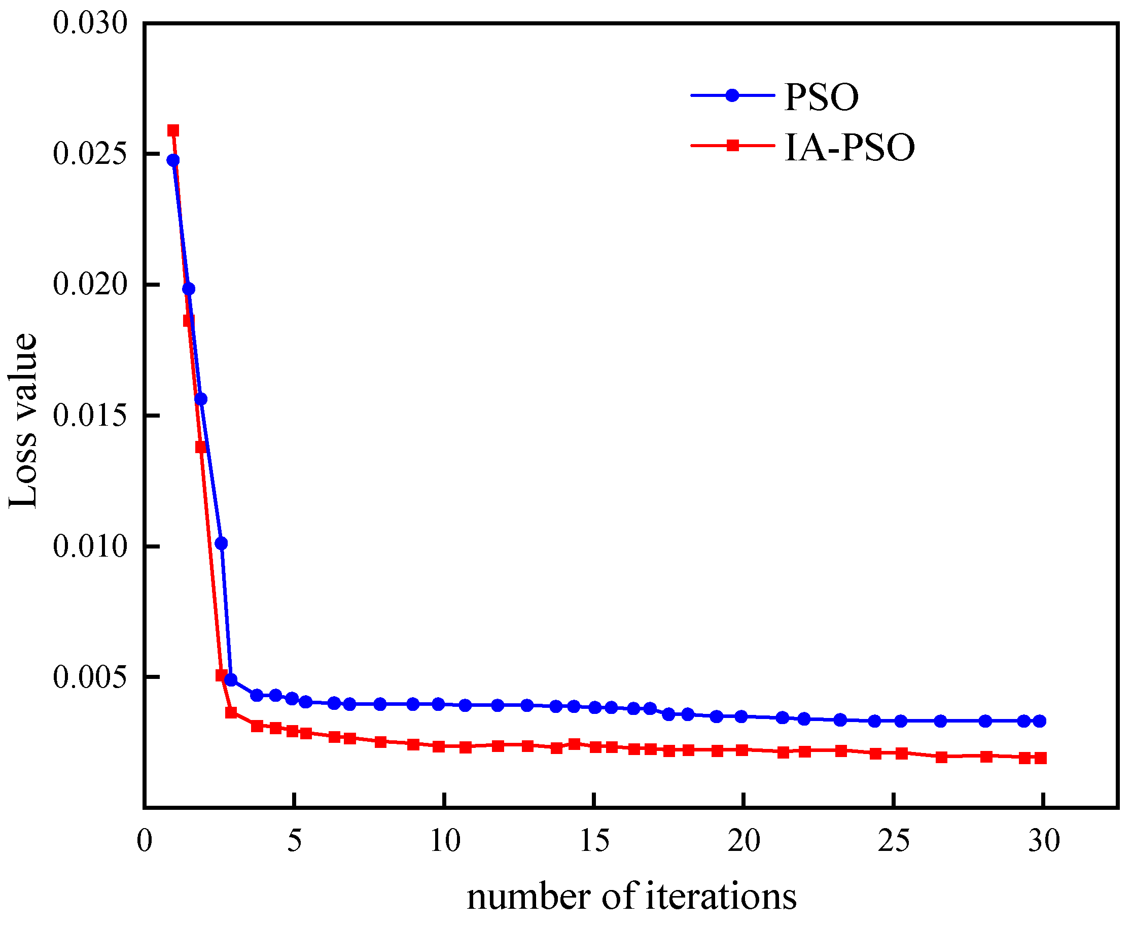
After preprocessing and normalization of the data, the BP model, PSO-BP model, and IA-PSO-BP model were used for training. The training times for each model that met the target error were shown in Figure 9.
Figure 9 showed that the prediction model met the accuracy requirements after 52 iterations, while the BP and PSO-BP prediction model required 387 and 93 iterations, respectively. The results demonstrated that the IA-PSO-BP prediction model trained approximately eight times faster than the BP prediction model while meeting the same accuracy requirements. Additionally, the PSO-BP prediction model trained about two times faster. These findings suggested that the IA-PSO algorithm could effectively address the issue of slow convergence speed in the BP network, resulting in a significant improvement in training speed.

6.2.2. Loss Value

PSO and IA-PSO were utilized to optimize the hyperparameters of the BP model, respectively. The same number of iterations were set for each epoch, and MSE was chosen as the loss function to calculate the loss values of the model optimized by different algorithms. Figure 10 illustrates the comparison of loss values for each optimization algorithm.
Figure 10 shows that the loss value of both PSO and IA-PSO optimization algorithms gradually decreased with increasing iterations. The rate of decline slows down and tends to stabilize with more iterations, indicating that both algorithms can optimize the hyperparameters of model. However, the IA-PSO optimization algorithm achieves the fastest decrease in loss overall. The PSO optimization algorithm is known for its stability after a certain number of iterations and its lower loss value compared to other optimization algorithms. However, in the middle and later stages of iteration, the algorithm tends to homogenize particles, resulting in a decrease in particle diversity and an increased risk of falling into local optimization. On the contrary, the concentration selection mechanism of the immune algorithm enhances the diversity of particles, resulting in the IA-PSO optimization algorithm being able to gradually reduce the loss value in the later stages.

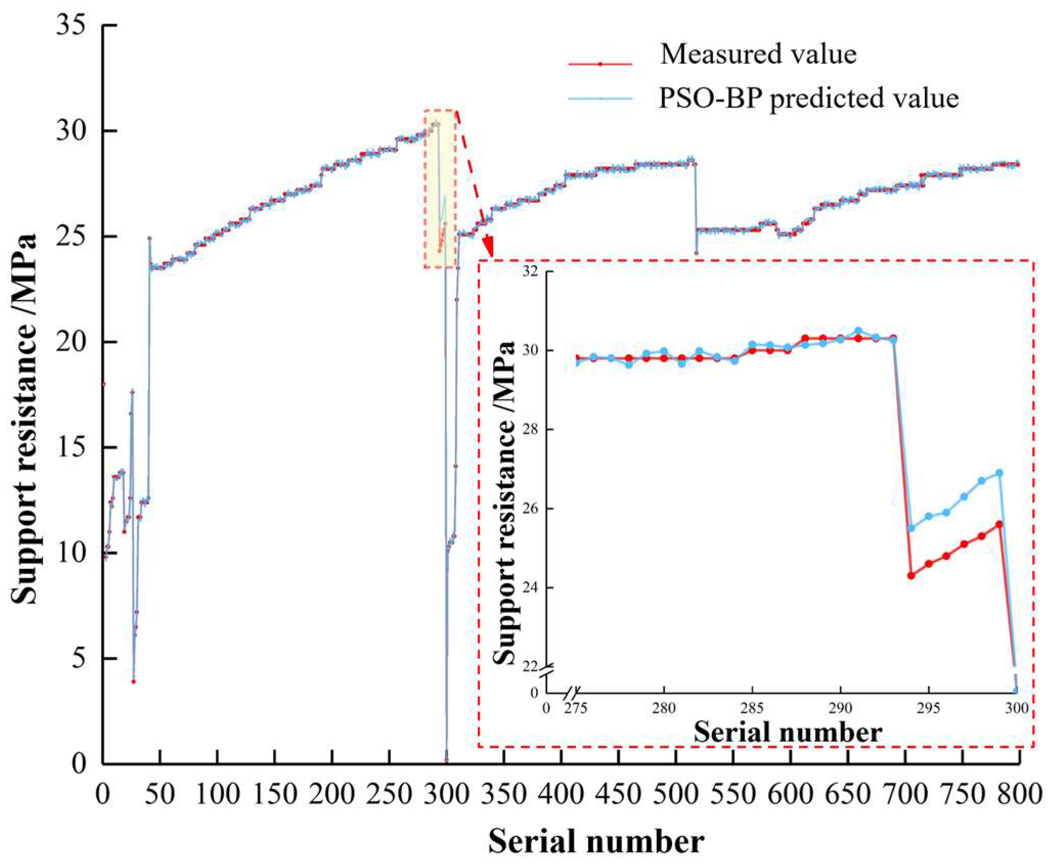
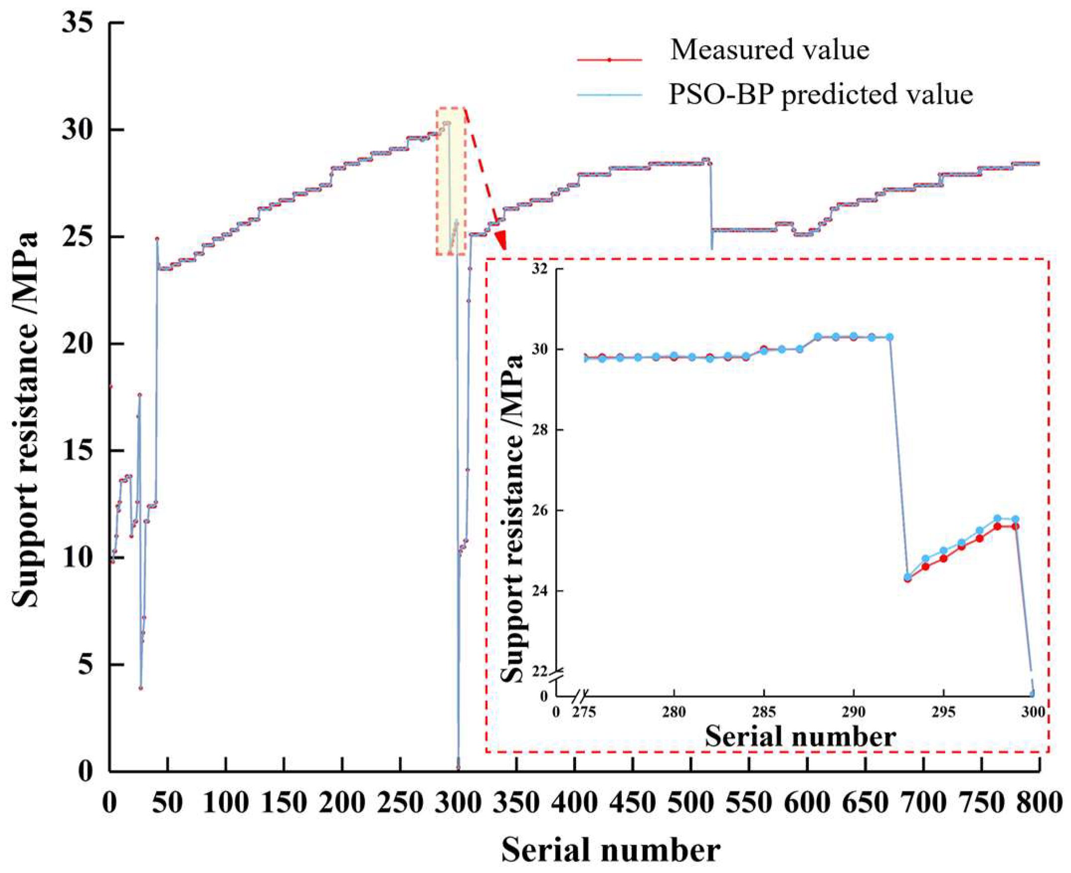
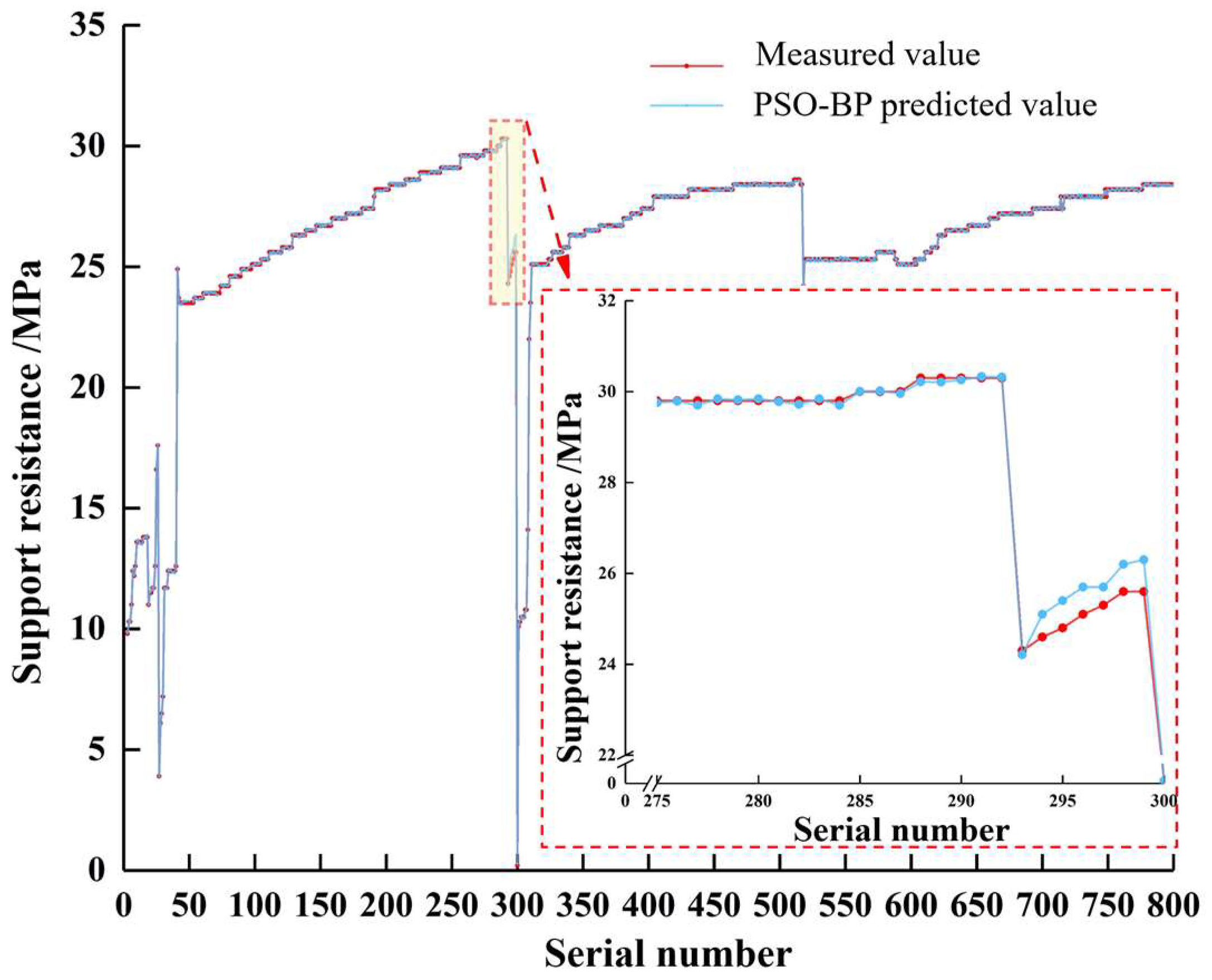
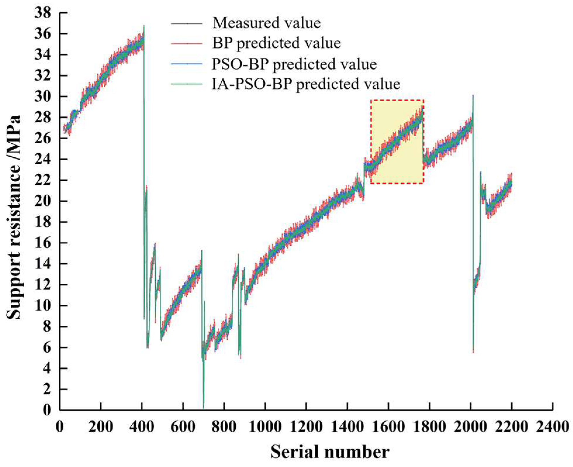
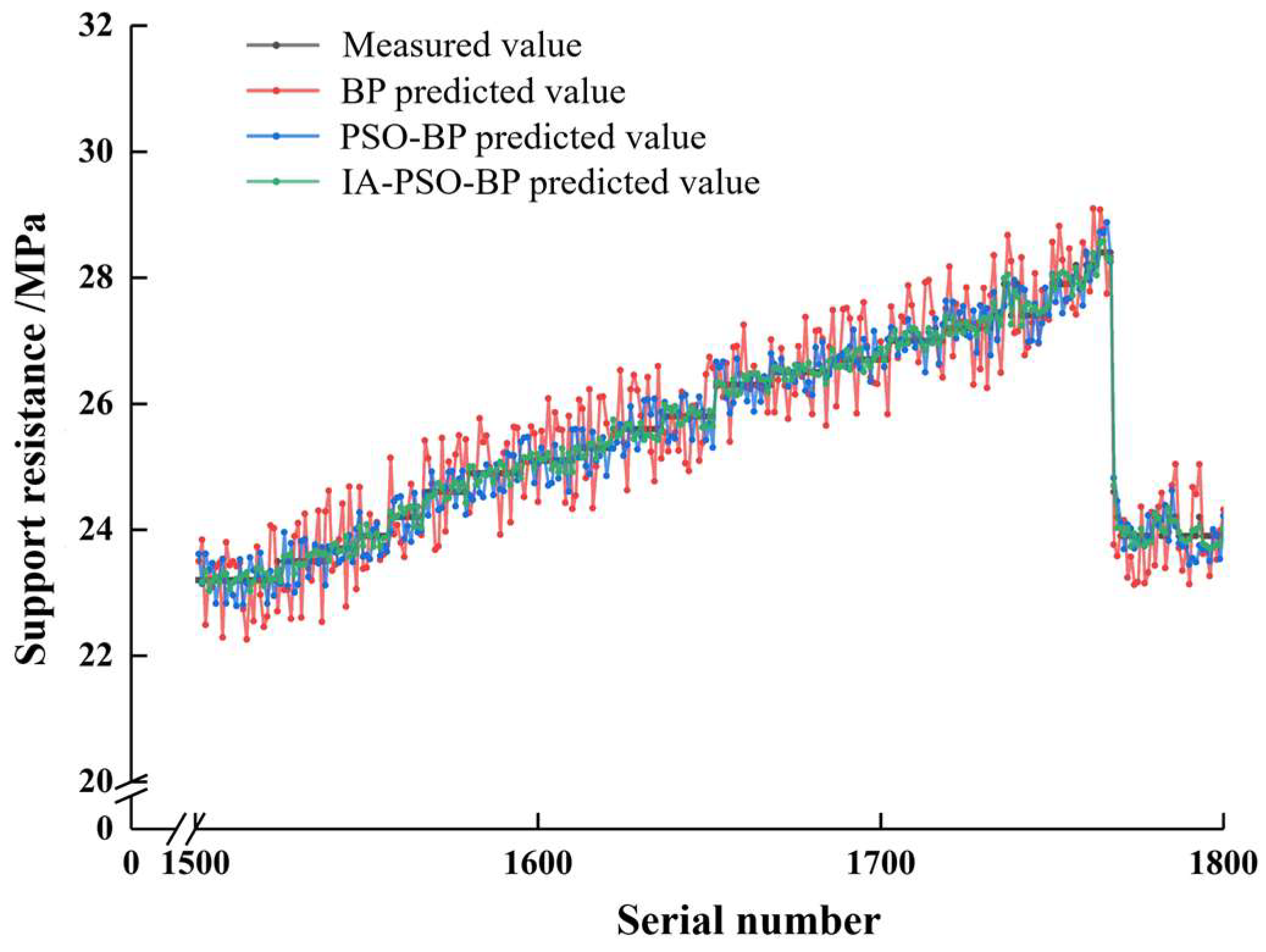
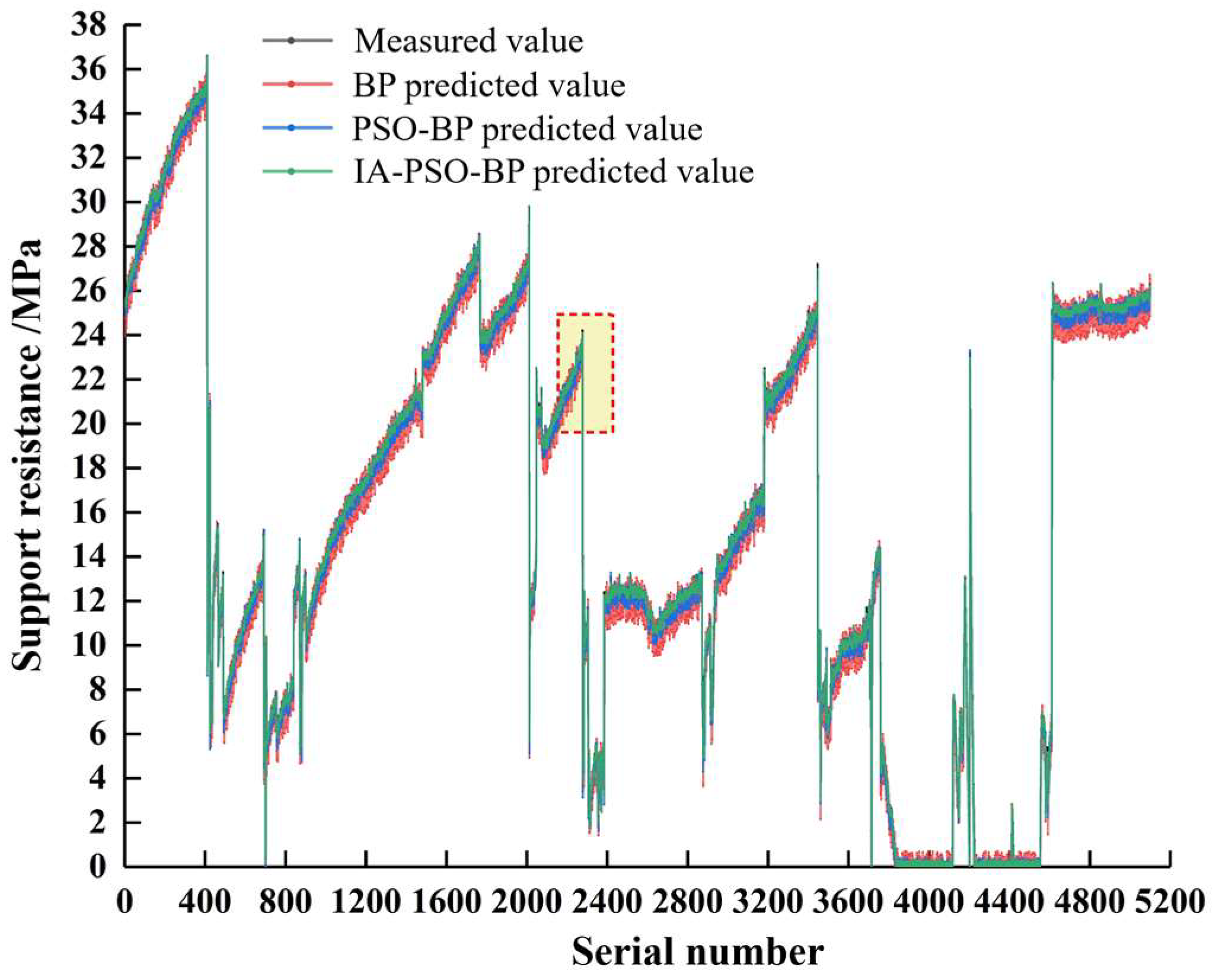
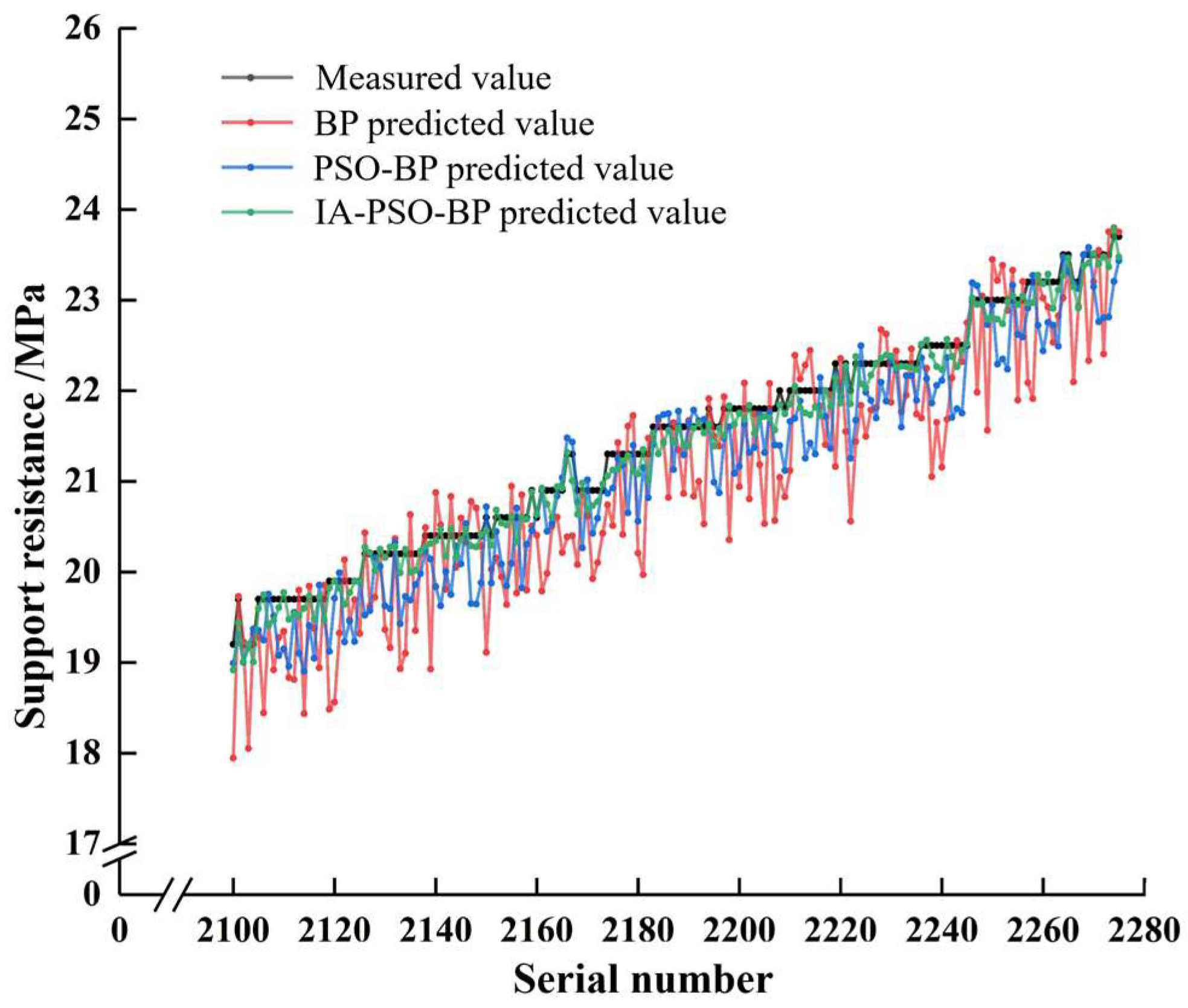
6.3. Comparison of Ground Pressure Prediction Performance among Different Models

The first 80% of each dataset is allocated as the training set for each predictive model, while the remaining 20% is used as the test set. The division of each dataset is presented in Table 4.
First, the prediction results of various models are tested on dataset 1. The fitting effects of the BP, PSO-BP, and IA-PSO-BP prediction models on the actual values of the test set are compared, as shown in Figure 11, Figure 12 and Figure 13.
Among them, the bottom right corner of Figure 12 to Figure 13 is a partial magnification of the red-marked area in the figure. It can be seen that the fitting effect of the predicted values and measured values of the PSO-BP and IA-PSO-BP models is good, conforming to the periodic variation pattern of the data. However, there is a significant difference between the predicted values and measured values of the BP model. The predicted values of the BP model optimized by IA-PSO are closest to the measured values.
The MAE, MSE, and R2 of the predicted values and measured values of each model are calculated, and the results are shown in Table 5.
From Table 5, it can be seen that on dataset 1, the IA-PSO-BP model reduces the MAE of the BP model by 22.21%, reduces the MSE by 28.35%, and increases the R2 by 23.03%; compared to the PSO-BP model, the IA-PSO-BP model reduces the MAE by 12.73%, reduces the MSE by 17.86%, and increases the R2 by 7.7%. Therefore, the IA-PSO-BP model demonstrates significantly better predictive performance than the BP model and the PSO-BP model. The IA-PSO optimized BP model reduces the error compared to the PSO optimized BP model, indicating that the IA-PSO algorithm overcomes the problem of the BP network easily falling into local optima and the decrease in optimization ability caused by the decrease in particle diversity in the later stage of PSO. Therefore, using the IA-PSO-BP model to predict the support resistance data on dataset 1 is feasible.
Then, the predictive performance of various models on dataset 2 is tested, and the fitting effect of the BP, PSO-BP, and IA-PSO-BP predictive models on the test set actual values is compared, as shown in Figure 14. A local magnification of the red area in the figure is shown in Figure 15. From Figure 14, it can be seen that the predictive values of all models fit well with the actual values, and they conform to the periodic variation pattern of the data. According to Figure 15, the IA-PSO-BP predictive model exhibits exceptional predictive performance and accuracy, as evidenced by its close approximation to actual values.
We calculated the MAE, MSE, and R2 for the predicted values of each model compared to the observed values. The calculation results are shown in the following table.
From Table 6, it can be seen that on dataset 2, the IA-PSO-BP model reduces the MAE of the BP model by 22.98%, reduces the MSE by 33.52%, and increases the R2 by 20.1%; compared to the PSO-BP model, the IA-PSO-BP model reduces the MAE by 12.43%, reduces the MSE by 20.92%, and increases the R2 by 6.59%. Therefore, the IA-PSO-BP model has the closest prediction to the actual values and the smallest error. This indicates that using the IA-PSO-BP model on dataset 2 has a good predictive effect.
Based on the data in Table 6 for dataset 2, it was evident that the IA-PSO-BP model outperformed the BP model by reducing the MAE by 22.98%, the MSE by 33.52%, and increasing the R2 by 20.1%. In comparison with the PSO-BP model, the IA-PSO-BP model reduces the MAE by 12.43%, the MSE by 20.92%, and increases the R2 by 6.59%. Therefore, the IA-PSO-BP model offers the most accurate results and the smallest error, indicating its efficacy in predicting actual values for dataset 2.
Finally, the predictive results of each model are evaluated using dataset 3. The performance of the BP, PSO-BP, and IA-PSO-BP prediction models on the actual values of the test set is presented in Figure 16. Additionally, Figure 17 provides a zoomed-in view of the red area in the figure. Based on the analysis presented in Figure 16, it can be observed that the accuracy of the predicted values of each model improves as the data volume of the dataset gradually increases, and progressively matches the periodic variation pattern of the data. Furthermore, as illustrated in Figure 17, the predicted values of the IA-PSO-BP prediction model consistently aligns with the actual values, suggesting that this model excels in predictive performance compared to other models.
Calculate the mean absolute error (MAE), mean squared error (MSE), and coefficient of determination (R2) for the predicted values of each model compared to the observed values. The calculation results are shown in the following table.
As shows in Table 7, on dataset 3, the IA-PSO-BP model reduces the MAE by 25.84% and MSE by 12.8% compared to the BP model. It also increases R2 by 18.88%. Compared to the PSO-BP model, the IA-PSO-BP model reduced the MAE by 16.4%, MSE by 6.84%, and increased R2 by 6.3%. Therefore, the IA-PSO-BP model has the smallest prediction error and the best fitting effect. This indicates that the IA-PSO-BP model has the best prediction effect on dataset 3.
In summary, on all three datasets, the IA-PSO optimization algorithm improves the prediction accuracy. It shows lower prediction errors compared to the traditional BP model and PSO-BP model, and higher correlation between predicted values and actual values. The prediction performance is significantly improved, making the IA-PSO-BP prediction model significantly better than other models in rock pressure prediction. Additionally, as shows in Table 5, Table 6 and Table 7, it is evident that the size of the dataset is negatively correlated with the prediction errors of the models, meaning that the larger the dataset, the smaller the prediction errors for each model.

7. Discussion

(1)
Due to the complexity of the underground environment, the monitoring equipment is restricted by the disturbance of the mining project and the installation technology, which leads to the lack of integrity of the monitoring data and the existence of a large number of outliers and missing values, which has a greater impact on the prediction of the actual mine pressure data in the underground.
(2)
The limited nature of the data set affects the prediction accuracy of the model.
(3)
In the future, correlation analysis or data fusion will be performed on different types of monitoring data from the same working face to establish a training data set with a larger data volume and more data types, so as to further improve the accuracy of predicting mine pressure at the working face.
(4)
In the paper, the mine pressure monitoring data of the No. 232205 working face of the Meihuajing coal mine is selected as the data source, and in the future, we need to consider the generalization function of the model, and use the transfer-learning method to use the trained model to predict the mine pressure accurately in the working face under similar geological and mining conditions.
(5)
Establishing a dynamic mine pressure monitoring and early warning and forecasting system for coal mines based on Python, CSS, html and JavaScript programming languages to achieve dynamic visualization monitoring of mine pressure at the working face and intelligent prediction and warning of mine pressure disasters.

8. Conclusions

(1)
By combining the immune algorithm and PSO algorithm, the inherent defects of BP network were surmounted. Furthermore, the problem of slow convergence speed caused by the decrease of particle diversity in the later stage of PSO algorithm was surmounted. A prediction method of working face ground pressure based on IA-PSO-BP was proposed. According to the relationship between the mean square error of network prediction and the length of historical data, the optimal historical support pressure data length lbest = 11 of the ground pressure prediction model was determined.
(2)
The convergence speed of the IA-PSO-BP model was approximately eight times faster than the BP model and two times faster than the PSO-BP model. Meanwhile, the IA-PSO optimization algorithm had the fastest decreasing loss value, which tended to stabilize after a certain number of iterations and was lower than the other optimization algorithms.
(3)
The IA-PSO-BP model achieved the best prediction performance on three different datasets with varying data sizes. As the data size increases, the prediction errors of all models gradually decreased. The IA-PSO-BP model exhibited the smallest MAE and MSE, as well as the largest R2, compared to the BP and PSO-BP models on the three test sets. The average MAE, MSE, and R2 on the three test sets were 0.0751, 0.0123, and 0.9747. Therefore, the IA-PSO hybrid optimization algorithm significantly improved the prediction accuracy of the model.

Author Contributions

Conceptualization, X.L. (Xingping Lai); Methodology, X.L. (Xingping Lai); Software, Y.T.; Validation, Y.T., B.Y. and X.L. (Xiaoming Liu); Formal analysis, L.W. and X.L. (Xiaoming Liu); Resources, L.W. and X.L. (Xiaoming Liu); Writing—original draft, Y.T.; Writing—review & editing, Y.T.; Supervision, X.L. (Xingping Lai) and B.Y.; Funding acquisition, X.L. (Xingping Lai). All authors have read and agreed to the published version of the manuscript.

Funding

This research was funded by Shaanxi Provincial Natural Science Basic Research Project Enterprise Joint Fund, grant number 2019JLZ-04.

Data Availability Statement

Data are contained within the article.

Conflicts of Interest

Author Xiaoming Liu was employed by the company CHN Energy Ningxia Coal Industry Co., Ltd. The remaining authors declare that the research was conducted in the absence of any commercial or financial relationships that could be construed as a potential conflict of interest.

References

  1. Xie, H.; Liu, H.; Wu, G. Quantitative analysis of coal contribution to national Economic Development. China Energy 2012, 34, 5–9. [Google Scholar]
  2. Guo, P.; Wang, T.; Li, D.; Zhou, X. How energy technology innovation affects transition of coal resource-based economy in China. Energy Policy 2016, 92, 1–6. [Google Scholar] [CrossRef]
  3. Qi, Q.; Pan, Y.; Shu, L.; Li, H.; Jiang, D.; Zhao, S.; Zou, Y.; Pan, J.; Wang, K.; Li, H. Theory and technical framework of prevention and control with different sources in multi-scales for coal and rock dynamic disasters in deep mining of coal mines. J. China Coal Soc. 2018, 43, 1801–1810. [Google Scholar]
  4. Wang, J.C.; Xu, J.L.; Yang, S.L.; Wang, Z.H. Development of strata movement and its control in underground mining: In memory of 40 years of Voussoir Beam Theory proposed by Academician Minggao Qian. Coal Sci. Technol. 2023, 51, 80–94. [Google Scholar]
  5. Huang, Q. Mineral pressure characteristics and definition of shallow buried coal seam. J. Rock Mech. Eng. 2002, 21, 1174–1177. [Google Scholar]
  6. Yan, B.; Jia, H.; Yang, Z.; Yilmaz, E.; Liu, H. Goaf instability in an open pit iron mine triggered by dynamics disturbance: A large-scale similar simulation. Int. J. Min. Reclam. Environ. 2023, 37, 606–629. [Google Scholar] [CrossRef]
  7. Ma, Y.; Sun, B.; Li, D. Mine Development Design Expert System Based on Neural Network. In Proceedings of the 24th APCOM Symposium, Montreal, QC, Canada, 31 October–3 November 1993; pp. 161–169. [Google Scholar]
  8. Fei, G. Analysis of the types of coal mine accidents in China from 2006 to 2015. Inn. Mong. Coal Econ. 2017, 22, 120–121. [Google Scholar]
  9. Skrzypkowski, K.; Korzeniowski, W.; Duc, T.N. Choice of powered roof support FAZOS-15/31-POz for Vang Danh hard coal mine. J. Pol. Miner. Eng. Soc. 2020, 21, 175–182. [Google Scholar] [CrossRef]
  10. Jia, B.; Xian, C.; Jia, W.; Su, J. Improved Petrophysical Property Evaluation of Shaly Sand Reservoirs Using Modified Grey Wolf Intelligence Algorithm. Comput. Geosci. 2023, 27, 537–549. [Google Scholar] [CrossRef]
  11. Jia, B.; Xian, C. Permeability measurement of the fracture-matrix system with 3D embedded discrete fracture model. Pet. Sci. 2022, 19, 1757–1765. [Google Scholar] [CrossRef]
  12. Zhou, D.; Zuo, X. Surface subsidence monitoring and prediction in mining area based on SBAS-InSAR and PSO-BP neural network algorithm. J. Yunnan Univ. Nat. Sci. Ed. 2021, 43, 895–905. [Google Scholar]
  13. Qu, S.; Li, P. Research on prediction technology of roof mining pressure based on big data of support resistance. Min. Saf. Environ. Prot. 2019, 46, 92–97. [Google Scholar]
  14. Conover, D.P.; Barczak, T.M. The Niosh shield hydraulics inspection and evaluation of leg data (shield) computer program. In Proceedings of the 21st International Conference on Ground Control in Mining, Morgantown, WV, USA, 6–8 August 2002; pp. 27–38. [Google Scholar]
  15. Wang, J.; Gao, R.; Yu, G.; Gong, W.; Zhu, D. Experimental study on infrared radiation characteristics of overburden movement of self-forming roadway under pressure relief. J. China Coal Soc. 2020, 45, 119–127. [Google Scholar]
  16. Pan, J.F.; Kang, H.P.; Yan, Y.D.; Ma, X.H.; Ma, W.T.; Lu, C.; Lv, D.Z.; Xu, G.; Feng, M.H.; Xia, Y.X.; et al. The method, mechanism and application of preventing rock burst by artificial liberation layer of roof. J. China Coal Soc. 2023, 48, 636–648. [Google Scholar]
  17. Ghosh, G.-K.; Sivakumar, C. Application of underground microseismic monitoring for ground failure and secure longwall coal mining operation: A case study in an Indian mine. J. Appl. Geophys. 2018, 150, 21–39. [Google Scholar] [CrossRef]
  18. Sivakumar, C.; Srinivasan, C.; Gupta, R.N. Microseismic monitoring to study strata behavior and to predict roof falls on a Longwall face at Rajendra Colliery in India. In Proceedings of the 6th Symposium on Rock Burst and Seismicity in Mines (RASIM 6), Perth, WA, Australia, 9–11 March 2005; pp. 135–144. [Google Scholar]
  19. Pan, Y.; Zhao, Y.; Guan, F.; Li, G.; Ma, Z. Study on rockburst monitoring and orientation system and its application. Chin. J. Rock Mech. Eng. 2017, 26, 1002–1011. [Google Scholar]
  20. Wang, E.Y.; He, X.; Li, Z.H.; Zhao, E. Electromagnetic Radiation Technology of Coal Rock and Its Application; Beijing Science Press: Beijing, China, 2009. [Google Scholar]
  21. Li, A.N.; Ling, L.M.; Wang, Z.Y.; Cao, J.R.; Wang, S.W.; Shan, C.H. Numerical simulation of rock burst of horizontal sectional mining of near-vertical coal seam under dynamic load. Coal Eng. 2018, 50, 83–87. [Google Scholar]
  22. He, C.; Hua, X.; Yang, K. Forecast of periodic weighting in working face based on back propagation neural network. J. Anhui Univ. Sci. Technol. (Nat. Sci.) 2012, 32, 59–63. [Google Scholar]
  23. Wu, X.; Lai, X.; Guo, J.; Cui, F.; Wang, Z.; Xu, H. PSO-SVM prediction model of coal pillar width in fully mechanized mining face. J. Xi’an Univ. Sci. Technol. 2020, 40, 64–70. [Google Scholar]
  24. Zhao, Y.X.; Yang, Z.L.; Ma, B.J.; Song, H.H.; Yang, D.H. Deep learning prediction and model generalization of ground pressure for deep longwall face with large mining height. J. China Coal Soc. 2020, 45, 54–65. [Google Scholar]
  25. Huang, M.; Zhang, T.; Wang, J.; Zhu, L. A new air quality forecasting model using data mining and artificial neural network. In Proceedings of the 2015 6th IEEE International Conference on Software Engineering and Service Science (ICSESS), Beijing, China, 23–25 September 2015; pp. 259–262. [Google Scholar]
  26. Lang, J.; He, Q.; Fan, X.; Huang, P.; Zhang, X. Prediction of airflow classification effect of wet coal based on BP neural network. J. China Coal Soc. 2021, 46, 1001–1010. [Google Scholar]
  27. Zhang, M.; Yuan, H. The pauta criterion and rejecting the abnormal value. J. Zhengzhou Univ. 1997, 87–91. [Google Scholar]
  28. Chang, Q.; Zhou, H.; Qing, J.; Fan, J.; Wang, Y. Using artificial neural network model to determine the prescription of paste filling materials. J. Min. Saf. Eng. 2009, 26, 74–77. [Google Scholar]
Figure 1. Hydraulic support pressure monitoring system.
Processes 12 00147 g001
Figure 2. Structure of a typical three-layer BP neural network.
Processes 12 00147 g002
Figure 3. Particles updating method.
Processes 12 00147 g003
Figure 4. Flowchart of the IA-PSO algorithm.
Processes 12 00147 g004
Figure 5. Flow diagram of ground pressure prediction model.
Processes 12 00147 g005
Figure 6. Flowchart of the IA-PSO-BP model algorithm.
Processes 12 00147 g006
Figure 7. Relationship between the number of hidden layer nodes and output error.
Processes 12 00147 g007
Figure 8. Mean squared error under different historical data lengths.
Processes 12 00147 g008
Figure 9. Comparison of training times of different models.
Processes 12 00147 g009
Figure 10. Loss value under each optimization algorithm.
Processes 12 00147 g010
Figure 11. Prediction results of the BP model on dataset 1.
Processes 12 00147 g011
Figure 12. Prediction results of the PSO-BP model on dataset 1.
Processes 12 00147 g012
Figure 13. Prediction results of the IA-PSO-BP model on dataset 1.
Processes 12 00147 g013
Figure 14. Comparison of prediction results of various models on dataset 2.
Processes 12 00147 g014
Figure 15. Partial enlarged view of data marking points on dataset 2.
Processes 12 00147 g015
Figure 16. Comparison of prediction results of various models on dataset 3.
Processes 12 00147 g016
Figure 17. Partial enlarged view of data marking points on dateset 3.
Processes 12 00147 g017
Table 1. The average thickness of the main coal seam.
Coal Seam Number2, 2−234, 4−16, 6−110, 10−212, 12−118, 18−2
The average thickness2.88 m3.00 m3.31 m3.82 m3.04 m2.50 m4.11 m
Table 2. Support pressure data set information table.
Dataset NameThe Amount of DataStatistical Description
of the Dataset
Start and End Time
Dataset 14032Average 18.1,
standard deviation 11.5
1 August 2022 to 15 August 2022
Dataset 211,232Average 16.9,
standard deviation 10.3
1 August 2022 to 10 September 2022
Dataset 325,920Average 17.6,
standard deviation 12.1
1 August 2022 to 31 October 2022
Table 3. Key parameter settings of the IA-PSO algorithm.
Parameter NameParameter Experience SettingParameterization of This Article
Population size NGenerally: take 20~40, special difficulties: take 100~200N = 150
Inertial weighting wGenerally: 0.9~0.4Decreases linearly with the number of iterations
Acceleration factor c1 and c2Generally satisfies c1 + c2 ≤ 4Adaptive change with the number of iterations
Table 4. Division of model training and testing sets.
Dataset NameDate SizeTraining Set SizeTest Set Size
Dataset 140323232800
Dataset 211,23290322200
Dataset 325,92020,8205100
Table 5. Comparison of prediction errors of different models in dataset 1.
ModelMAEMSER2
BP0.10490.01940.7832
PSO-BP0.09350.01680.8947
IA-PSO-BP0.08160.01390.9636
Table 6. Comparison of prediction errors of different models on dataset 2.
Predictive ModelMAEMSER2
BP model0.09790.01820.8134
PSO-BP model0.08610.01530.9165
IA-PSO-BP model0.07540.01210.9769
Table 7. Comparison of prediction errors of different models on dataset 3.
Predictive ModelMAEMSER2
BP model0.09210.01250.8273
PSO-BP model0.08170.01170.9252
IA-PSO-BP model0.06830.01090.9835
Disclaimer/Publisher’s Note: The statements, opinions and data contained in all publications are solely those of the individual author(s) and contributor(s) and not of MDPI and/or the editor(s). MDPI and/or the editor(s) disclaim responsibility for any injury to people or property resulting from any ideas, methods, instructions or products referred to in the content.

