Article

Semantic Hybrid Signal Temporal Logic Learning-Based Data-Driven Anomaly Detection in the Textile Process

College of Information Science and Technology, Donghua University, Songjiang District, Shanghai 201600, China
*
Author to whom correspondence should be addressed.
Processes 2023, 11(9), 2804; https://doi.org/10.3390/pr11092804
Submission received: 24 August 2023 / Revised: 15 September 2023 / Accepted: 19 September 2023 / Published: 21 September 2023
(This article belongs to the Special Issue Application of Chemical Smart Manufacturing in Industry 4.0)

Abstract

:
The development of sensor networks allows for easier time series data acquisition in industrial production. Due to the redundancy and rapidity of industrial time series data, accurate anomaly detection is a complex and important problem for the efficient production of the textile process. This paper proposed a semantic inference method for anomaly detection by constructing the formal specifications of anomaly data, which can effectively detect exceptions in process industrial operations. Furthermore, our method provides a semantic interpretation of exception data. Hybrid signal temporal logic (HSTL) was proposed to improve the insufficient expressive ability of signal temporal logic (STL) systems. The epistemic formal specifications of fault offline were determined, and a data-driven semantic anomaly detector (SeAD) was constructed, which can be used for online anomaly detection, helping people understand the causes and effects of anomalies. Our proposed method was applied to time-series data collected from a representative textile plant in Zhejiang Province, China. Comparative experimental results demonstrated the feasibility of the proposed method.

1. Introduction

With the widespread development of Internet technology, the amount of data collected in various industries has grown exponentially. Time series are sequences of values of the same statistical index arranged according to the time sequence of occurrence. The industrial time-series data dynamically reflect the industrial production process [1]. In the textile industry, the unpredictable anomaly influence will spread to the subsequent units along with the material flow, reducing production efficiency and product quality. A reliable anomaly detection method is needed to ensure the production line of a textile plant remains efficient and stable, identifying the anomaly in redundant time series data and providing an appropriate explanation for the multivariate relationship [2]. The traditional industrial process anomaly detection methods suffer from many limitations, such as the inability to process high-frequency data, a black box in the modeling process, and low accuracy of calculation results [3]. These limitations must be surmounted prior to industrial anomaly detection, so that the production process may benefit from the rich data resources of sensor networks.
With the rapid evolution of computational power, more machine learning algorithms have demonstrated powerful roles in the practical application of anomaly detection in the textile industry [4]. According to the detected abnormality, the operator can take further measures to avoid serious failures [5,6]. A rapidly developing research area of machine learning methods is deep learning, which aims to extract higher-level features from the sample data using complex multilayer neural networks [7]. Although data-driven models have always focused on the research of algorithms represented by deep learning, the lack of transparency and interpretability in their models is a key limitation [8], which may hinder the understanding of industrial processes. Therefore, one of the most important issues now is how to provide more transparent and interpretable methods for data-driven methods, which can take measures based on the interpretation of the fault diagnosis process to ensure machine performance. The motivation for this article is to provide an interpretable fault diagnosis model for data-driven algorithms in textile industry processes.
Semantic anomaly detection provides a more effective method of anomaly causal diagnosis during textile process monitoring. Temporal logic learning-based methods have proven to be effective in industrial semantic anomaly detection [9]. As temporal logic formulas describe the temporal patterns between events in a form close to human thinking, the formulas have excellent readability and acceptability [10,11]. After years of research, temporal logic has been widely used in various disciplines, from computer science, artificial intelligence (AI), and linguistics to natural science, cognitive science, and social science. Pnueli aimed to formalize the semantics of concurrent programs using temporal logic as an appropriate tool [12]. Since then, several scholars have proposed time representation and reasoning as important topics in artificial intelligence, and the application of temporal logic in AI has become significant [13].
Temporal logic methods have undergone rapid development applications in the industry process. Bartocci et al. [14] proposed a novel structure of spatial–temporal logic (SpaTeL) to describe the advanced behavior of network systems. Kong et al. [15] proposed an intelligent reasoning algorithm by constructing a signal temporal logic formula to discover the temporal logic attributes of an anomalous behavior detection system. Bombara et al. [16] introduced a decision tree classification method based on signal temporal logic, which infers the framework of timed temporal logic attributes from the data. Liu et al. [17] proposed a spatially temporally online fault diagnosis model for the online diagnosis of a robot arm by combining temporal logic with a PCA algorithm. Table 1 presents a summary of the approaches and results achieved in relevant studies.
Most of the existing temporal logic systems must be expanded according to the characteristics of the problem at hand; as such, there is a lack of systematic theoretical studies that are applicable to a variety of time-sequential problems. In this paper, we expand the existing signal temporal logic system based on the problem requirements, and its effectiveness is verified through the actual chemical industry process.
The main contributions of the paper are as follows:
(1)
Based on signal temporal logic (STL), we constructed a more expressive hybrid signal temporal logic (HSTL) system to learn human-readable data semantic features;
(2)
A data-driven semantic anomaly detector (SeAD) was established using the logic formula, which can realize online anomaly detection;
(3)
The effectiveness of our model was demonstrated via the polymerization data of the textile process.
The framework of this paper is as follows. In Section 2, the fundamental theories of temporal logic are presented. In Section 3, the new anomaly detection model is proposed based on the hybrid signal temporal logic (HSTL). In Section 4, the proposed model is applied to the textile process. The conclusions are drawn in Section 5.

2. Semantic Hybrid Signal Temporal Logic

In modal logic, modal operators are used to represent modalities [19]. The commonly used modal operators and are sometimes expressed as “L” and “M”, where “ p ” is the “necessarily p ” and “ p ” is the “possibly p ”. They have a mutually defined relationship:
p i f f ¬ ¬ p p           i f f           ¬ ¬ p .
This means that “necessarily p ” is equivalent to “non-possibly non- p ”, “possibly p ” is equivalent to “non-necessarily non- p ”, and ¬ represents “negation”. and are also called dual operators. For example, the proposition p means “there is life on the moon”, then p means “there necessarily be life on the moon”; p means “there possibly be life on the moon”.
Various extensions of modal words of modal logic have produced different logic systems. In modal logic, is usually expressed as “always”, which is interpreted as “all moments in the future”, and represents “eventually”, which is interpreted as “sometime in the future” to obtain temporal logic. Blackburn et al. [20] provided a more detailed explanation of temporal logic symbols.

2.1. Signal Temporal Logic

Signal temporal logic (STL) is an extension of temporal logic. STL is predicate logic with interval-based semantics. The Backus normal form of the STL is expressed as follows.
ϕ : = μ | ¬ ϕ | τ 1 , τ 2 ϕ | τ 1 , τ 2 ϕ | φ 1 ϕ 2 ϕ 1 ϕ 2 .
A signal can be defined as   s [ t ] . μ is a predicate over a signal, which can be defined as
g μ ( s [ t ] ) ~ c μ
where g μ is a mapping, ~ is an unequal relationship, ~ { < ,   } , c μ is a constant. The semantics of temporal logic expressions is defined as follows.
s [ t ] μ i f f g μ ( s ( t ) ) ~ c μ s [ t ] ¬ ϕ   i f f s [ t ] ϕ s [ t ] ϕ 1 ϕ 2         i f f s [ t ] ϕ 1   and   s [ t ] ϕ 2 s [ t ] ϕ 1 ϕ 2         i f f s [ t ] ϕ 1   or   s [ t ] ϕ 2 s [ t ] [ τ 1 , τ 2 ) ϕ   i f f g μ ( s ( t ' ) ) ~ c μ t ' [ t + τ 1 ,   t + τ 2 )   model   s [ t ] [ τ 1 , τ 2 ) ϕ i f f t ' [ t + τ 1 ,   t + τ 2 )   s . t .   g μ ( s ( t ' ) ) ~ c μ
where ϕ is an STL formula, ϕ = ¬ ¬ ϕ . The system of inference parametric signal temporal logic (iPSTL) is given by the mapping λ , which assigns the actual value to the parameters ϕ = F [ τ , υ ] ( y s σ ) in the iPSTL formula. For example, given ϕ = F [ τ , υ ] ( y s σ ) and λ ( [ τ , υ , σ ] ) = [ 2,3 , 4 ] , an iPSTL formula ϕ = F [ 2,3 ] ( y s 4 ) is obtained, and its characteristics have been presented in [15].
The semantic features of industrial data are complex. The existing signal temporal logic can accurately describe the data in the period but cannot describe the state at the time point. To enhance the expression ability of signal temporal logic, hybrid signal temporal logic is introduced by adding new types of propositions and operators.

2.2. The Proposition of Semantic Hybrid Signal Temporal Logical

Syntactically, hybridizing temporal logic involves making three changes. First, we add a second sort atom called nominals, such that in the Kripke semantics, each nominal is true at exactly one point. A nominal is interpreted with the restriction that the set of points being true is a singleton set, not an arbitrary set. A natural language statement at exactly one time is then formalized using a nominal. Second, a kind of operator called satisfaction operator is defined, which can help to formalize a statement being true at a particular time, possible world, or something else. The fact that a nominal is true at exactly one point implies that a nominal can be considered as a term referring to a time point. Third, we add binders and , allowing us to build formulas a ϕ and a ϕ . The binder quantifies overall points analogous to the standard first-order universal quantifier, and the binder binds a nominal to the point of evaluation. The satisfaction operator @ a and binder for hybrid temporal logic were first introduced by Arthur N. Prior, the founder of temporal logic [21]. Binder was introduced in the 1990s [20,22]. We innovatively introduce operators into signal temporal logic to enhance the expressive ability of hybrid STL in industrial time-series data.
Given a model M = ( W ,   R ,   L ) , an assignment is a function g that to each nominal assigns an element of W . Given assignments g ' and g , g ' ~ a g means that g ' agrees with g on all nominals, save possibly a . The relation M , g ,   t ϕ is defined by induction, where g is an assignment, t is an element of W , and ϕ is a formula.
M ,   g ,   t p       i f f t L ( p ) ,   where   p P R O P M ,   g ,   t a       i f f t g ( a ) M ,   g ,   t ϕ 1 ϕ 2       i f f M ,   g ,   t ϕ 1   &   M ,   g ,   t ϕ 2 M ,   g ,   t ϕ 1 ϕ 2       i f f M ,   g ,   t ϕ 1   o r M ,   g ,   t ϕ 2 M ,   g ,   t ϕ 1 ϕ 2 i f f M ,   g ,   t ϕ 1 M ,   g ,   t ϕ 2 M ,   g ,   t             i f f i t   d o e s   n o t   e x i s t   M ,   g ,   t M ,   g ,   t ¬ ϕ         i f f M , g ,   t ϕ M ,   g ,   t ϕ           i f f f o r   s o m e   p o i n t   t ' W   s u c h   t h a t   t   R t ' ,   M ,   g ,   t ' ϕ M ,   g ,   t ϕ         i f f f o r   t ' W   s u c h   t h a t   t   R t ' ;   M ,   g ,   t ' ϕ M ,   g ,   t @ a ϕ     i f f M ,   g ,   g ( a ) ϕ M ,   g ,   t a ϕ     i f f f o r   g ' ~ a g , M ,   g ,   t ϕ M ,   g ,   t a ϕ       i f f M ,   g ' ,   t ϕ   w h e r e   g ' ~ a g   a n d   g ' ( a ) = t
In particular, when W is a set of time points and the relationship R is time order ,
M ,   g ,   t ϕ   i f f M ,   g ,   t ' ϕ   f o r   s o m e   t i m e   i n s t a n t     t ' ,   such   that   t t ' M ,   g ,   t ϕ i f f M ,   g ,   t ' ϕ   f o r   a l w a y s   t i m e   i n s t a n t   t ' , s u c h   t h a t   t t '
where p ranges over ordinary propositional symbols and a ranges over nominals. In what follows, the metavariables ϕ 1 , ϕ 2 , … range over formulas. Formulas of the form @ a ϕ are called satisfaction statements. The free nominal occurrences in @ a ϕ are the free nominal occurrences in ϕ together with the occurrence of a , and the free nominal occurrences in a ϕ (or a ϕ ) are the free nominal occurrences in ϕ except for occurrences of a . A formula ϕ is true at t   if M ,   g ,   t ϕ ; otherwise, it is false at t . Conventionally, M ,   g ϕ means M ,   g ,   t ϕ for every element t of W and M ϕ means M ,   g ϕ for every assignment g. A formula φ is valid in a frame if and only if M ϕ for any model M that is based on the frame. A formula ϕ is valid in a class of frames if and only if ϕ is valid in any frame in the class of frames. The formula ϕ is valid if and only if ϕ is valid in the class of all frames. that is defined in terms of by a ϕ = a ( a ϕ ) .
Intuitively, the satisfaction operator @ a let us jump to the reference of a , and assign the argument of ϕ there. Binder quantifies over points analogous to the standard first-order universal quantifier; that is, a ϕ is true relative to t if and only if whatever point the nominal a refers to, ϕ is true relative to t . Binder   binds a nominal to the point of evaluation; that is, a ϕ is true relative to t if and only if ϕ is true relative to t when a refers to t . Hybrid temporal logic does give more expressive power than ordinary temporal logic. For example, reflexivity can be expressed using a hybrid-logical formula a ¬ a , but it cannot be expressed by any formula of ordinary temporal logic.
The following axioms and rules about @ and can generally be added to hybrid temporal logic. There are two groups of @  axioms.
Axiome 1.
The first group   o f   @  axioms.
K @       @ a ( ϕ 1 ϕ 2 ) ( @ a ϕ 1 @ a ϕ 2 ) S e l f - d u a l       @ a ϕ ¬ @ a ¬ ϕ I n t r o d u c t i o n     a   ϕ @ a ϕ
where  K  is the modal distribution mode. According to the interpretation of satisfaction operators, one can understand that Self-dual is the anticipated axiom. The Introduction explains how to place the information under the scope of satisfaction operators.
Axiome 2.
The second group of  @  axioms.
It is a modal theory of naming (or a modal theory of state equality):
L a b e l           @ a a N o m           @ a b ( @ b ϕ @ a ϕ ) S y m             @ a b @ b a A g r e e         @ b @ a ϕ @ a ϕ
Axiome 3.
Axioms pin down the interaction between  @  and  :
B a c k     @ a ϕ @ a ϕ B r i d g e     a @ a ϕ ϕ
Axiome 4.
A x i o m s :
A 1: b ( ϕ 1 ϕ 2 ) ( ϕ 1 b ϕ 2 ) , where b does not occur free in  ϕ 1 .
A 2: b ϕ ( c ϕ [ c / b ] ) , where  ϕ [ c / b ]  stands for “ c  replace  b  in  ϕ ” and where c can replace b in  ϕ .
A 3: b ( b ϕ ) b ϕ
A 4: b ϕ ¬ b ¬ ϕ
The rules of @ and are given as follows.
Rule 1.
@ a  and   necessity rules: 
ϕ @ a ϕ
ϕ a ϕ
In addition to this rule, it is necessary to introduce Rule 2.
Rule 2.
Name and Paste for  @ .
(Name)
a ϕ ϕ
(Paste)
@ a b @ a ϕ θ @ a ϕ θ
where   is read as “proves”. The horizontal line indicates that the upper part can be inferred from the lower part.
The four axioms listed above are all valid, and the two rules can guarantee the validity of reasoning. Signal temporal logic is a special type of temporal logic to which formulas and concepts of hybrid temporal logic can be applied. For example, the formula @ a ϕ expresses that “ ϕ holds at a fixed time point a in signal logic”, and the formula a ϕ expresses that “ ϕ holds at the current time point a in signal logic”.
Based on mixed logic theory, satisfaction operators are introduced into the signal temporal logic. This operator qualitatively expresses “the situation of data at a time point a ”. For example, @ 60 means that “the data is always true at the 60th moment”, and the expanded signal temporal logic system can express the specific situation of the collected data at a certain point, such as data loss. The signal temporal logic that adds moment propositions, operators @ a , and binders and is called hybrid signal temporal logic (HSTL). Its syntax is defined as follows.
ϕ μ | a | ¬ ϕ | ϕ 1 ϕ 2 | ϕ 1 ϕ 2 | τ 1 , τ 2 ϕ | τ 1 , τ 2 ϕ | @ a ϕ | a ϕ | .

3. Problem Statement

3.1. Hybrid Signal Temporal Logic Learning

Hybrid signal temporal logic can describe the diagnosis status at a certain time and the current time, making it more convenient for time-series data expression. For example, there is a temporal logic relationship on the same time axis between two variables x 1 and x 2 , the logic formula is described as Equation (2).
ϕ = 0 , t 1 0 , t 2 x 1 < a [ t 3 , t 4 ) x 2 > b
This formula reads “there is a time point t in the time from 0 to t 1 , and the value of the variable x 1 is less than a at least once within the t 2 , meaning that the value of the variable x 2 is greater than b between t 3 time and t 4 time”, where a and b are constants.
We introduce operators @ t 0 and in the signal temporal logic; its semantic representation is as follows.
s t t ϕ s t ϕ
s t @ t 0 ϕ for   some t 0 R + , s t ϕ
s ( t ) represents segmented time-series data that vary with t , and @ t 0 indicates that the diagnosis is true at t 0 , where t 0 is a natural number. t indicates that the diagnosis is true at the current time. These operators can characterize the time-series data in specific circumstances. For example, Q ( t 0 ) @ t 0 denotes “the data are missing at time point t 0 and the diagnosis is true at t 0 point”, where Q ( t 0 ) stands for “the data are missing at the point t 0 ”. Q ( t ) t indicates that “the data are missing and the diagnosis is true at the current time”.
Using the hybrid signal temporal logic system to learn the relationship between two-dimensional time-series data, represented with variables x 1 and x 2 , the logic formula is as shown in Equation (5):
ϕ = 0 , t 1 0 , t 2 x 1 < a @ t 0 x 1 t 3 , t 4 x 2 > b
This means that “there is a time t from 0 to   t 1 , the value of x 1 is less than a at least once within the next time t 2 , and the value of x 1 is always true at the time t 0 , so that the value of x 2 within time t 3 and t 4 is greater than b ”. This expression solves the problem that the original logic system cannot learn normally when data are missing at certain points, and it makes more sense in practical applications.
HSTL is defined by a type of quantitative semantics called robustness degree ρ . Robustness degree (also called “degree of satisfaction”) quantifies how well a stream of data satisfies a given formula. We define the calculation of the HSTL robustness degree as
ρ s , f s < d , t = d s t ρ s , f ( s ) d , t = s ( t ) d ρ s , @ t 0 ϕ , t = 0 , t 0 R + ρ s , ϕ 1 ϕ 2 , t = m i n ( ρ s , ϕ 1 , t , ρ s , ϕ 2 , t ) ρ s , ϕ 1 ϕ 2 , t = m a x ( ρ s , ϕ 1 , t , ρ s , ϕ 2 , t ) ρ s , [ a , b ) ϕ , t = min ρ s , ϕ , t ' , t ' [ t + a , t + b ) ρ s , [ a , b ) ϕ , t = max ρ s , ϕ , t ' , t ' [ t + a , t + b )
If ρ s , ϕ , t is both large and positive, s ( t ) must deviate significantly to violate ϕ . The robustness degree of the operator in the anomaly detection model can be replaced by @ t 0 .
The downward arrow in Figure 1 indicates a positive robustness degree, while the upward arrows indicate negative robustness degrees. The learning of the HSTL formula is transformed into an optimization problem related to finding the optimal parameters.
Where s i represent three pieces of time-series data and ρ represents their robustness to formula ϕ .

3.2. Anomaly-Detection-Model-Based Hybrid Signal Temporal Logic

With the development of sensor networks, large amounts of time-series data have become often difficult to directly utilize because of their high frequency, rapid change, redundancy, and lack of features [23]. In particular, there is often a potential correlation between the different dimensions of the collected data in the process industry. Hybrid signal temporal logic is used to perform anomaly detection on industrial time-series data, which is regarded as a possible research focus. In this way, data would be judged as true or false—in other words, normal or abnormal.
In Algorithm 1, the collected data are segmented in n segments, and the basic logic formula is generated based on the robustness degree (in Section 3.1). In Step 4, the heuristic method is used to optimize the robustness, parameterizing the logic formula. Formula ϕ is determined based on the historical data, and then all the formulas are composed into a formula classifier Ω . After that, the newly arrived time-series data are detected by the classifier Ω .
Algorithm 1: HSTL Fault Diagnosis Model.
Input: A segmented data set:
S = { s 1 ( t ) ,   s 2 ( t ) ,   , s n ( t ) } .
Dimension: 2
Output :   Diagnostic   results :   G
1: Generate basic HSTL formulas
2: Formula parameterization
3 :   Generate   the   best   logic   formula   expression   ϕ   by   optimizing   robustness   ρ
4 :   Learn   all   the   logical   relationships   and   generate   logic   formulas   classifier :   Ω = { ϕ 1 ,   ϕ 2 , . . . , ϕ m }
5 :   Online   fault   diagnosis   using   the   generated   formula   classifier   Ω
6 :   for   i = 1   to   m do
7 : if   s i t Ω
8 : 1 s i t
9:  else
10 :     0 s i t
11 :   return   G
Figure 2 describes the process of anomaly detection based on HSTL, which is divided into two modules: offline training and online anomaly detection. During online diagnosis, if the input time-series data do not satisfy the logical relationship in the formula library, the data are judged as normal; otherwise, they are deemed abnormal.

3.3. Complexity

The parameter estimation procedure is performed until a formula with a low enough misclassification rate is found or w iterations are completed. Our algorithm operates on S , the described algorithm runs in time O ( w · 2 | s | ) .
Whenever a new time-series data and label pair is introduced to the online learning procedure, ρ robustness calculations with complexity O ( ρ ) are performed. A robustness calculation is performed n · m times for each candidate formula and time-series data in the off-line algorithm. It is difficult to directly compare the two complexities due to variations in parameter sizes, but in practice, many more robustness computations are performed in offline learning. The user can control the maximum length of the formula through the parameters, and parameters determine the frequency of formula replacement. In practice, the maximum formula length is determined by the length of the shortest formula that can separate the two classes of time series.

4. Case Study

4.1. Preliminary Analysis of Selected Components

To demonstrate the merits of the proposed model, we present a case study on a textile plant in Zhejiang Province, China. The textile plant is a large, complex system composed of many parts with various functions. Plant-wide condition monitoring usually requires individual monitoring of each sensor, allowing the operator to identify faults and perform maintenance [24]. Therefore, state monitoring is a technical process that involves monitoring operation variables to determine whether abnormal changes occur in relevant production links. The monitoring process should be continuous and should be conducted online to ensure that anomalies can be detected and used to guide subsequent maintenance operations [25].
Figure 3 depicts a simplified process flow diagram depicting the polymerization process in the textile plant. In the esterification reactor, the raw materials refined terephthalic acid (TPA) and ethylene glycol (EG) undergo a chemical reaction to produce bis-hydroxyethyl terephthalate (BHET). To increase the esterification rate, an excess of EG is usually added in production. After that, the mixture of excess EG and product BHET is heated to a suitable temperature, and impurities are removed. The mixture is then sent to the pre-polycondensation reactor. After the product BHET flows through sensor A, part of it flows back to sensor B and the rest flows through sensor C. We can obtain BHET flow rate time-series data from these sensors, which take measurements every 1 min.

4.2. Anomaly Detection Semantic Learning

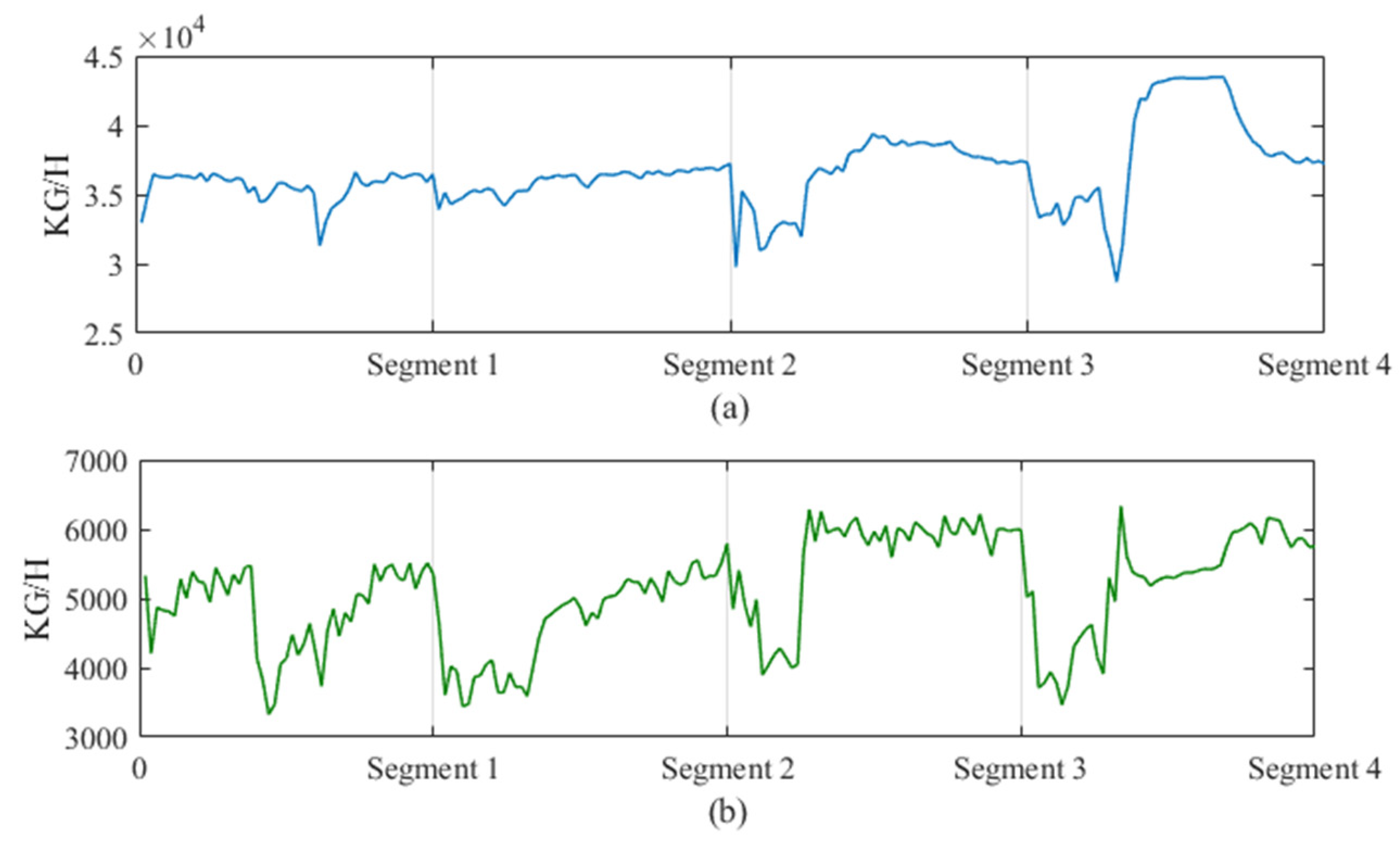
A situation involving materials, equipment, and complex connections often leads to the anomaly state of the textile process, resulting in shutdowns and accidents. Therefore, accurate anomaly detection is an essential part [26]. During textile production, we collected four segments of data with anomaly status for training purposes. These four data segments contain 200 sampling points.
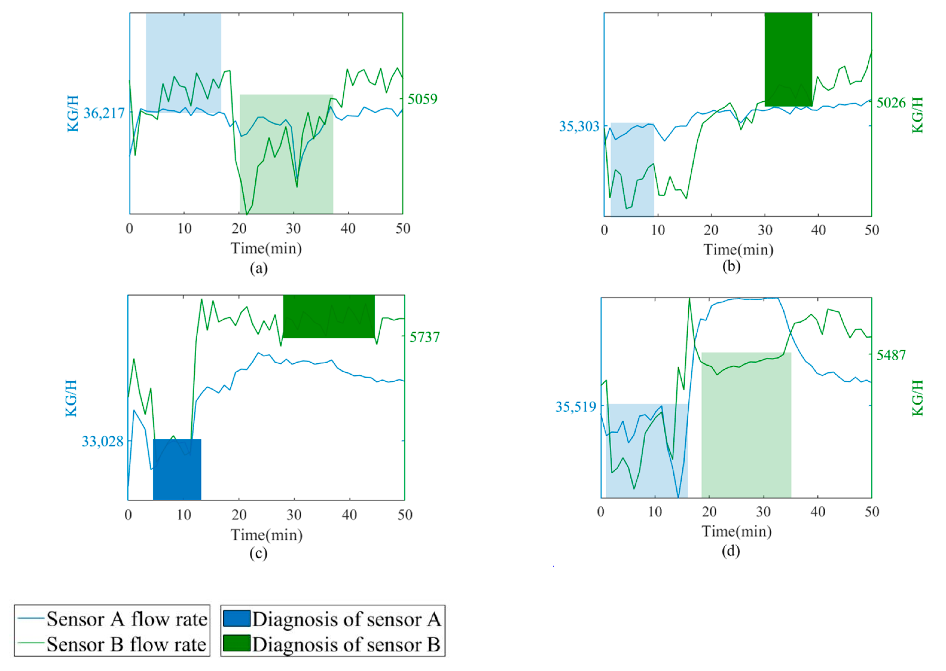
Figure 4 is the anomaly data, Figure 4a is the BHET flow rate at 200 sampling points from Sensor A, and Figure 4b is the BHET flow rate from Sensor B. We divide the observed data into intervals for every 50 sampling points. Four semantic anomaly detection formulas can be obtained using the offline learning model to design a semantic anomaly detector:
ϕ a = 0,50 ( 3,18 ( x 1 > 36217 ) 20,39 ( x 2 < 5059 ) ) ϕ b = 0,50 ( 2,8 ( x 1 < 35303 ) 30,38 ( x 2 > 5026 ) ) ϕ c = 0,50 ( 5,12 ( x 1 < 33028 ) 29,44 ( x 2 > 5737 ) ) ϕ d = 0,50 ( 1,16 ( x 1 < 35519 ) 19,34 ( x 2 < 5487 ) )
where x 1 represents the BHET flow rate from Sensor A and x 2 represents the BHET flow rate from Sensor B.
The semantics of anomaly detection formulas can be parsed in Table 2. Each logical formula can be transformed into a corresponding natural language, which is more readable and does not require computational interpretation. The operators can adjust the operation processes according to the anomaly state semantic interpretation.
Figure 5 is the result of visualization through the generated logical formulas. The blue region represents the variable x 1 and the green region represents x 2 . The lighter colour indicates the operator and the darker colour indicates the operator. The variable x 1 implicates the variable x 2 and the appearance of the green region, which leads to the blue region.
Through the HSTL learning of fault data, we can finally create a characteristic diagram of system anomaly representation (Figure 6). It is called a semantic anomaly detector (SeAD). The proposed classifier can be used for online anomaly detection of the textile process. When data are missing, the existing signal temporal logic model [8] cannot perform semantic anomaly detection. Figure 7 shows a case in which data are missing. The red interval represents the missing data.
ϕ e = 0,50 ( @ 20 ( 2,8 x 1 < 35303 30,38 x 2 > 5026 ) )
The formula reads “From 0 to 50, the flow rate from Sensor A is lower than 35,303 at least once within the time 2 to 8, resulting in the flow rate from Sensor B being higher than 5026 all the time from 30 to 38, but the data is missing at time 20”.
Our semantic hybrid signal temporal logic model can express the sequential data in more detail. The obtained semantic anomaly detection results have improved our understanding of the material changes in the pipeline when the anomaly occurs, which will help the operators regulate the process and make decisions.

4.3. Comparison of Experimental Results

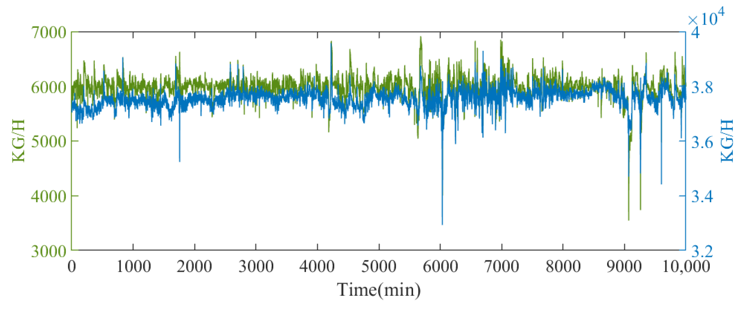
We collected 10,000 pairs of data as test sets. Due to the redundancy of the time-series data in the textile process, combined with the characteristics expressed by the logic formula, we segmented the data by 50 time points, and then 10,000 pairs of training data were divided into 200 segments.
Figure 8 shows the flow rate data from sensor A (blue) and sensor B (green) generated after the compound passes through the stirred tank during the melt transfer stage of polymer production.
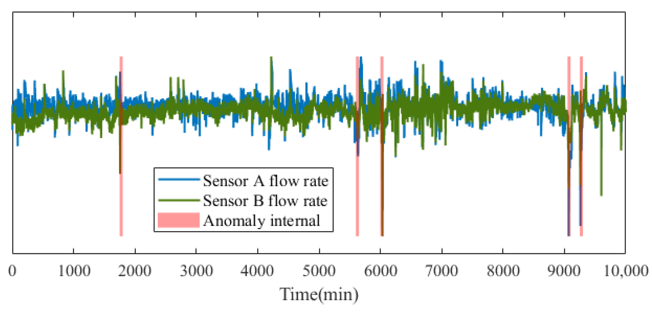
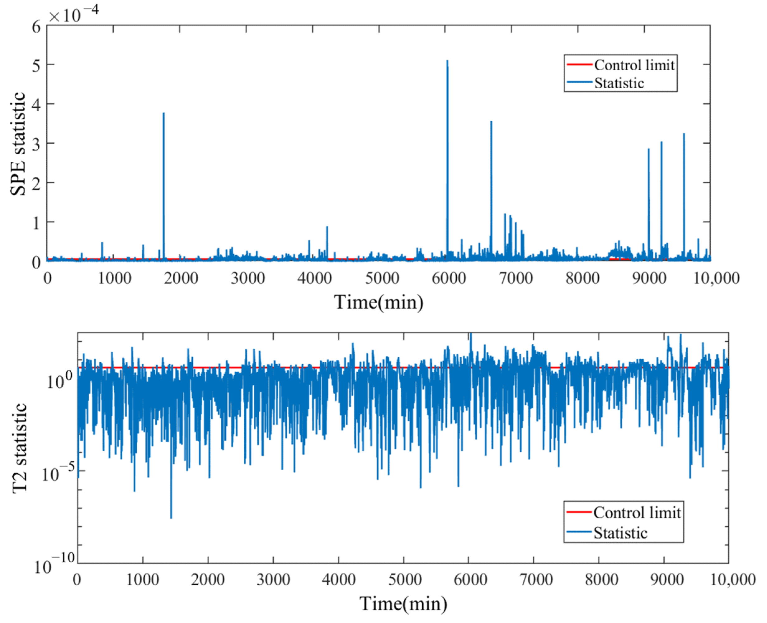
Figure 9 shows the experimental results of HSTL anomaly detection. The red interval represents the detected anomaly. The simulated annealing (SA) is used to optimize the robustness function ρ . The comparative experiments contain three representative methods: principal component analysis (PCA), the long-short term memory (LSTM) model, and the temporal logic-based method [15]. As a traditional statistical model, PCA remains relatively effective [17]. LSTM is a neural network model, which exhibits excellent feature extraction performance. A total of 5000 sampling points are selected as training data. The PCA method is based on T2 monitoring statistics and SPE monitoring statistics with a 95% control limit. The results are shown in Figure 10.
The precision, recall rate, and F1 value were selected as the performance evaluation indicators, and the results are shown in Table 3.
The F1 value demonstrates that the proposed method is feasible and has advantages compared with some existing methods. Among the existing methods for processing time series data, neural network-based models have advantages over statistical models. However, they require a lot of pre-training. Our proposed method has high accuracy and does not need a large number of training samples.

4.4. Ablation Analyses

In order to prove the validity of our model, the ablation analysis was carried out by different robustness function optimization methods. Figure 11a depicts the results of optimizing the robustness function using particle swarm optimization (PSO). Figure 11b depicts the results of optimizing the robustness function using a genetic algorithm (GA).
The precision, recall rate, and F1 value are shown in Table 4. The GA-based model has the highest accuracy but is the most time-consuming. By comparing the experiments using PSO and GA, we can verify the effectiveness of the HSTL model. As a result, no matter how the optimization method is chosen, it is superior to other models, indicating that our proposed model helps more in anomaly detection.

4.5. Semantic Anomaly Detector Transfer Detection

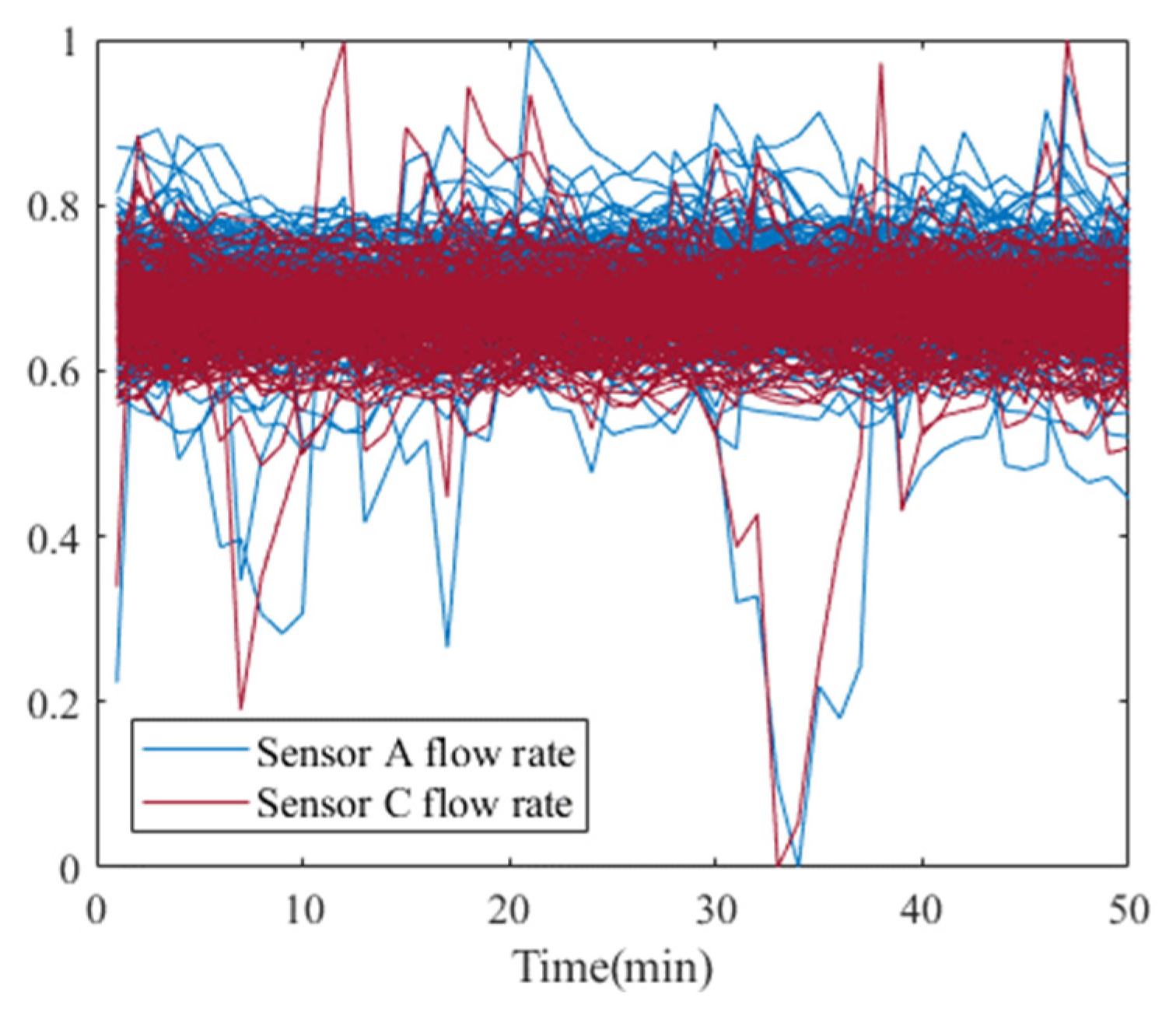
We acquired a semantic anomaly detector (Figure 6) from the time-series data obtained via Sensor A and Sensor C. The red lines represent the data comes from Sensor C. The data in Sensors A, B, and C have a strong correlation; therefore, detectors trained on data from Sensors A and B can be transferred to process Sensor C. We normalized the values in the detector obtained in Section 4.3. The four sets of formal formulas are as follows.
ϕ e = 0,50 ( 3,18 ( x 1 > 0.5090 ) 20,39 ( x 2 < 0.5760 ) ) ϕ f = 0,50 ( 2,8 ( x 1 < 0.4473 ) 30,38 ( x 2 > 0.5650 ) ) ϕ g = 0,50 ( 5,12 ( x 1 < 0.2936 ) 29,44 ( x 2 > 0.8015 ) ) ϕ h = 0,50 ( 1,16 ( x 1 < 0.4619 ) 19,34 ( x 2 < 0.7184 ) )
Figure 12 shows the time series data obtained from Sensors A and C, which were segmented and normalized. The result of semantic anomaly detection is shown in Figure 13. The experimental results show that the colored areas effectively cover the abnormal data.
From these experimental results and illustrations, we observe that the proposed algorithm can generate an anomaly detector that can effectively monitor the textile process. The variance of samples before and after the detection is used as the evaluation index, and the results are shown in Table 5. The variance of the tested data has been significantly reduced, illustrating the effectiveness of our model. The variance is defined as Equation (6), in which xi is the sample x ¯ is the average value n is the number of samples.
V a r = i = 1 n ( x i x ¯ ) 2 n
The semantic description of A C processes achieved via anti-normalization of the values in formulas ϕ e to ϕ h is shown in Table 6. The semantics can help operators effectively adjust working conditions. As shown here, the model proposed on the unlabeled dataset can still provide effective detection.

5. Conclusions

The temporal logic research object is an epistemic system based on the formalization of two intuitive concepts of proof and calculation, which mathematically studies the problems of reasoning and proof. The focus of data mining using temporal logic is on helping the machine to understand the meaning of symbols and helping it to learn logical formulas. Logical formulas are a kind of data feature that can be read and understood by humans. Based on the hybrid signal temporal logic, we propose a method of learning the logical relationship between two time-series data and use the learned relationship as a label to detect the textile process. The experimental results demonstrate the effectiveness of this method.
The data features learned according to the temporal logic method are interpretable. Since the semantic temporal logic system has a certain theoretical basis, it is unnecessary to use a large number of data to complete the training process. The difficulty of the temporal logic method lies in the complexity of the theory and modeling; these factors require further exploration.

Author Contributions

Conceptualization, X.H.; methodology, X.H.; software, X.H.; validation, K.H., formal analysis, K.H.; investigation, K.H.; resources, X.H.; data curation, X.H.; writing—original draft, K.H.; writing—review and editing, X.H.; visualization, X.H.; supervision, K.H.; project administration, K.H.; funding acquisition, K.H. All authors have read and agreed to the published version of the manuscript.

Funding

This research was funded by the National Key Research and Development Plan from Ministry of Science and Technology (2016YFB0302701), National Natural Science Foundation of China (no. 61903078), Natural Science Foundation of Shanghai (19ZR1402300, 20ZR1400400), Fundamental Research Funds for the Central Universities and Graduate Student Innovation Fund of Donghua University (CUSF-DH-D-2020081).

Data Availability Statement

The data that support the findings of this study are available on request from the corresponding author, RD.

Conflicts of Interest

The authors declare no conflict of interest.

References

  1. He, C.; Zhang, C.; Bai, T.; Jiao, K.; Su, W.; Wu, K.; Su, A. A Review on Artificial Intelligence Enabled Design, Synthesis, and Process Optimization of Chemical Products for Industry 4.0. Processes 2023, 11, 330. [Google Scholar] [CrossRef]
  2. Zhang, Z.; Zhao, J. A deep belief network based fault diagnosis model for complex chemical processes. Comput. Chem. Eng. 2017, 107, 395–407. [Google Scholar] [CrossRef]
  3. Kumar, A.; Jaiswal, A. A Deep Swarm-Optimized Model for Leveraging Industrial Data Analytics in Cognitive Manufacturing. IEEE Trans. Ind. Inform. 2021, 17, 2938–2946. [Google Scholar] [CrossRef]
  4. Su, A.; Zhang, C.; She, Y.-B.; Yang, Y.-F. Exploring Deep Learning for Metalloporphyrins: Databases, Molecular Representations, and Model Architectures. Catalysts 2022, 12, 1485. [Google Scholar] [CrossRef]
  5. Yasenjiang, J.; Xu, C.; Zhang, S.; Zhang, X. Fault Diagnosis and Prediction of Continuous IndustrialProcesses Based on Hidden Markov Model-BayesianNetwork Hybrid Model. Int. J. Chem. Eng. 2022, 2022, 3511073. [Google Scholar] [CrossRef]
  6. Yan, L.; Peng, X.; Tone, C.; Luo, L. A Multigroup Fault Detection and Diagnosis Scheme for Multivariate Systems. Ind. Eng. Chem. Res. 2020, 59, 20767–20778. [Google Scholar] [CrossRef]
  7. Hatamleh, M.; Chong, J.W.; Tan, R.R.; Aviso, K.B.; Janairo, J.I.B.; Chemmangattuvalappil, N.G. Design of mosquito repellent molecules via the integration of hyperbox machine learning and computer aided molecular design. Digit. Chem. Eng. 2022, 3, 100018. [Google Scholar] [CrossRef]
  8. Jian, C.; Yang, K.; Ao, Y. Industrial fault diagnosis based on active learning and semi-supervised learning using small training set. Eng. Appl. Artif. Intel. 2021, 104, 104365. [Google Scholar] [CrossRef]
  9. Kourtis, G.; Kavakli, E.; Sakellariou, R. A Rule-Based Approach Founded on Description Logics for Industry 4.0 Smart Factories. IEEE Trans. Ind. Inform. 2019, 15, 4888–4899. [Google Scholar] [CrossRef]
  10. Chen, G.; Liu, M.; Kong, Z. Temporal-Logic-Based Semantic Fault Diagnosis with Time-Series Data From Industrial Internet of Things. IEEE Trans. Ind. Electron. 2021, 68, 4393–44035. [Google Scholar] [CrossRef]
  11. Huo, X.; Hao, K.; Chen, L.; Tang, X.; Wang, T.; Cai, X. A dynamic soft sensor of industrial fuzzy time series with propositional linear temporal logic. Expert Sys. Appl. 2022, 201, 117176. [Google Scholar] [CrossRef]
  12. Pnueli, A. The temporal semantics of concurrent programs. Theoretical Comput. Sci. 1981, 13, 45–60. [Google Scholar] [CrossRef]
  13. Bringsjord, S. The logicist manifesto: At long last let logic-based artificial intelligence become a field unto itself. J. Appl. Logic. 2008, 6, 502–525. [Google Scholar] [CrossRef]
  14. Bartocci, E.; Gol, E.A.; Haghighi, I.; Belta, C. A formal methods approach to pattern recognition and synthesis in reaction diffusion networks. IEEE Trans. Control Netw. Syst. 2018, 5, 308–320. [Google Scholar] [CrossRef]
  15. Kong, Z.; Jones, A.; Belta, C. Temporal logics for learning and detection of anomalous behavior. IEEE Trans. Autom. Control. 2017, 62, 1210–1222. [Google Scholar] [CrossRef]
  16. Bombara, G.; Vasile, C.I.; Penedo, F.; Yasuoka, H.; Belta, C. A decision tree approach to data classification using signal temporal logic. In Proceedings of the ACM International Conference on Hybrid Systems: Computation and Control (HSCC), Vienna, Austria, 12–14 April 2016; pp. 1–10. [Google Scholar]
  17. Liu, K.; Lin, H.; Fei, Z.; Liang, J. Spatially–temporally online fault detection using timed multivariate statistical logic. Eng. Appl. Artif. Intell. 2017, 65, 51–59. [Google Scholar] [CrossRef]
  18. Kong, Z.; Jones, A.; Ayala, A.M.; Gol, E.A.; Belta, C. Temporal logic inference for classification and prediction from data. In Proceedings of the ACM International Conference on Hybrid Systems: Computation and Control (HSCC), Philadelphia, PA, USA, 15–17 April 2014; pp. 273–282. [Google Scholar]
  19. Gabbay, D.M.; Guenthner, F. Handbook of Philosophical Logic, 2nd ed.; Springer Publishing: New York, NY, USA, 2014; p. 62. [Google Scholar]
  20. Blackburn, P.; Tzakova, M. Hybrid Languages and Temporal Logic. Logic J. IGPL 1999, 7, 27–54. [Google Scholar] [CrossRef]
  21. Prior, A.N.; Hasle, P.F.V. Papers on Time and Tense; Oxford University Press: Oxford, UK, 2003; pp. 93–171. [Google Scholar]
  22. Brauner, T. Hybrid Logic and Its Proof-Theory; Springer Publishing: New York, NY, USA, 2001; pp. 21–56. [Google Scholar]
  23. Trinh, C.; Meimaroglou, D.; Hoppe, S. Machine Learning in Chemical Product Engineering: The State of the Art and a Guide for Newcomers. Processes 2021, 9, 1456. [Google Scholar] [CrossRef]
  24. Marin, C.; Popescu, D.; Petre, E. Modeling and Control of the Orthogonalization Plants in Textile Industry. IEEE Trans. Ind. Appl. 2019, 55, 4247–4257. [Google Scholar] [CrossRef]
  25. Jian, N.L.; Zabiri, H.; Ramasamy, M. Data-Based Modeling of a Nonexplicit Two-Time Scale Process via Multiple Time-Scale Recurrent Neural Networks. Ind. Eng. Chem. Res. 2022, 61, 9356–9365. [Google Scholar] [CrossRef]
  26. Jieyang, P.; Kimmig, A.; Dongkun, W.; Niu, Z.; Zhi, F.; Jiahai, W.; Liu, X.; Ovtcharova, J. A systematic review of data-driven approaches to fault diagnosis and early warning. J. Intell. Manuf. 2022, 1–28. [Google Scholar] [CrossRef]
  27. Deng, X.; Tian, X. A new fault isolation method based on unified contribution plots. In Proceedings of the 30th Chinese Control Conference, Yantai, China, 22–24 July 2011; pp. 4280–4285. [Google Scholar]
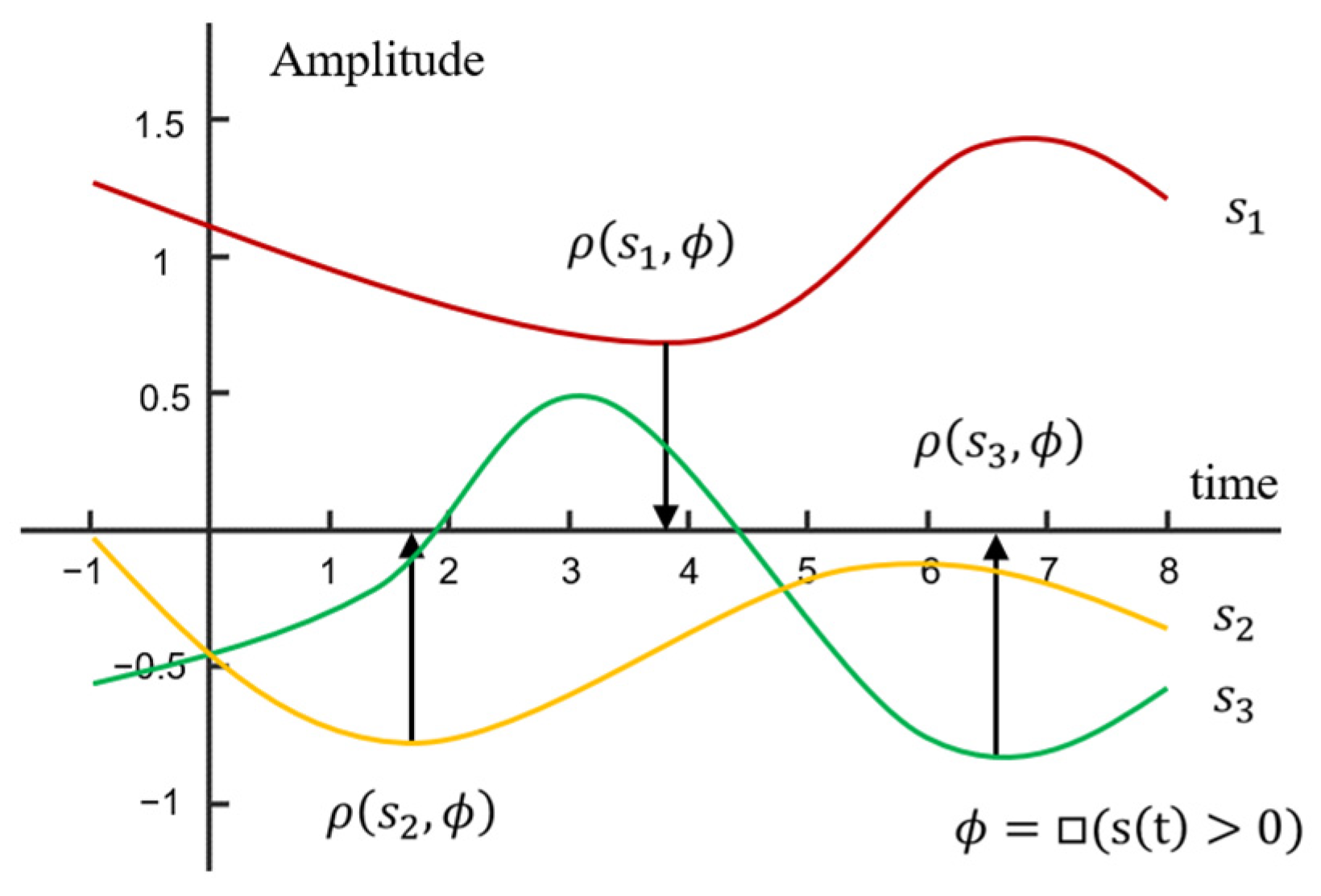
Figure 1. Robustness degrees for different series with formula ϕ .
Processes 11 02804 g001
Figure 2. The calculation process of the HSTL anomaly detection.
Processes 11 02804 g002
Figure 3. Polymerization process.
Processes 11 02804 g003
Figure 4. Flow rate data: (a) sensor A; (b) sensor B.
Processes 11 02804 g004
Figure 5. (a) visualization of formula ϕ a ; (b) visualization of formula ϕ b ; (c) visualization of formula ϕ c ; (d) visualization of formula ϕ d .
Processes 11 02804 g005
Figure 6. Semantic anomaly detector.
Processes 11 02804 g006
Figure 7. Missing data diagnosis.
Processes 11 02804 g007
Figure 8. Time-series data from sensor A and sensor B.
Processes 11 02804 g008
Figure 9. The detection result of HSTL.
Processes 11 02804 g009
Figure 10. The diagnosis result of PCA is based on SPE and T2.
Processes 11 02804 g010
Figure 11. The detection result of HSTL-based PSO (a) and GA (b).
Processes 11 02804 g011
Figure 12. Time-series data from Sensors A and C.
Processes 11 02804 g012
Figure 13. The detection of Sensors A and C.
Processes 11 02804 g013
Table 1. Literature review of temporal logic.
LiteratureApproachResult AchievedApplication Background
Kong et al. (2014) [18]Parameter signal temporal logic (PSTL)Discover temporal logic properties of a system from data.Herding
Synthetic biology
Kong et al. (2017) [15]Inference parametric signal temporal logic (iPSTL)Use data to construct a signal temporal logic (STL) formula that describes normal system behavior.Naval surveillance
Train braking system
Liu et al. (2017) [17]Timed multivariate statistical logic (TMSL)Specify not only spatial features but also temporal dynamics of systems in a formal manner.Robot arm system
Bartocci et al. (2018) [14]Tree-spatial superposition logic (TSSL)A formal framework for specifying, detecting, and generating spatial patterns in reaction–diffusion networks.Turing’s reaction–diffusion system
Chen et al. (2021) [10]Agenda-based, learning-enabled algorithmConstruct the formal specifications of faults directly from data collected from IIoT-enabled systems.Iron-making factory
Table 2. Semantic formulas for semantic anomaly detector.
FormulasSemantic Anomaly Detection
ϕ a From 0 to 50, the flow rate from Sensor A is higher than 36,217 at least once from time 3 to 18; as a result, the flow rate from Sensor B is lower than 5059 at least once from time 20 to 39.
ϕ b From 0 to 50, the flow rate from Sensor A is lower than 35,303 at least once from time 2 to 8; as a result, the flow rate from Sensor B is higher than 5026 the entire time from 30 to 38.
ϕ c From 0 to 50, the flow rate from Sensor A is lower than 33,028 the entire time from 5 to 12; as a result, the flow rate from Sensor B is higher than 5737 the entire time from 29 to 44.
ϕ d From 3 to 50, the flow rate from Sensor A is lower than 35,519 at least once from time 1 to 16; as a result, the flow rate from Sensor B is lower than 5487 at least once from time 19 to 34.
Table 3. Comparison of the six methods of test results.
PrecisionRecallF1Rank
PCA (SPE)10.71380.83307
PCA (T2)10.79080.88326
Deng [27]0.98750.85460.91615
Huo [11]10.92450.96084
LSTM0.976010.98793
GRU0.982310.99112
HSTL0.99990.98290.99131
Table 4. Comparison of results based on different optimization algorithms.
PrecisionRecallF1Time (s)
HSTL with SA0.99990.98290.99135.17
HSTL with PSO0.99670.99040.99356.32
HSTL with GA10.98790.993922.57
Table 5. Comparison of the variance before and after detection.
VarianceDecrease
Before DetectionAfter Detection
Sensor A6204.24724.523.85%
Sensor C2906.31982.831.78%
Table 6. Semantic of stage A C processes.
FormulasSemantic Anomaly Detection
ϕ e From 0 to 50, the flow rate from sensor A is higher than 36,217 at least once from time 3 to 18; as a result, the flow rate from Sensor C is lower than 31,014 at least once from time 20 to 39.
ϕ f From 0 to 50, the flow rate from Sensor A is lower than 35,303 at least once within Time 2 to 8; as a result, the flow rate from Sensor C is higher than 30,950 the entire time from 30 to 38.
ϕ g From 0 to 50, the flow rate from Sensor A is lower than 33,028 the entire time from 5 to 12; as a result, the flow rate from Sensor C is higher than 32,330 the entire time from 29 to 44.
ϕ h From 3 to 50, the flow rate from Sensor A is lower than 35,519 at least once from time 1 to 16; as a result, the flow rate from Sensor C is lower than 31,845 at least once from time 19 to 34.
Disclaimer/Publisher’s Note: The statements, opinions and data contained in all publications are solely those of the individual author(s) and contributor(s) and not of MDPI and/or the editor(s). MDPI and/or the editor(s) disclaim responsibility for any injury to people or property resulting from any ideas, methods, instructions or products referred to in the content.