Study on Flow Characteristics of a Single Blade Breakage Fault in a Centrifugal Pump

Abstract

The precise identification of faults in centrifugal pumps is crucial for ensuring their safe and stable operation, given their significance as vital industrial equipment. This article aims to rigorously examine and analyze the flow characteristics of centrifugal pumps under two specific conditions: normal blade operation and a single blade breakage fault. Through systematic comparison and in-depth study, this article sheds light on distinguishing flow patterns exhibited by these pumps under both normal and fault scenarios. Utilizing validated numerical simulation methods, a thorough analysis is conducted to explore the flow condition and energy characteristics of the impeller channel following the breakage of a single blade. Additionally, the article investigates changes in the pressure pulsation characteristics of the pump volute as a result. The numerical simulation results reveal that the head of the centrifugal pump decreases at all flow points when a single blade breaks. However, there is no significant change in efficiency at small flow points. As the flow rate exceeds 0.9Q_d, efficiency experiences a substantial decrease. Furthermore, the efficiency decline becomes even more pronounced as the flow rate continues to increase. At 1.5Q_d, efficiency plummets by 14.33%. The flow pattern undergoes significant changes as well. The breakage of the blade induces noteworthy secondary flow in adjacent impeller channels, resulting in heightened turbulence dissipation. Additionally, it was observed that blade fracture causes alterations in the main frequency of pressure pulsation within the volute. This is characterized by an increase in shaft passing frequency and a decrease in blade passing frequency. Notably, near the tongue monitoring point, the shaft frequency escalates by over 20 times.

1. Introduction

As a widely used rotating equipment, centrifugal pumps play an important role in the transportation of fluids [1,2]. In order to adapt to diverse lifestyle rhythms and ensure the stable operation of industrial processes, strict requirements have been imposed on the long-term stable operation of pumps in various pumping scenarios [3,4]. However, in the actual application process, due to their harsh working environment, pumps are inevitably prone to failures [5,6]. Blade breakage is one of the common faults in centrifugal pumps, and its unstable operation is closely related to flow characteristics such as reflux and pressure pulsation inside the pump [7,8]. Therefore, in order to accurately diagnose blade breakage faults and shorten the maintenance cycle of centrifugal pumps, it is very important and necessary to explore the flow characteristics after faults occur [9].

Previous research on the fault diagnosis of centrifugal pumps mainly focused on the extraction of fault features and the study of diagnostic algorithms. Ahmad et al. [10] presents a centrifugal pump fault diagnosis framework based on supervised contrastive learning. The framework employs a convolutional neural network model to extract vibration signal features and trains the model using a contrastive loss function to make samples of the same fault closer in the feature space while separating samples of different faults. Zaman et al. [11] presents a novel approach for centrifugal pump fault diagnosis using a SobelEdge scalogram and convolutional neural networks. Chen et al. [12] presents a centrifugal pump fault diagnosis method based on current signals and an analysis approach for cavitation using soft measurement techniques, demonstrating high accuracy and reliability. N.R. Sakthivel et al. [13] compares different dimensionality reduction techniques for fault diagnosis of mono block centrifugal pumps using vibration signals. In the research conducted by Araste et al. [14], a thorough investigation was carried out on impeller tip failure, cracking, leakage, and cavitation in a centrifugal pump. Their experiments provided valuable insights into the behavior of these faults and their impact on the pump’s performance. Similarly, Jamimoghaddam et al. [15] employed self-organizing maps in their study to detect three specific faults (impeller tip failure, impeller cracking failure, and cavitation) as well as inefficient operating points during testing. The results of their experiments demonstrated the effectiveness of their proposed method in accurately identifying anomalies in centrifugal pump operation. These findings contribute to a better understanding of the faults that can occur in centrifugal pumps and provide a foundation for developing effective monitoring and maintenance strategies.

Cao et al. [16] proposes a combination of principal component analysis and the Gaussian mixture model to effectively identify blade crack faults in centrifugal pumps. Experimental data of normal and cracked blade conditions was collected, and PCA was employed to reduce the dimensionality of the feature space. GMM was then utilized to model the normal and fault conditions to classify the blade crack faults. Wu et al. [17] and Tan et al. [18] discuss investigation of the performance of a centrifugal pump with a broken impeller and multi-malfunction (broken blade and seal ring abrasion). Tests and numerical simulations were conducted to analyze the energy characteristics, vibration, internal flow, pressure pulsation, and radial force of the pump. Zhai et al. [19] focuses on four scenarios for marine centrifugal pumps: the normal state, the initial stages of a fault, the intermediate stages of a fault, and the late stages of a fault. They employ the delayed detached eddy simulation technique with a non-linear eddy viscosity model to calculate the hydrodynamic characteristics of the pump in its broken state. The objective was to gain insights into the pump’s performance under different conditions, examining external characteristics, flow patterns, pressure pulsations, and flow analysis.

Despite extensive research on diagnosing faults in centrifugal pumps, the majority of studies have concentrated on extracting fault features and developing diagnostic algorithms, while there has been limited investigation into blade breakage faults. In previous studies concerning blade breakage faults, the primary emphasis has been on extracting fault features like vibration, while neglecting to investigate the flow state following the occurrence of blade fracture faults. This approach fails to effectively utilize alterations in flow characteristics for the identification of vibration and other fault features. This study focuses on investigating the fault of a single blade fracture in a single-stage centrifugal pump. Numerical simulations are conducted and validated through experiments to analyze and compare various aspects, including external characteristics, internal flow and pressure distribution, energy characteristics, blade loading characteristics, and pressure pulsation before and after blade fracture. The findings from this research serve as a valuable basis and reference for diagnosing single blade breakage faults in centrifugal pumps.

2. Blade Breakage Fault

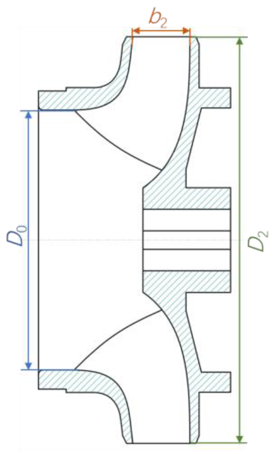
2.1. Test Pump

This article focuses on the research of single-stage single-suction centrifugal pump. It follows the acceptance test procedure for water pump model and device model, as stated in the water conservancy industry standard of the People’s Republic of China SL 140–2006. To conduct the test, a scaled-down version of the centrifugal pump prototype, in a ratio of 2:5, was designed. The specific conversion process is presented below [20]:

$$Q_{\mathrm{P}} = Q_{\mathrm{M}}\left(\frac{n_{\mathrm{P}}}{n_{\mathrm{M}}}\right){\left(\frac{D_{\mathrm{P}}}{D_{\mathrm{M}}}\right)}^3$$

(1)

$$H_{\mathrm{P}} = H_{\mathrm{M}}{\left(\frac{n_{\mathrm{P}}}{n_{\mathrm{M}}}\right)}^2{\left(\frac{D_{\mathrm{P}}}{D_{\mathrm{M}}}\right)}^2$$

(2)

where, Q_P is the flow rate of the prototype pump, Q_M is the flow rate of the test pump, n_P is the rotational speed of the prototype pump, n_M is the rotational speed of the model pump, D_P is the impeller diameter of the prototype pump, D_M is the impeller diameter of the model pump, H_P is the head of the prototype pump, H_M is the head of the model pump.

The main designed parameters of the prototype pump and the test pump are shown in

Table 1. The comparison of main performance parameters between the prototype pump and the test pump.

Parameters	Q (m3/h)	H (m)	n (r/min)	ns
prototype pump	3800	43	985	220
test pump	363	15.3	1470	220

.

The impeller geometrical parameters of the prototype centrifugal pump are shown in Figure 1. The value of each parameter of the impeller is shown in

Table 2. The fundamental geometric characteristics of the original pump.

Geometric Characteristics	Value
The quantity of blades on the impeller	6
The impeller’s outlet diameter/mm	660
The impeller’s outlet width/mm	90
The impeller’s inlet width/mm	440

.

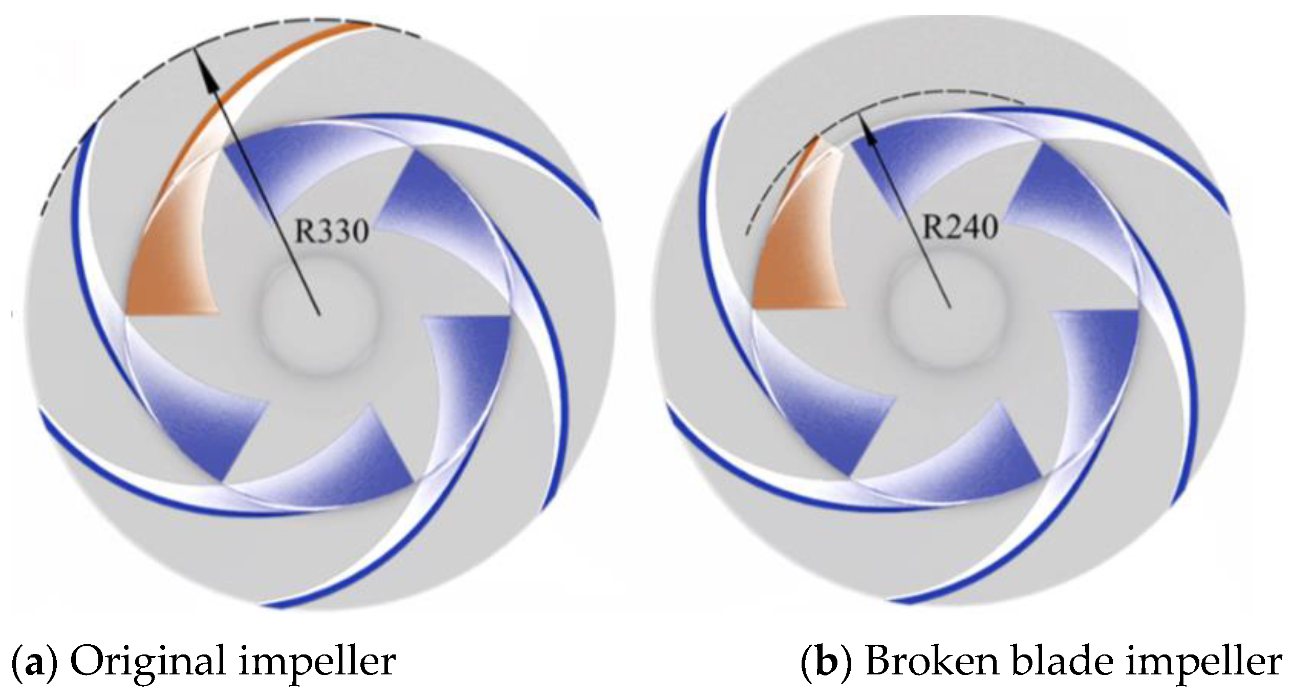
2.2. Blade Breakage Fault Mode

Figure 2 shows the breakage fault mode. The original blade radius was 330 mm, and the blade breakage fault occurred on a single blade of the impeller. The radius after breakage was 240 mm, and the length of the broken blade was approximately 0.5 times the original blade length.

3. Experiment and Numeral Calculation

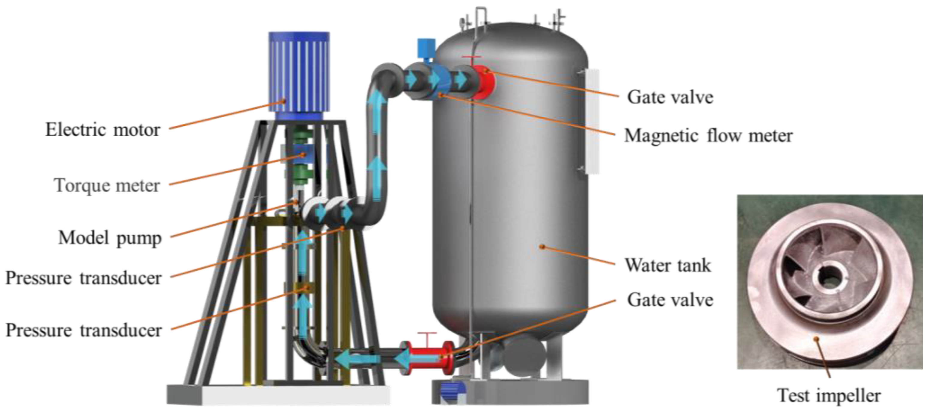
3.1. Design of Experimental Setup

The test pump was fabricated in accordance with the design parameters’ proportions for the purpose of testing and verification. Figure 3 shows the schematic diagram of the experimental setup. The test equipment mainly includes a model pump, an electric motor, inlet and outlet gate valves, a water tank, a magnetic flow meter, a pressure transducer, a torque meter, etc. During the experiment, the head, speed, and torque of the model pump at different flow rates were obtained by adjusting the outlet valve, and data collection was conducted after the centrifugal pump was stable in operation.

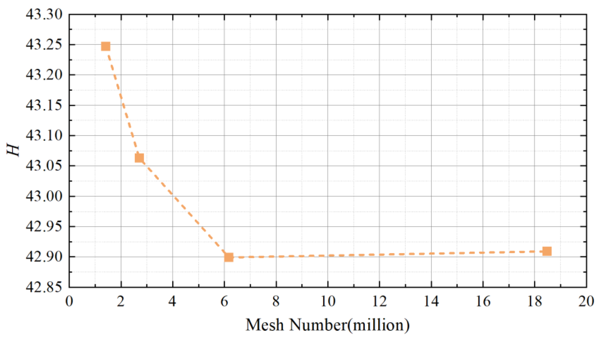
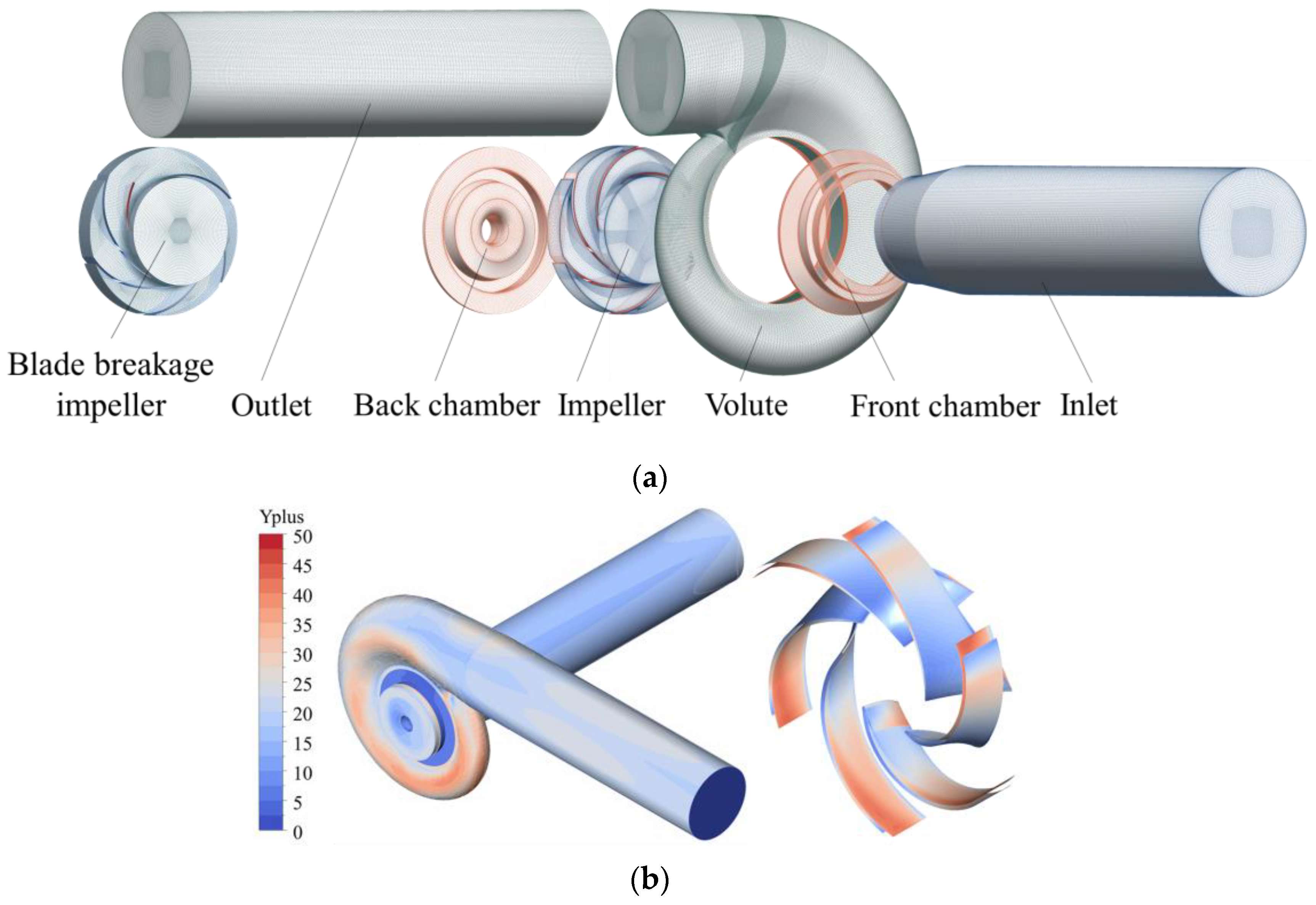
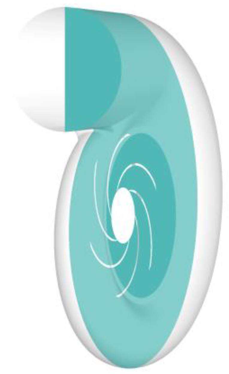
3.2. Hydraulic Model Components and Meshing

The 3D calculation model of the test pump is depicted in Figure 4, consisting of: Inlet, Impeller, Volute, Outlet, Front chamber, and Back chamber.

The usage of the commercial software ICEM 2021R2 enables the meshing of the model, allowing for the implementation of a structured grid that can effectively enhance the density and number of nodes in the boundary layer. This feature is particularly advantageous in areas of intricate flow, such as the impeller and volute regions. In order to minimize the solution error caused by the number of grids, four different sets of grid schemes were generated for independent verification, as illustrated in

Table 3. The mesh number of the centrifugal pump.

Section	Inlet	Impeller	Volute	Front Chamber	Back Chamber	Outlet	Total
Mesh Number	248,937	219,078	707,818	47,656	91,200	101,910	1,416,599
	537,681	674,832	1,238,111	90,712	117,496	47,658	2,706,490
	538,692	1,183,896	1,982,208	1,049,880	747,912	675,000	6,177,588
	2,239,545	4,529,616	4,522,624	2,239,545	3,492,480	14,61,257	18,485,067

. The independent verification parameters were focused on the head H of the centrifugal pump, considering the pump’s design conditions. The results reveal that when the total number of water grids in the model pump exceeds 6,177,588, the fluctuation of the pump head value becomes negligible, indicating satisfactory grid independence, as is shown in Figure 5. In the present study, in order to enhance the accuracy and intricacy of the internal flow field analysis within the impeller, a more refined mesh was employed, with particular emphasis placed on refining the internal mesh within the impeller. As a result, the total number of grids in the final mesh reached 18.48 million, which can be observed in Figure 6, depicting the mesh model.

3.3. The Setting of Boundary Conditions

The ANSYS CFX 2020R1 software was utilized to perform a steady simulation in this study. To accurately simulate the turbulent behavior, the shear stress transport (SST) k-ω turbulence model was employed. This widely accepted turbulence model has been extensively validated in various industrial applications [21]. The SST k-ω turbulence model provides high accuracy when predicting eddy formations under high strain rates. The working fluid used was water at a temperature of 25 °C, with a density of 997 kg/m³ and a kinematic viscosity of 8.899 × 10⁻⁴ kgm⁻¹s⁻¹. The outlet boundary condition, as depicted in Figure 4, was set to represent normal speed outlet, while the inlet boundary condition was defined as the average static pressure inlet. Frozen rotor interfaces were employed to facilitate the exchange of physical parameters between interfaces. Near the wall surface, the standard wall function was applied, and the wall was treated as an adiabatic non-slip surface.

3.4. Experimental Verification

Figure 5 shows the pump performance curve under normal blade condition. At Figure 7, the pump performance curve of the pump measured by the test was in good agreement with the numerical results under the normal blade condition. The maximum error between experimental data and numerical data was less than 9%. This shows that the numerical data matches well with the experimental data.

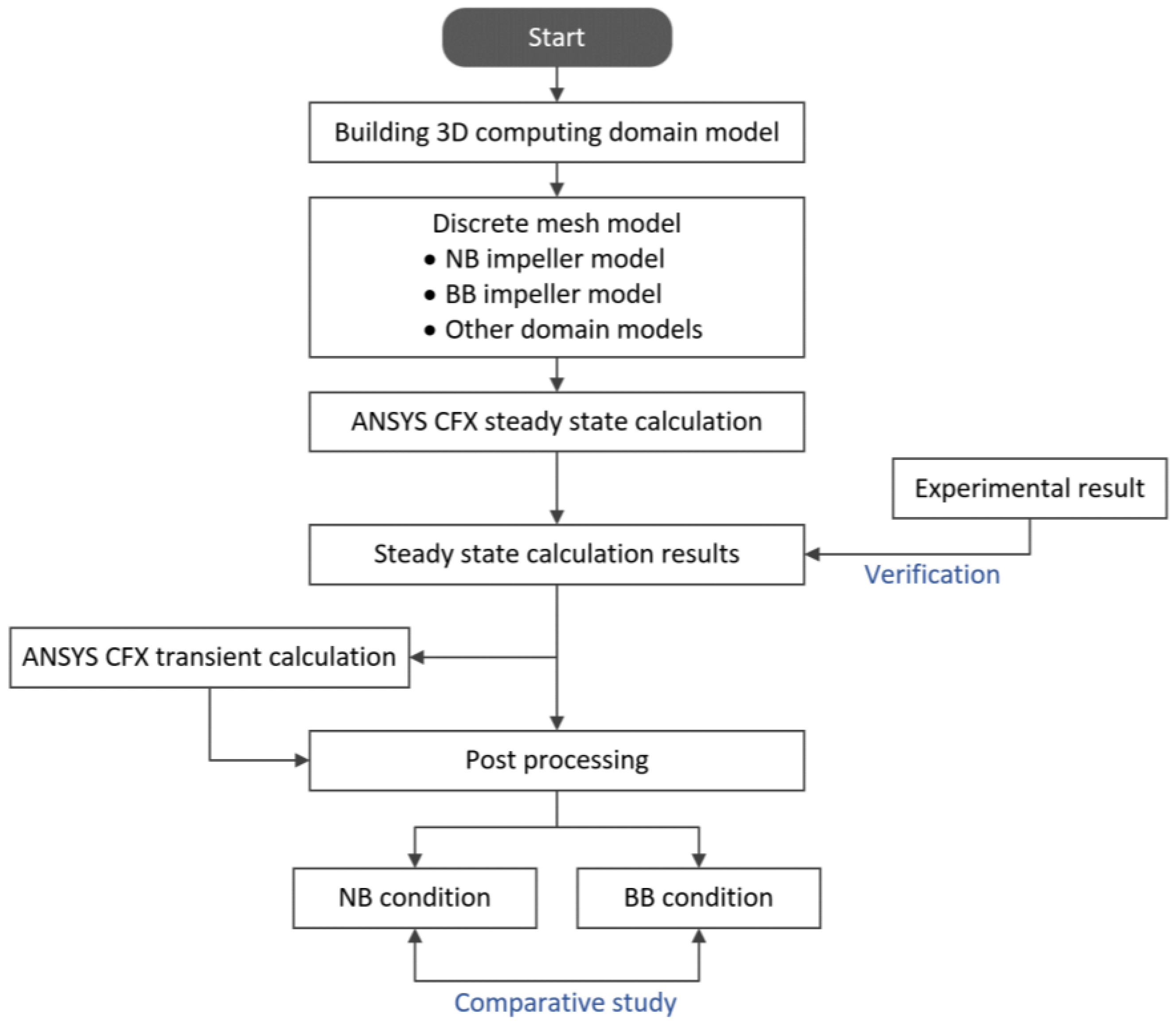
3.5. Flowchart of Numerical Simulations

The flowchart in Figure 8 illustrates the procedure for numerical calculations, and the numerical calculation process described in this article was derived from this flowchart.

4. Analysis of Results

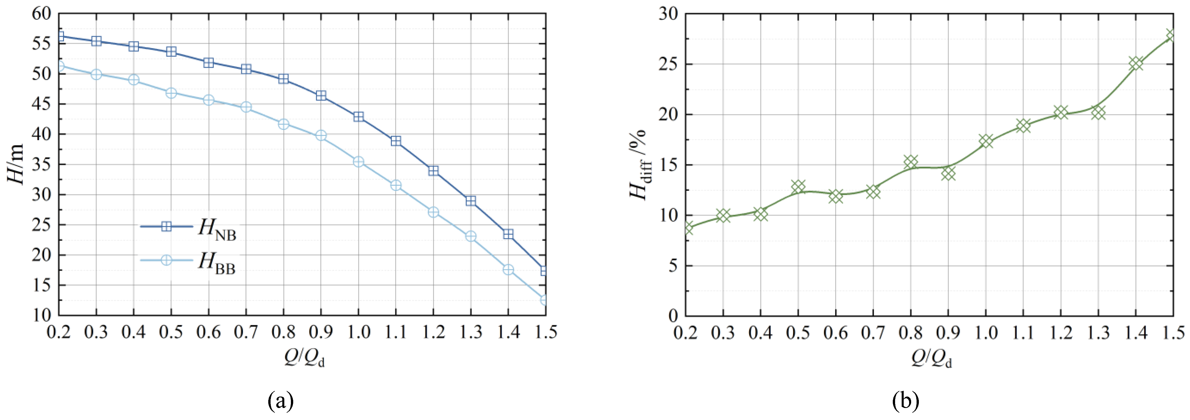
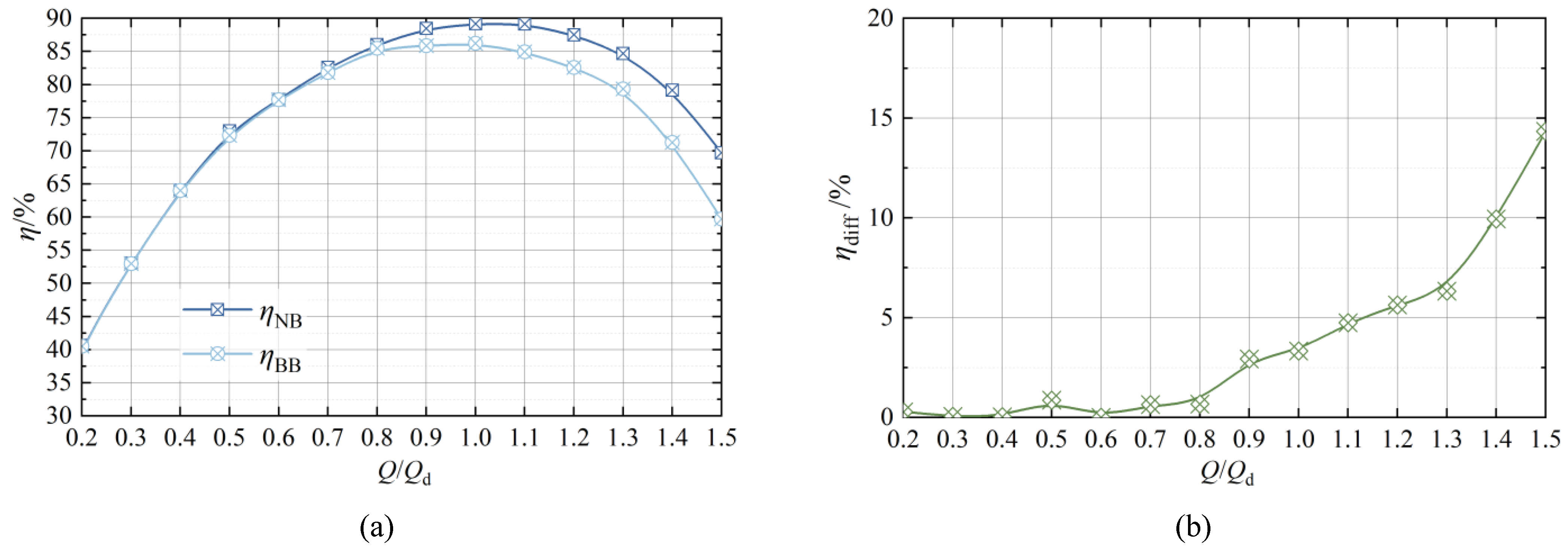
4.1. Transformations in Performance

Figure 9a shows the head flow curve of a centrifugal pump under the normal blade and blade breakage fault conditions. It can be seen from the figure that the change trend of the head with flow after blade breakage was completely consistent with that of normal impeller, and the head drop value of the centrifugal pump due to blade breakage at each flow point was close. As shown in Figure 9b, the proportion of head reduction caused by blade breakage at different flow points is shown. It can be seen from the figure that with an increase in flow rate, the proportion of head decline caused by blade breakage gradually increased, and the decline rate gradually increased, reaching the maximum value of 27.84% at 1.5Q_d.

Figure 10a shows the head efficiency curve of the heart pump under normal blade and blade breakage fault conditions. It can be seen from the figure that the effect of blade breakage on efficiency was not significant under small flow conditions, but the efficiency decreases significantly under large flow conditions, and the optimal efficiency point shifts to the small flow point. As shown in Figure 10b, the efficiency reduction ratio caused by blade breakage at different flow points is shown. It can be seen from the figure that the efficiency fluctuated only slightly in the small flow area. When the flow rate was greater than or equal to 0.9Q_d, the efficiency decreased significantly, and the proportion of decline increased, reaching the maximum value of 14.33% at 1.5Q_d.

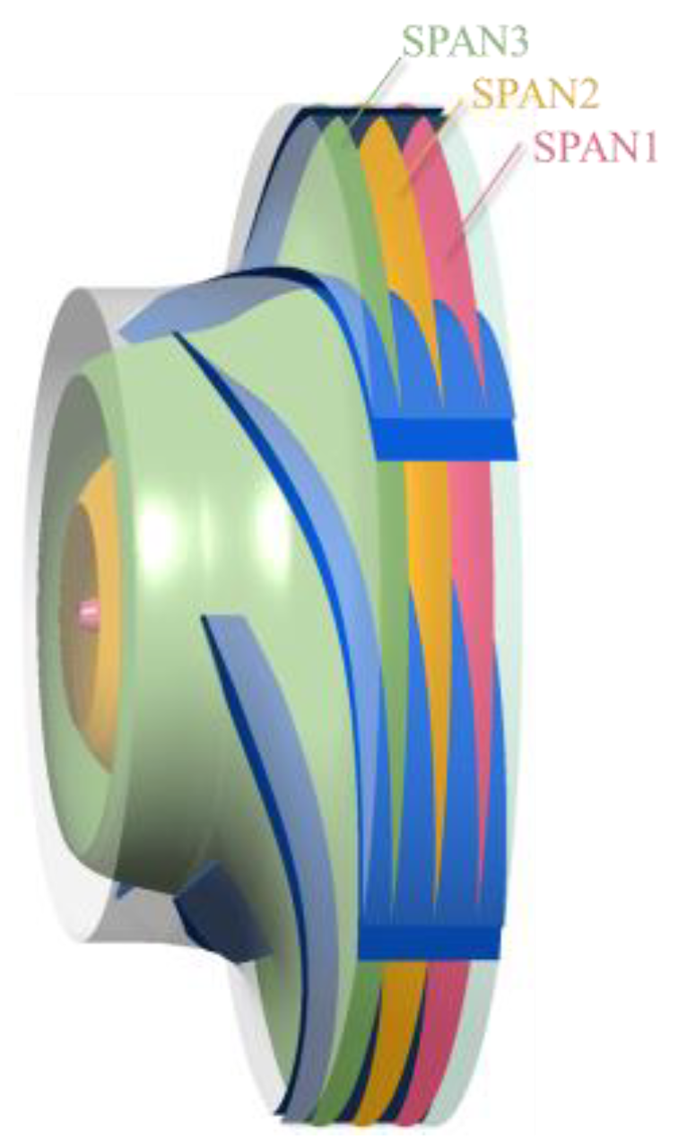
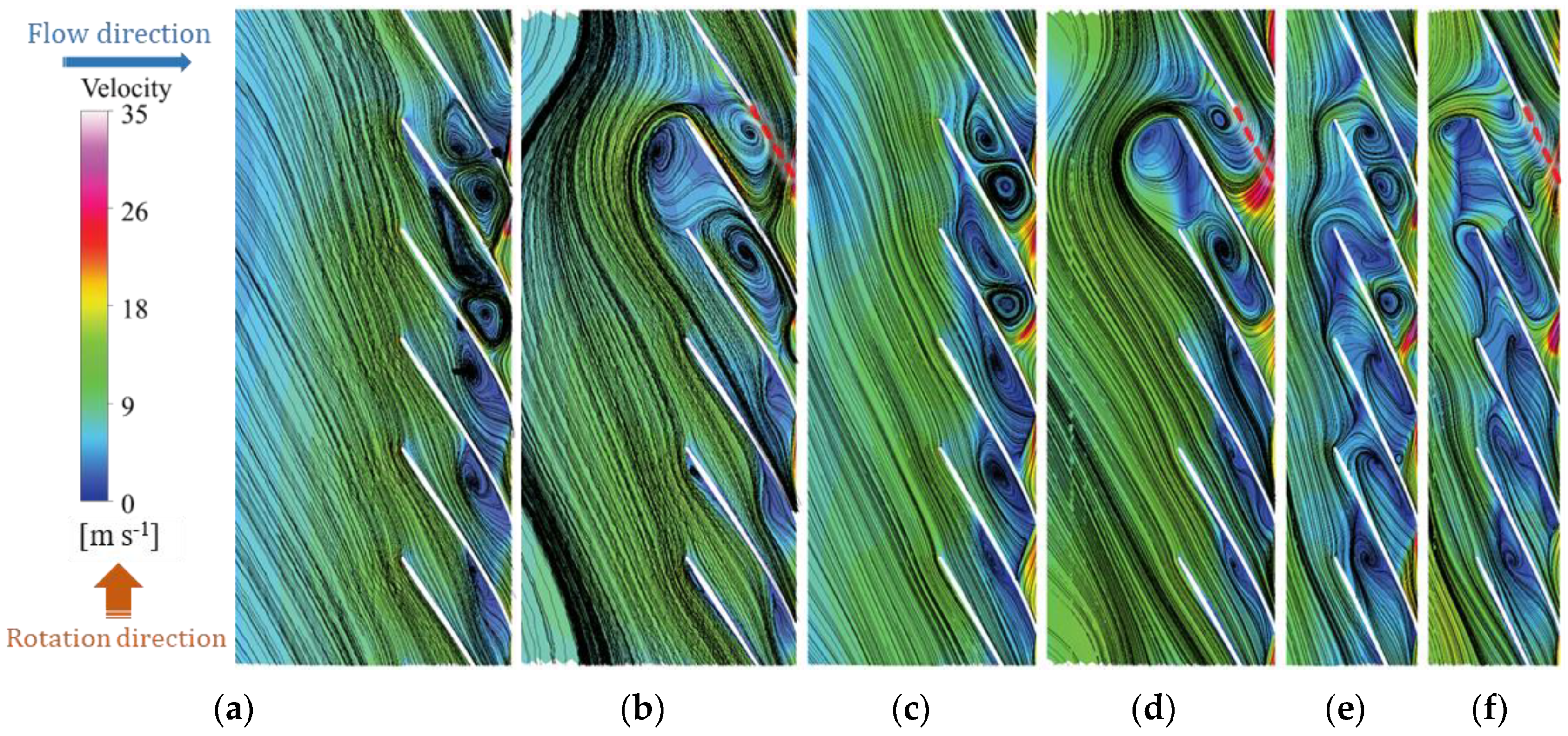
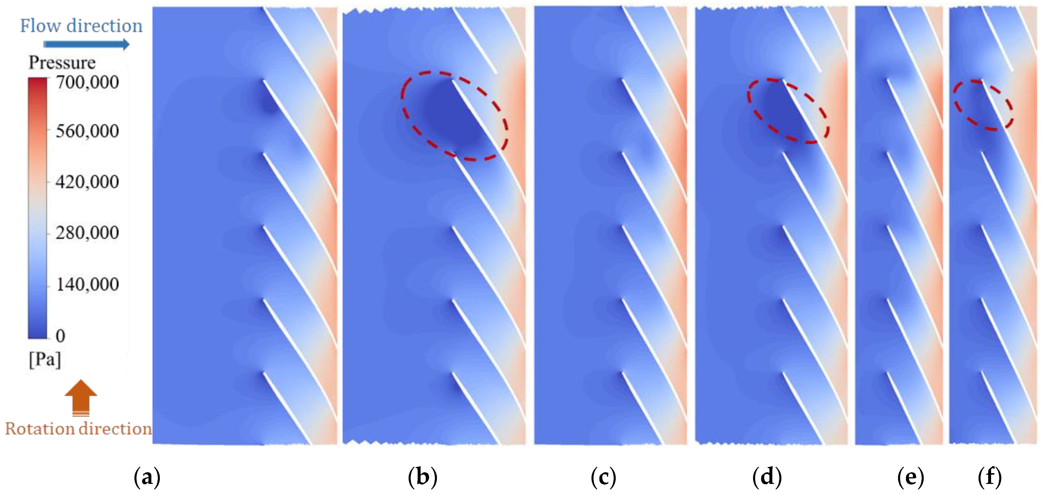
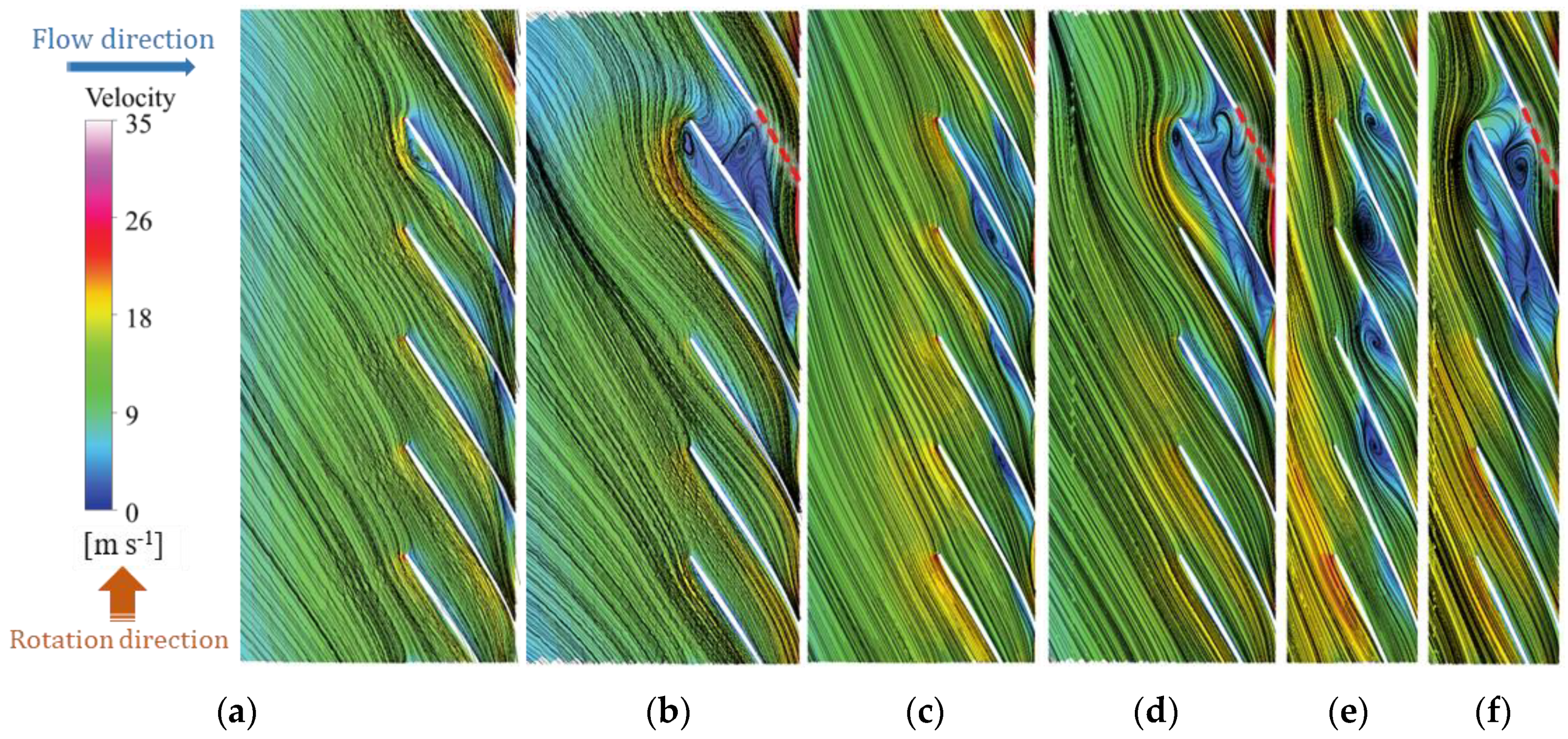
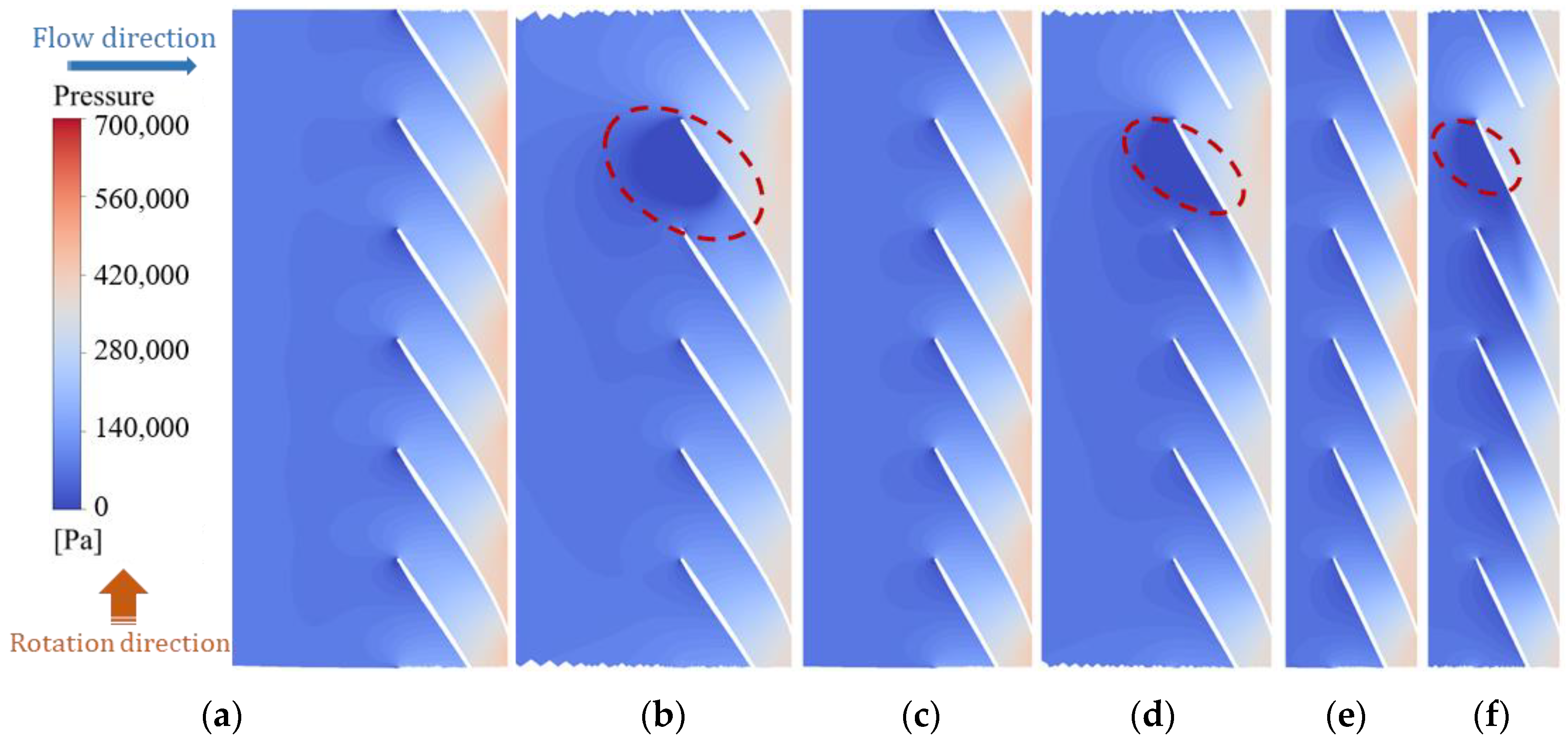
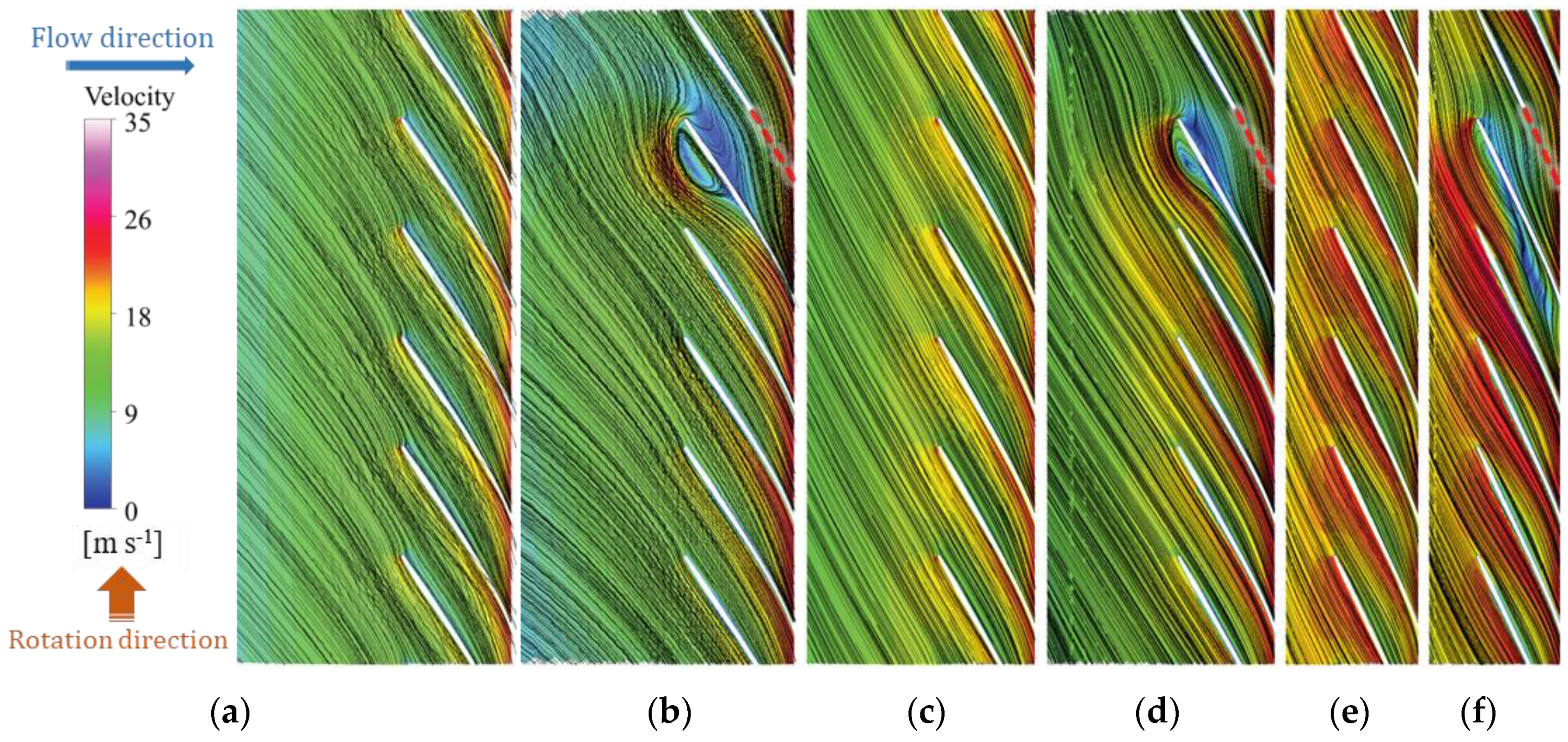
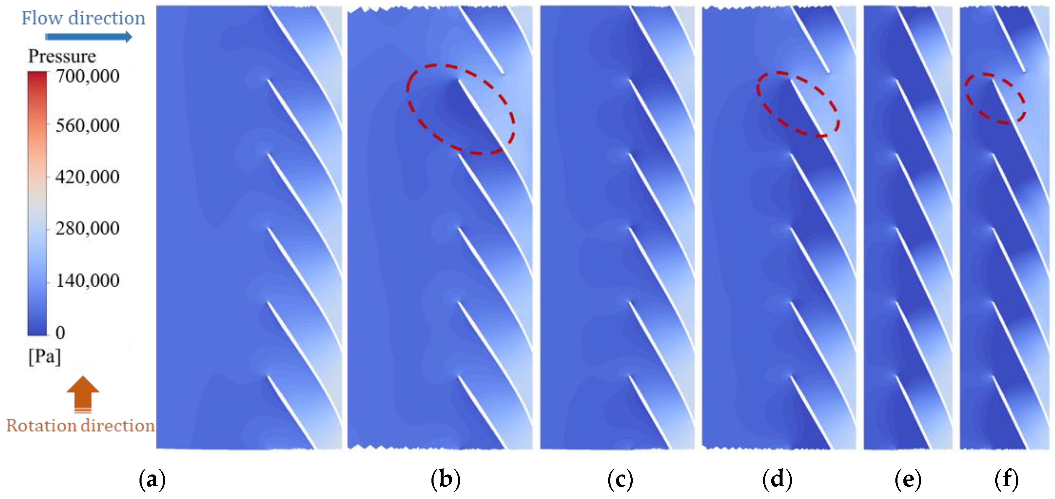
4.2. Span Surface Velocity and Pressure Analysis

To visually study the changes in the flow state inside the impeller after blade damage, SPAN1-3 was set inside the impeller, with corresponding span values of 0.2, 0.5, and 0.8, respectively, as is shown in Figure 11.

Figure 12 shows the pressure distribution on each span surface of 0.2Q_d. It can be seen from the figure that under normal blade conditions, the pressure distribution in each channel was uniform, and the pressure from inlet to outlet increased gradually. When the blade is damaged, the pressure in the suction surface passage of the damaged blade was obviously uneven, and a large low-pressure area appeared at the inlet of the next damaged blade. Figure 13 shows the velocity and streamline diagram of each span surface of 0.2Q_d. Under the low-flow condition, there was a large area of eddy current in each channel of the impeller, while under the blade damage condition, the influence range of the eddy current was large, which led to an eddy current before the blade inlet and affected the inlet flow of each channel.

In Figure 14, the pressure distribution diagram of each span surface of 0.6Q_d is shown. It can be seen from the figure that the pressure distribution in each channel under normal blade and broken blade conditions was similar to that in Figure 11. In Figure 15, the velocity and streamline diagram of each span surface of 0.6Q_d is shown. There are small area vortices in Span1 and Span2. In Span3, there is a large area of vortex under the normal blade to block the flow channel, while under the condition of a broken blade, the vortex affected the range of two flow channels, and the flow channels in other channels were in good condition, which was an unexpected phenomenon that the blade damage improved the flow state of the channel.

In Figure 16, the pressure distribution on each span surface of 1.0Q_d is shown. It can be seen from the figure that there was a low-pressure area near the inlet edge of the suction surface of the next blade from the broken blade, which is no different from the normal blade. In Figure 17, the velocity and streamline diagram of each span surface at 1.0Q_d is shown. The low-pressure positions of Span1, Span2, and Span3 of damaged blades correspond to large-area vortices, while the flow state of normal blades is excellent, and no vortex is visible.

In Figure 18, the pressure distribution of each span surface of 1.4Q_d is shown. It can be seen from the figure that different from other working conditions, there is no obvious low-pressure area due to the reduction of the head. It can also be seen in Figure 19 that there is no large-area vortex area in each span, except that there is a low-speed area at the inlet of Span2 and Span3 under the impact of incoming flow.

According to Figure 12, Figure 13, Figure 14, Figure 15, Figure 16, Figure 17, Figure 18 and Figure 19, under each span surface under the BB working condition, there is a reflux area at the inlet of the adjacent channel of the fractured blade, and the area corresponds to low pressure, as shown in the elliptical wireframe in the figures, but this phenomenon does not occur under the NB working condition. According to the streamline diagram, because the blade is broken under the BB working condition, the broken part lacks the restriction on the flow in the channel, causing the liquid to migrate to the next channel, affecting the normal flow of the original fluid in the next channel, and squeezing the fluid in this channel back into the inlet. Under the comprehensive effect, the flow in the adjacent channel was affected, and a large area of vortex appears. The energy loss at the vortex led to the low pressure at this position.

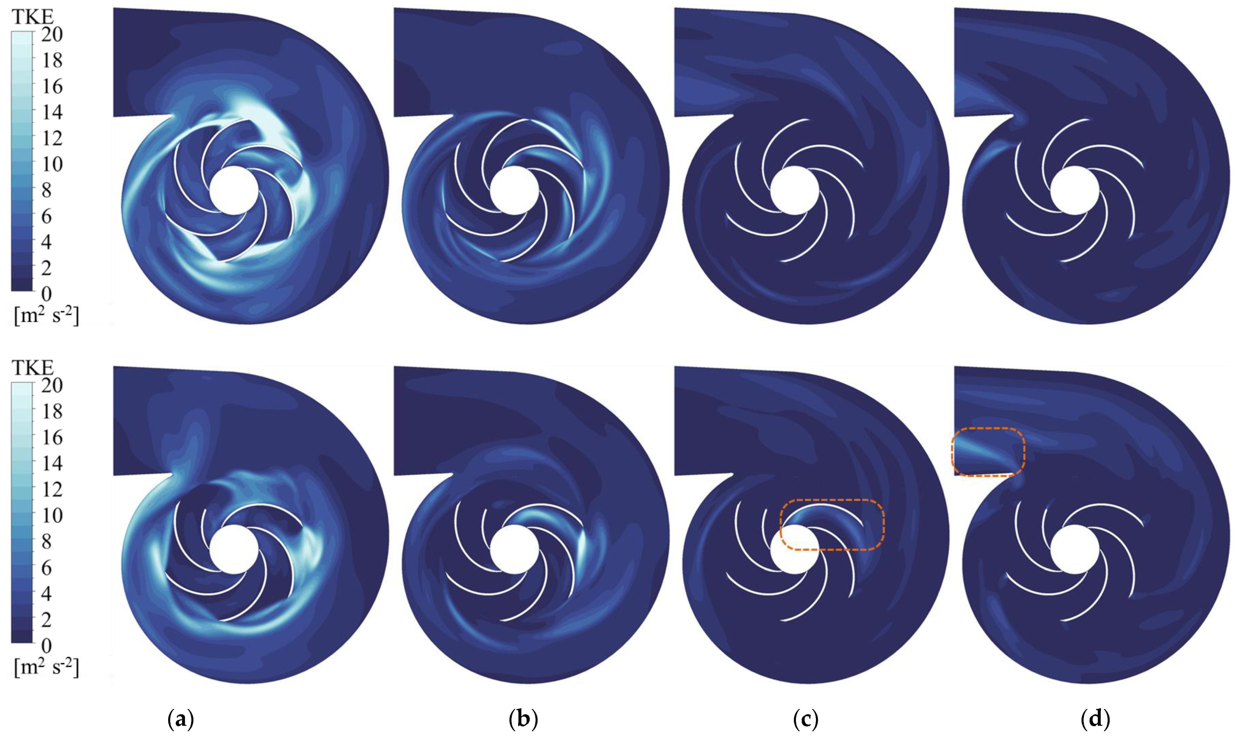
4.3. Turbulent Kinetic Energy Analysis

Although the blade breakage fault occurs in the impeller, the matching effect of the impeller and volute was equally important for the operation of the centrifugal pump. Therefore, the meridian plane was selected as shown in Figure 20. The turbulent kinetic energy of the meridian plane under the working conditions of 0.2Q_d~1.4Q_d was analyzed.

Turbulent kinetic energy represents the energy of turbulent motion in the fluid, that is, the higher the value of turbulent kinetic energy, the higher the turbulence intensity and the more intense the energy loss. The distribution of turbulent kinetic energy in the meridian plane of centrifugal pump under different working conditions is shown in Figure 21. Under the 0.2Q_d working condition shown in Figure 21a, the high turbulent kinetic energy dissipation zone was located at the impeller outlet, and the blade damage weakened the turbulent kinetic energy at the outlet. According to Figure 21b, when the flow rate increased to 0.6Q_d, the turbulent kinetic energy intensity in the impeller passage decreased, and the high-turbulent kinetic energy region further decreased. The distribution of turbulent kinetic energy at 1.0Q_d as shown in Figure 21c shows that, unlike the low-flow condition, the turbulent kinetic energy in the normal impeller was almost invisible at 1.0Q_d, while there was still a region with high-turbulent kinetic energy intensity in the broken blade impeller. Under the 1.4Q_d working condition shown in Figure 21d, the mismatch between the volute and the flow was much stronger than that of the impeller, and the high-turbulent kinetic energy dissipation zone mainly existed in the volute.

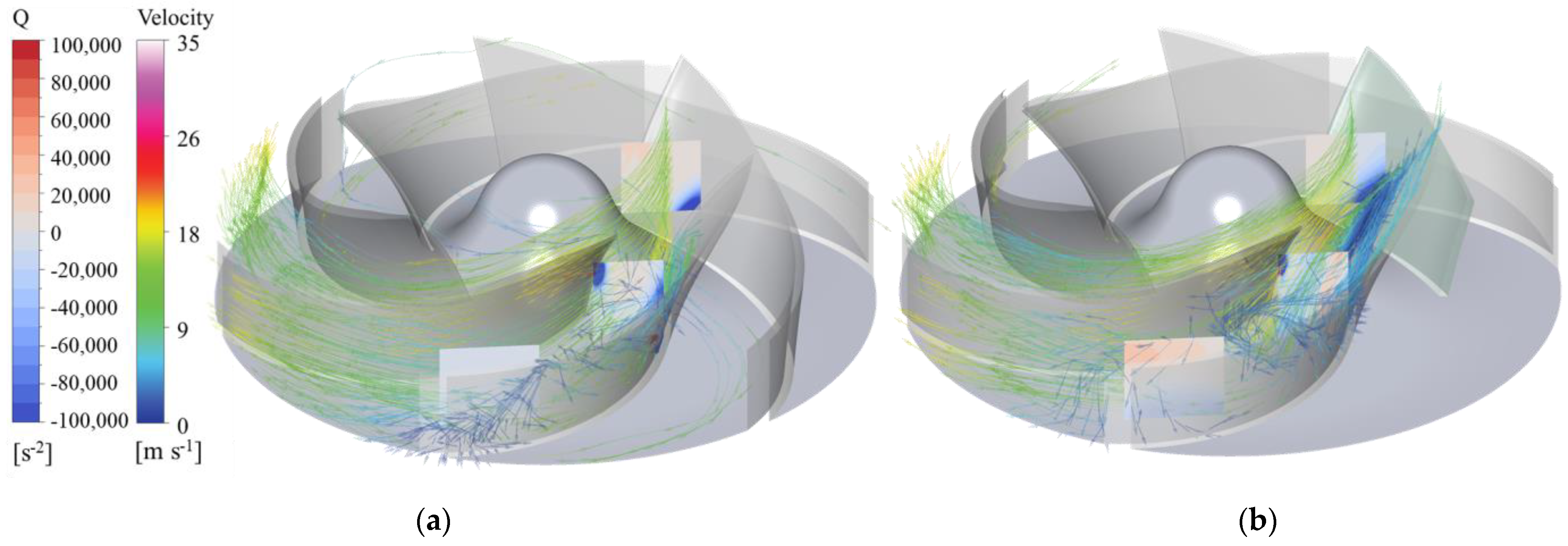
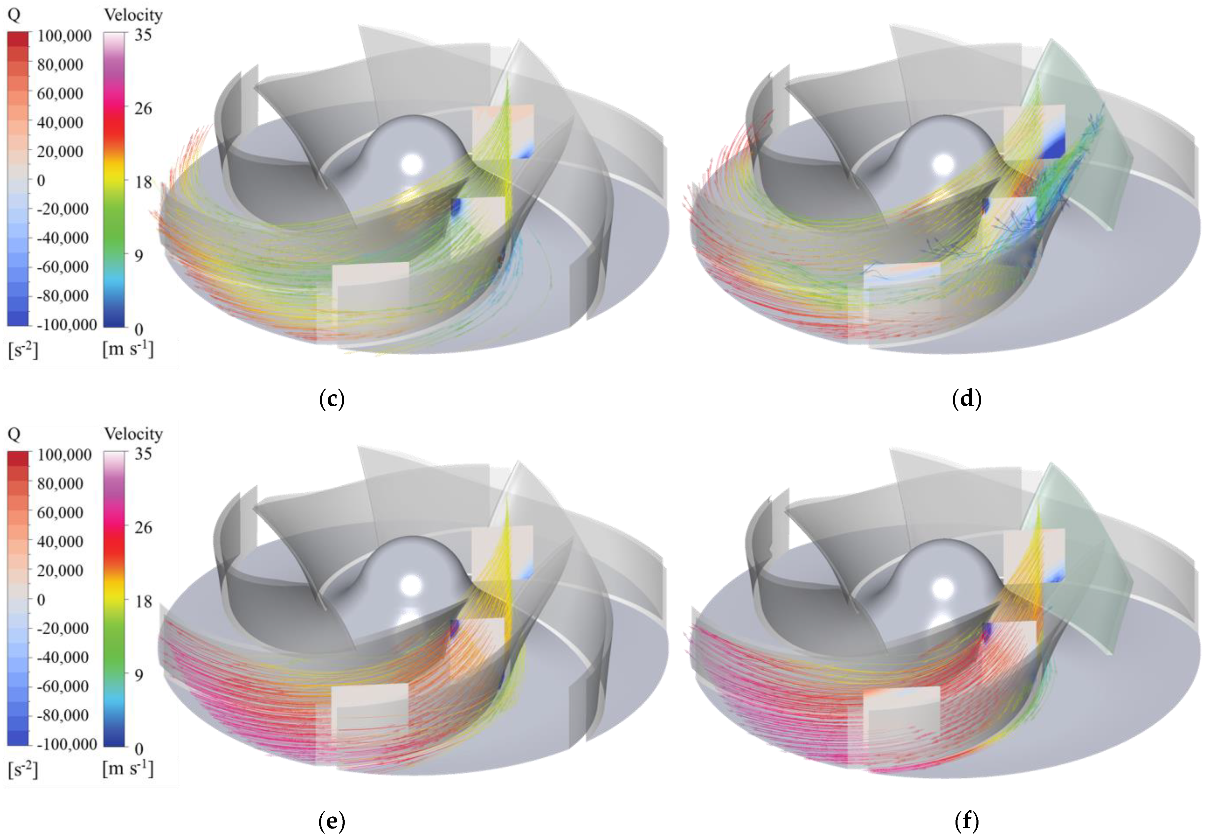
4.4. Vorticity Analysis in the Channel

In order to intuitively understand the low-pressure vortex structure in the adjacent channel of the damaged blade, show the streamline in the channel under different flow rates, and select the front, middle, and rear three planes of the channel to show the value of the plane Q criterion, as shown in Figure 22.

Compared with Figure 22a,b, under the working condition 0.6Q_d, there were multiple vortices near SS in the flow line in this channel, but it is obvious that the flow line vortex area in BB channel was larger and more noticeable. The value of the Q criterion on the plane also reflects this problem. Compared with Figure 22c,d, under the working condition 1.0Q_d, the streamline distribution in the channel in the NB condition was uniform, while there was a huge vortex near the inlet of the SS surface in the channel in the BB condition, which caused the fluid in the adjacent channel to be attracted into the channel. By comparing the values of the Q criteria of each plane, it can be concluded that there was only one region with an excessive strain rate near the wall under NB condition. However, under the BB condition, in addition to the larger area near the wall where the strain rate was too large, there was also a cross area where the strain rate in the channel was too large and the rotation intensity was too large. Compared with Figure 22e,f, the effect of broken blades on the flow state in the impeller at 1.4Q_d was small, and the effect caused by the mismatching of the inlet and outlet angles of the blades occupied the dominant position.

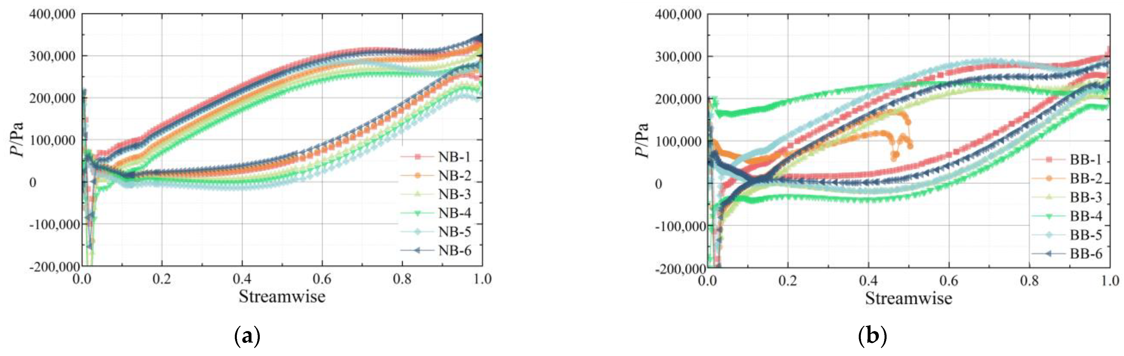
4.5. Comparison of Blade Loads

Blade load refers to the pressure difference between the SS and PS at the same position of the same blade, and its pressure distribution can be calculated from the flow field conditions.

The pressure distribution of SS and PS in NB and BB blades under 0.6Q_d is shown in Figure 23. It shows that the load distribution of each blade under a NB working condition is basically the same, and the maximum load position is in the middle of the blade. Under the BB condition, the load distribution of BB-2 and BB-6 blades is quite different from that of other blades. BB-2 is a broken blade, and its blade load is very small, while the maximum position of the BB-6 blade load appears in the front of the blade, which is different from the other blades. The pressure distribution of SS and PS of the NB and BB blades under 1.0Q_d is shown in Figure 24. It shows that the load distribution of each blade under the NB working condition is almost the same, and the maximum load position is still in the middle of the blade. Under the BB condition, the load of the BB-2 and BB-6 blades is still different from that of the other blades. BB-2 is a broken blade, and its pressure distribution on SS and PS surfaces is basically the same as that on PS surfaces of the other blades, while the maximum load position of the BB-6 blade appears in the front of the blade, and gradually decreases along the flow direction. The pressure distribution of SS and PS of the NB and BB blades at 1.4Q_d is shown in Figure 25. It shows that the load distribution of each blade under the NB working condition is similar, and the maximum load position is still in the middle of the blade. Under the BB condition, the load of the BB-2 and BB-4 blades is different from the other blades. BB-2 is a damaged blade, and the pressure distribution on the SS and PS surfaces of the BB-4 blade intersects and decreases at the damaged position, while the pressure at the PS surface inlet of the BB-4 blade is much higher than that of the other blades.

5. Transient Pressure Pulsations

5.1. Transient Calculation Method

In the process of transient numerical calculation, the time step for the rotor component to rotate 3° was set considering both calculation accuracy and calculation time. The data of 10 rotations was calculated, and the data of the last revolution was selected for analysis. With a rotational speed of 985 r/min, equivalent to a time step of 5.07614 × 10⁻⁴ s, the total calculation time was 0.60914 s. The steady-state numerical calculation results under the corresponding flow were taken as the initial values. The dynamic and static interfaces were then changed to transient rotor stator, and the convergence accuracy for the calculation was set to 10⁻⁵.

5.2. Monitoring Points

To explore the influence of blade breakage faults on the pressure pulsation characteristics in the pump, 18 uniformly distributed pressure pulsation monitoring points were set up in the volute, on the meridian plane, as shown in Figure 26. The pressure pulsation signals from the last rotation cycles of the numerical calculation results were processed and analyzed.

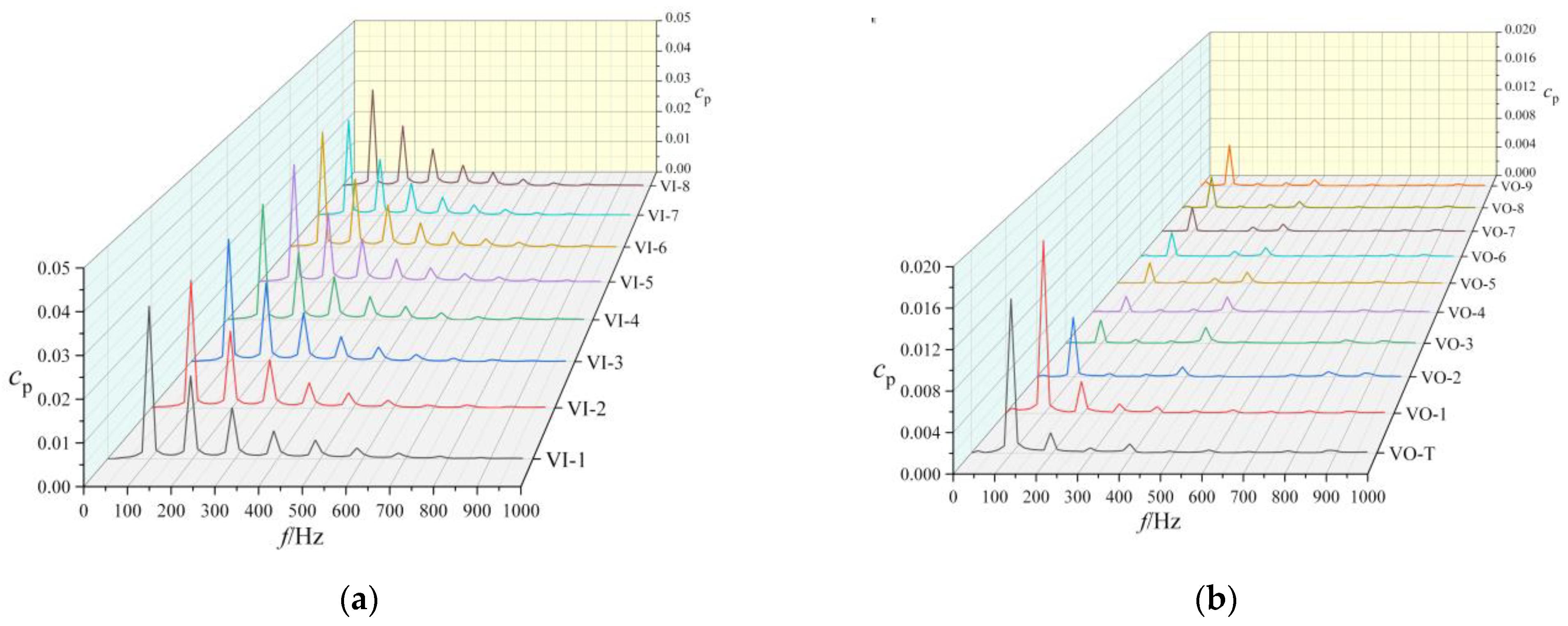
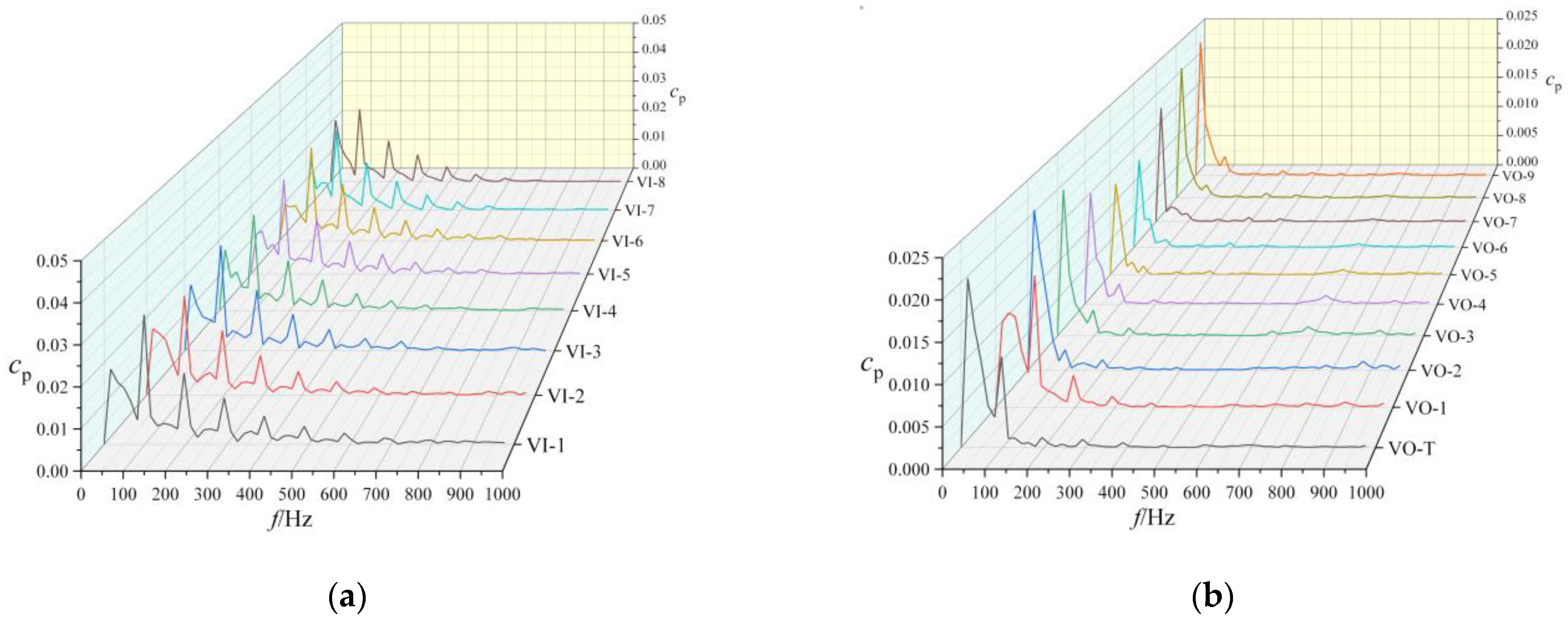
5.3. Pressure Pulsations

For the convenience of analysis, the pressure signal was non-dimensionalized and the pressure pulsation coefficient was defined as follows [22]:

$${\mathrm{c}}_P = \frac{P-P_{av}}{0.5\rho u_2^2}$$

(3)

In Equation (3), P is the pressure of the monitoring point; $P_{av}$ is the average pressure of the monitoring points; ρ is the water density; and $u_2$ is a constant value of 34.04 m/s.

As shown in Figure 27, the frequency domain diagram of pressure pulsation at monitoring points in the volute under the NB condition of 1.0Q_d is shown. It can be seen from Figure 27a that the dominant frequency at each point of VI is the blade passing frequency, and the difference in pressure pulsation intensity at each point of VI is small. It can be seen from Figure 27b that the main frequency of pulsation at each point of VO is also the blade passing frequency, in which VO-T and VO-1 have the largest amplitude at the blade passing frequency, mainly because these two points are closest to the dynamic and static interference surface, and the dynamic and static interference effect is the most obvious.

As shown in Figure 28, the frequency domain diagram of pressure pulsation at monitoring points in the spiral case under the BB working condition of 1.0Q_d is shown. It can be seen from Figure 28a that the main frequency at each point of VI is still the blade passing frequency, but compared with the NB working condition, the amplitude of the shaft passing frequency increased sharply with the increase in damage degree, and the change of speed of the shaft passing frequency at point VI-8 introduced the possibility of exceeding the blade passing frequency as the main frequency. It can be seen from Figure 28b that the dominant frequency at each point of VO was basically the axial frequency. Except for VO-T and VO-1, the amplitude of the blade passing frequency at other points was far less than the dominant frequency, which was also due to the obvious interference between the two points.

Figure 29 shows the pressure pulsation intensity of BPF and SPF at VO-1 and VO-T under the NB and BB conditions. It can be seen from the figure that the intensity of SPF under the NB condition was very low, while the intensity of SPF under the BB condition increased by more than 20 times, and the BPF decreased relatively. This feature can be used as one of the bases for judging blade breakage faults.

6. Conclusions

The purpose of this study was to analyze the flow characteristics of a centrifugal pump when a single blade is damaged. To achieve this, a numerical simulation was conducted and validated by experiments. Various parameters including performance curves, flow pattern, pressure distribution inside the impeller, turbulent kinetic energy, vorticity distribution, and pressure pulsation were compared between the conditions of normal and damaged blades. The findings provide valuable insights into the influence of damaged blades on the flow characteristics of centrifugal pump and fault diagnosis. The results can be summarized as follows:

(1)

After a broken blade failure, the head will drop under the same flow rate, but the efficiency is basically not affected under the condition of low flow rates. With the increase in flow rate, the proportion of efficiency reduction increases. Under the 1.5Q_d condition, the proportion of efficiency reduction increases to 14.33%.

(2)

When a single blade is broken, the change in the damaged blade channel is not obvious, but a large number of vortices appear at the inlet of the next channel, resulting in a large low-pressure area, affecting the flow in this channel.

(3)

Under normal working conditions, the main frequency of pressure pulsation at each monitoring point of the spiral case is BPF, while the intensity of SPF is very low. Under the condition of blade damage, the SPF intensity of pressure pulsation at each monitoring point of volute increases, and the BPF intensity decreases to a certain extent, especially at VO-T point, the SPF becomes the dominant frequency.

In the future investigations, the flow characteristics of a centrifugal pump can serve as valuable reference data for extracting fault features from other monitoring signals. They can be employed as a screening technique to differentiate between mechanical-induced fault features and fluid-induced fault features.

References

- Patra, J.; Pandey, N.K.; Muduli, U.K.; Natarajan, R.; Joshi, J.B. Hydrodynamic Study of Flow in the Rotor Region of Annular Centrifugal Contactors Using Cfd Simulation. Chem. Eng. Commun. 2013, 200, 471–493. [Google Scholar] [CrossRef]
- Stan, M.; Pana, I.; Minescu, M.; Ichim, A.; Teodoriu, C. Centrifugal Pump Monitoring and Determination of Pump Characteristic Curves Using Experimental and Analytical Solutions. Processes 2018, 6, 18. [Google Scholar] [CrossRef]
- Jia, X.; Chu, Q.; Zhang, L.; Zhu, Z. Experimental Study on Operational Stability of Centrifugal Pumps of Varying Impeller Types Based on External Characteristic, Pressure Pulsation and Vibration Characteristic Tests. Front. Energy Res. 2022, 10, 866037. [Google Scholar] [CrossRef]
- Wang, J.; Zhang, L.; Zheng, Y.; Wang, K. Adaptive prognosis of centrifugal pump under variable operating conditions. Mech. Syst. Signal Process. 2019, 131, 576–591. [Google Scholar] [CrossRef]
- Sunal, C.E.; Dyo, V.; Velisavljevic, V. Review of Machine Learning Based Fault Detection for Centrifugal Pump Induction Motors. IEEE Access 2022, 10, 71344–71355. [Google Scholar] [CrossRef]
- Yu, R.; Liu, J. Failure analysis of centrifugal pump impeller. Eng. Fail. Anal. 2018, 92, 343–349. [Google Scholar] [CrossRef]
- Wu, D.; Yao, S.; Lin, R.; Ren, Y.; Zhou, P.; Gu, Y.; Mou, J. Dynamic Instability Analysis of a Double-Blade Centrifugal Pump. Appl. Sci. 2021, 11, 8180. [Google Scholar] [CrossRef]
- Zhang, S.; Chen, H.; Ma, Z.; Wang, D.; Ding, K. Unsteady flow and pressure pulsation characteristics in centrifugal pump based on dynamic mode decomposition method. Phys. Fluids 2022, 34, 112014. [Google Scholar] [CrossRef]
- Yu, T.; Shuai, Z.; Jian, J.; Wang, X.; Ren, K.; Dong, L.; Li, W.; Jiang, C. Numerical study on hydrodynamic characteristics of a centrifugal pump influenced by impeller-eccentric effect. Eng. Fail. Anal. 2022, 138, 106395. [Google Scholar] [CrossRef]
- Ahmad, S.; Ahmad, Z.; Kim, J.-M. A Centrifugal Pump Fault Diagnosis Framework Based on Supervised Contrastive Learning. Sensors 2022, 22, 6448. [Google Scholar] [CrossRef] [PubMed]
- Zaman, W.; Ahmad, Z.; Siddique, M.F.; Ullah, N.; Kim, J.-M. Centrifugal Pump Fault Diagnosis Based on a Novel SobelEdge Scalogram and CNN. Sensors 2023, 23, 5255. [Google Scholar] [CrossRef] [PubMed]
- Chen, L.; Yan, H.; Xie, T.; Li, Z. Identification of cavitation state of centrifugal pump based on current signal. Front. Energy Res. 2023, 11, 1204300. [Google Scholar]
- Sakthivel, N.R.; Nair, B.B.; Elangovan, M.; Sugumaran, V.; Saravanmurugan, S. Comparison of dimensionality reduction techniques for the fault diagnosis of mono block centrifugal pump using vibration signals. Eng. Sci. Technol. Int. J. 2014, 17, 30–38. [Google Scholar] [CrossRef]
- Araste, Z.; Sadighi, A.; Moghaddam, M.J. Support Vector Machine-Based Fault Diagnosis of a Centrifugal Pump Using Electrical Signature Analysis. In Proceedings of the IEEE 6th International Conference on Signal Processing and Intelligent Systems (ICSPIS), Mashhad, Iran, 23–24 December 2020. [Google Scholar]
- Jamimoghaddam, M.; Sadighi, A.; Araste, Z. ESA-Based Anomaly Detection of a Centrifugal Pump Using Self-Organizing Map. In Proceedings of the IEEE 6th International Conference on Signal Processing and Intelligent Systems (ICSPIS), Mashhad, Iran, 23–24 December 2020. [Google Scholar]
- Cao, S.; Hu, Z.; Luo, X.; Wang, H. Research on fault diagnosis technology of centrifugal pump blade crack based on PCA and GMM. Measurement 2021, 173, 108558. [Google Scholar] [CrossRef]
- Wu, X.; Sun, X.; Tan, M.; Liu, H. Research on operating characteristics of a centrifugal pump with broken impeller. Adv. Mech. Eng. 2021, 13, 16878140211049951. [Google Scholar] [CrossRef]
- Tan, M.; Lu, Y.; Wu, X.; Liu, H.; Tian, X. Investigation on performance of a centrifugal pump with multi-malfunction. J. Low Freq. Noise Vib. Act. Control 2021, 40, 740–752. [Google Scholar] [CrossRef]
- Zhai, L.; Chen, H.; Gu, Q.; Ma, Z. Investigation on performance of a marine centrifugal pump with broken impeller. Mod. Phys. Lett. B 2022, 36, 2250174. [Google Scholar] [CrossRef]
- An, C.; Li, H.; Chen, Y.; Zhu, R.; Fu, Q.; Wang, X. Research on flow resistance characteristics of reactor coolant pump under large break LOCA at inlet. Nucl. Eng. Des. 2022, 395, 111856. [Google Scholar]
- Shao, X.; Zhao, W. Performance study on a partial emission cryogenic circulation pump with high head and small flow in various conditions. Int. J. Hydrogen Energy 2019, 44, 27141–27150. [Google Scholar]
- Ni, D.; Chen, J.; Wang, F.; Zheng, Y.; Zhang, Y.; Gao, B. Investigation into Dynamic Pressure Pulsation Characteristics in a Centrifugal Pump with Staggered Impeller. Energies 2023, 16, 3848. [Google Scholar]