Abstract
In this paper, based on integer-order Hindmarsh–Rose (HR) neurons under an electric field, the fractional-order model is constructed, and the nonlinear term is decomposed by the Adomian decomposition method, and the numerical solution of the system is obtained. The firing behavior of the neuron model is analyzed by using a phase diagram, interspike interval (ISI) bifurcation diagram, sample entropy (SE) complexity, and largest Lyapunov exponent (LLE). Based on the sliding mode control theory, a chaos synchronization controller of the system is designed. Matlab simulation results show that the controller is realizable and effective, and also has the characteristic of fast response, which provides a reference for the control and application of a memristor neural network system.
1. Introduction
The nervous system of the brain is a complex information network composed of a large number of neurons. It processes and codes the received information through the release of neurons, and then transforms it into nerve impulses, so as to contact and regulate the functions of various biological systems and organs, so the discharge activity of neurons plays an important role in the biological regulation system [1,2]. Since Professor Walter Freeman, a molecular neurobiologist at the University of California, Berkeley, put forward the concept of neurodynamics more than 20 years ago, it has become the mainstream research method to study the activities of cognition and the nervous system with the theory and method of dynamics [3].
In order to speed up the study of neurons, scientists build mathematical models to simulate the behavior of neurons. At the beginning of the 20th century, Louis Lapicque proposed a simplified low-dimensional integrate-and-fire (IF) neuron model [4]. In 1952, two outstanding biological scientists, Hodgkin and Huxley, made a famous physiological experiment in the neurology-voltage clamp experiment, and constructed the current Hodgkin–Huxley (H–H) neuron model [5]. Considering the complexity and difficulty of the four-dimensional neuron model, the scientists FitzHugh and Nagumo constructed a widely used low-variable simplified FHN neuron mathematical model, which can well present the neuron discharge activity through a numerical simulation [6,7]. In 1982, Hindmarsh and Rose [8] established a widely used three-variable HR neuron model. With people’s research on memristors, neuron models based on memristors have appeared one after another. Bao et al. [9] studied an HR neuron system, described the electromagnetic induction phenomenon with memristors, and studied its hidden dynamic behavior with bifurcation and Lyapunov exponent methods. Lv et al. [10] introduced memristors into the Hindmarsh–Rose (HR) model, and proposed a four-dimensional HR neuron model to describe the influence of electromagnetic induction on neuron activity. Wu et al. [11] introduced magnetic flux into the FitzHugh–Nagumo model to describe the electromagnetic induction effect and, at the same time, used memristors to realize the feedback of magnetic flux to the membrane potential of myocardial tissue. Wang et al. [12] studied the dynamic response and stochastic resonance of electrical activity under the influence of electromagnetic induction and white noise in the Hodgkin–Huxley (H–H) model. Li et al. [13], according to the HR neuron model, constructed a fractional-order HR memristive neuron model, and analyzed the multistable behavior of the model by using tools such as an attraction basin and phase diagram.
As we all know, fractional calculus is a special case of integral calculus, which can accurately describe many phenomena in nature, such as damping and long-term memory. For neurons, fractional order can accurately describe the information transmission and coding characteristics of neurons. In [14], the fractional-order operator is introduced to construct the fractional-order neuron model, and it is found that the fractional order can trigger different neural activity behaviors, and the phase of the system is realized by FPGA. Yu et al. [15] constructed a fractional-order HR model without an equilibrium point, in which hidden periodic and chaotic explosion behaviors were found, and the fast and slow differential dynamics of the model were also analyzed through the disturbance of small parameters. Fu et al. [16] constructed a fractional-order memristive HR neuron model, analyzed the multistable discharge behavior of fractional-order neurons, and expounded the influence of the proportional coefficient K on the multistable state of the system. All of the above results show that fractional operators have an important influence on the firing behavior of neurons. There are similar reports in many other documents [17,18,19,20].
Reference [21] considers the influence of a bipolar membrane and the synchronization of two neurons, and adopts master stability functions to realize the synchronization of two neurons. Reference [22] considers the coupling and delay of two HRs, and adopts a convex optimization algorithm to design and synchronize two neuron models, and realizes the synchronization effect. There are many control algorithms about the synchronization of a neuron model system, but most of them are designed based on the integer-order neuron model [23,24,25,26,27,28,29,30,31].
Inspired by the above, some references have introduced the fractional-order algorithm to construct an HR neuron model, but the fractional order of an HR neuron under an electric field has not been studied, and this kind of neuron under an electric field is more in line with brain nerve activity, so it is necessary to introduce fractional order to consider neuron coding and prediction. Realizing neuron synchronization through a simple controller is also a problem that needs to be solved. In this paper, based on the memory properties of neurons, a fractional model with an electromagnetic field HR is proposed for the first time. According to this parameter, the maximum range of burst firing can be found, and the synchronization of the information transmission of neurons can be realized by sliding mode control.
In this study, we focus on the control and firing of fractional-order Hindmarsh–Rose (HR) neurons in an electromagnetic field based on the Adomian decomposition algorithm. The paper is organized as follows: In Section 2, the fractional-order HR neurons are presented, and the solution of this system is derived based on the Adomian decomposition method, and a numerical solution of the fractional-order HR neurons system is obtained. Finally, we summarize the results and indicate future directions. In Section 3, the firing behaviors of neurons are analyzed by an ISI bifurcation diagram, phase diagram, and time series diagram, and the solution method of the Lyapunov exponent of fractional-order neurons is also given. In Section 4, we give the synchronization control algorithm of two neurons through a sliding mode control algorithm, and prove the effectiveness of the algorithm. In the last section, we give the conclusion of this study.
2. Solution of Fractional-Order HR Neuron
2.1. Adomian Decomposition Method
For a class of continuous autonomous fractional chaotic systems [32],
rewrite as follows:
where is a fractional-order operator, L is a linear part of the system, N is a nonlinear part of system (1), and is a constant part of the system. , , is the initial condition of the fractional-order system (1). Both sides of Equation (1) are operated by a integral operator, and the results are as follows:
Among them, is the initial value. According to the basic definition and theorem of the Adomian decomposition method, the numerical solution of system (1) is as follows:
The nonlinear part of system (1) is decomposed by Adomian, and the expression is
The nonlinear term can be expressed as
The numerical solution of the system is
Derive the relationship as [32]
2.2. HR Neuron Model
In 1952, Hindmarsh and Rose [5] proposed a two-dimensional HR neuron model that described neurons by differential equations. This neuron model is a generalization of the FHN model on the basis of the HH model. The classic HR neuron model is as follows:
In 1984, when Hindmarsh and Rose applied a depolarization circuit to resting neurons, they found that action potentials were generated [8,33]. Therefore, three equilibrium points and a limit cycle were added to the two-dimensional model, and a differential equation with a slow time scale was used to regulate the transition and repeated discharge of a cluster of resting neurons, thus reconstructing the neuron model, which can describe the irregular behavior of mollusk neurons more accurately. The three-dimensional HR neuron model is described as follows [33]:
where a, b, c, d, r, s, and are constants. The state variable x represents membrane potential, the state variable y represents fast currents, the state variable z represents slow currents, and the neuron parameter I represents external current.
Based on the HR neuron model, considering the influence of the external electromagnetic field on the change of membrane potential, the neuron model is reconstructed as follows [10]:
where w is an electromagnetic magnetic flux.
2.3. Fractional-Order HR Neuron Model
Introducing fractional calculus calculation, fractional-order Hindmarsh–Rose neurons in an electromagnetic field:
According to the basic theorem of fractional-order calculus, the q-order () integral of system (11) is as follows:
where the initial condition of the system is . According to the Adomian decomposition method, the nonlinear term can be decomposed as follows:
Substituting Equations (13) into Equation (12), it is written as
According to the Adomian decomposition method [32], the iterative formula of system (11) is
where .
h represents the iterative step size of data calculation. Equation (15) is developed in the form of infinite series based on the Adomian decomposition method. In the range of satisfying the error, the finite term is generally used. Therefore, the first four items are used, and the expression is as follows:
When a = 1.0, b = 3.0, c = 1.0, d = 5.0, s = 4.0, r = 0.006, = −1.61, = 0.1, = 0.2, = 0.3, and I = 3, fractional-order q changes, Equation (15) is simulated by Matlab, and the interspike intervals are ISI, and the bifurcation diagram of the system is obtained as shown in Figure 1. Using the complexity of SE in [32], the characteristics of the neuron model with fractional-order q are drawn. It can be seen that the complexity of the neuron model increases with a decrease in order, which indicates that the fractional-order model can describe neuron characteristics more accurately.

Figure 1.
ISI bifurcation diagram and complexity diagram of the system varying with fractional-order q: (a) ISI bifurcation diagram and (b) SE complexity diagram.
Therefore, keep thinking, what are the other characteristics and advantages of fractional-order firing? In order to analyze the influence of fractional order on the neuron model, we set fractional-order q as 0.6, 0.7, 0.8, and 0.9, respectively, and draw the Interspike interval (ISI) bifurcation diagram under the change of external stimulus current I, as shown in Figure 2. As can be seen from Figure 2, the bifurcation diagrams of the systems in different fractional orders are basically the same, which shows that the basic characteristics of fractional-order systems are the same as those of integer-order systems. A careful observation of the bifurcation diagrams of current I under different fractional orders is different, as follows:
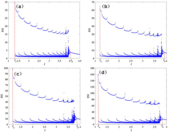
Figure 2.
ISI bifurcation diagram under I variation of different fractional-order q: (a) q = 0.6, (b) q = 0.7, (c) q = 0.8, (d) q = 0.9.
Case 1: when q = 0.6, then = 1.31, = 4.04, and , as shown in Figure 2a;
Case 2: when q = 0.7, then = 1.2, = 3.91, and , as shown in Figure 2b;
Case 3: when q = 0.8, then = 1.16, = 3.86, and , as shown in Figure 2c;
Case 4: when q = 0.9, then = 1.13, = 3.82, and , as shown in Figure 2d.
It can be seen from the above data that as the fractional order decreases, increases, indicating that the cluster firing or two-cycle firing may be larger under a fractional order.
In a word, the effect of fractional-order q on the firing of HR neurons is very obvious, and the range of external stimulation parameters can be wider by fractional-order q, which is more in line with the actual firing characteristics of neurons.
3. Firing Characteristic Analysis
3.1. Calculation of Lyapunov Exponent of Fractional-Order System
The Lyapunov exponent is an important method to describe the dynamics of a chaotic system, and it is also one of the quantitative indexes to judge whether it is a chaotic system. The Lyapunov exponent method for integer-order nonlinear systems is mature, and there is a Matlab2022b software toolkit to calculate it. However, there is no unified algorithm for the Lyapunov exponent of fractional-order chaotic systems. Most scientists use the time series of fractional chaotic systems to solve it, and less consideration is given to the equation. According to the Adomian decomposition method, this paper rewrites the fractional nonlinear system as follows:
The Jacobian matrix of iterative Equation (22) is given by as follows:
Through Equation (21), we can see that the more items there are in the Adomian decomposition algorithm, the more complex the Jacobian matrix of the equation is. For the convenience of calculation, we use the Jacobian () function in Matlab2022b software to obtain it and calculate it according to the QR decomposition definition. The process is as follows [34]:
Finally, the Lyapunov exponent is obtained by [34]
where k is the dimension of the system, ; h is the iteration time step.
3.2. Firing Characteristic Analysis
In order to study the firing phenomenon of fractional HR neurons under the electric field of DC stimulation, this paper uses Matlab software to simulate and quantitatively analyze the generated membrane potential curve, phase diagram, bifurcation diagram of the interspike interval (ISI) [9], and largest Lyapunov exponent (LLE) with external stimulation as variables.
In order to study the influence of the external stimulus DC on the firing characteristics of neurons, the external stimulus power I is selected as a variable, and its variation range is . Other parameters are fixed values: a = 1.0, b = 3.0, c = 1.0, d = 5.0, s = 4.0, r = 0.006, = −1.61. Select fractional-order q = 0.95; the bifurcation diagram of its neuron model is shown in Figure 3, and the maximum Lyapunov exponent is shown in Figure 2.
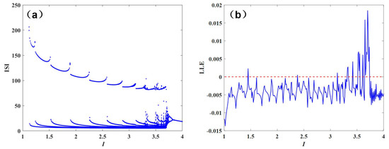
Figure 3.
ISI bifurcation diagram and LLE of the system when I changes: (a) Interspike interval (ISI) bifurcation diagram and (b) LLE.
From the bifurcation diagram, we can see that there are many chaotic regions represented by q = 0.95, and this explosive discharge activity is extremely likely to occur. At the same time, when I is from 3.2 to 3.7, the periodic burst firing and chaos burst firing appear alternately in the model, and the LLE of the chaotic system is greater than 0.
When , it can be seen from the bifurcation diagram that the system is not in the firing state, and we have drawn the phase diagram and time series of neurons at this time as shown in Figure 4. It can be seen that the system is at rest at this time, and the brain is resting or sleeping at this time.
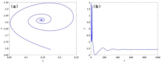
Figure 4.
Phase diagram and time series of neuron firing when I = 1: (a) phase diagram and (b) time series.
Figure 5a,b show the neurodynamic behavior when . It can be seen from Figure 5a that neurons show a periodic bursting pattern. Its bursting period is about 144 s, and there are about 5 spikes in a bursting period. The dependence of this number on I needs further study. In another bursting period, the interspike interval changes one after another, ranging from about 6 to 14 time units. From the point of view of nonlinear dynamics, the behavior of neurons is a kind of multiperiod oscillation behavior. The phase diagram in Figure 5a shows this multiperiod behavior more clearly, and it is a kind of burst firing behavior.
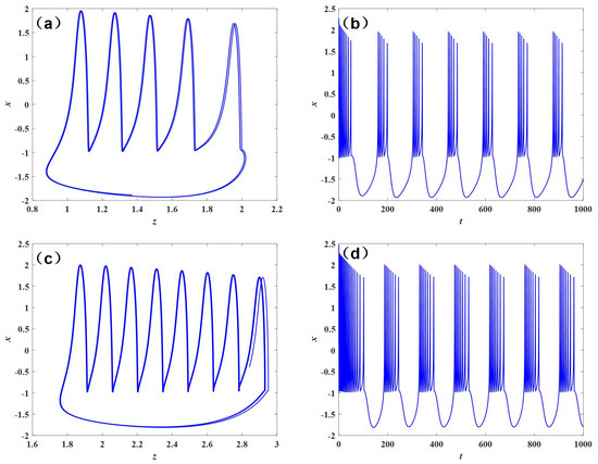
Figure 5.
Chaotic attractor and firing time series of model (1) with , I = 2 or I = 3: (a) chaotic attractor when I = 2; (b) firing time series I = 2; (c) chaotic attractor when I = 3; (d) firing time series I = 3.
Figure 5c,d show the neurodynamic behavior when . It can be seen from Figure 5c that neurons show a periodic bursting pattern. Its bursting period is about 143 s, and there are about 8 spikes in a bursting period. In another bursting period, the interspike interval changes one after another, ranging from about 6 to 15 time units. From the point of view of nonlinear dynamics, the behavior of neurons is a kind of multiperiod oscillation behavior. The phase diagram in Figure 5c shows this multiperiod behavior more clearly, and it is a kind of burst firing behavior.
Figure 6a,b show the neurodynamic behavior when . It can be seen from Figure 6a that neurons show a periodic bursting pattern. Its bursting period is about 120 s, and there are about 4 spikes in a bursting period. The dependence of this number on I needs further study. In another bursting period, the interspike interval changes one after another, ranging from about 5 to 14 time units. From the point of view of nonlinear dynamics, the behavior of neurons is a kind of multiperiod oscillation behavior. The phase diagram in Figure 6a shows this multiperiod behavior more clearly, and it is a kind of burst firing behavior.
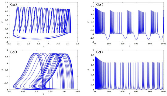
Figure 6.
Chaotic attractor and firing time series of model (1) with , I = 3.53 or I = 3.72: (a) chaotic attractor when I = 3.53; (b) firing time series I = 3.53; (c) chaotic attractor when I = 3.72; (d) firing time series I = 3.72.
Figure 6c,d show the neurodynamic behavior when . It can be seen from Figure 6c that neurons show a chaos bursting pattern.
Figure 7a,b show the neurodynamic behavior when . It can be seen from Figure 7a that neurons show a periodic spiking pattern. Its spiking period is 2. At this time, the neuron state is double-period.
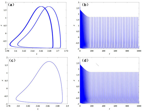
Figure 7.
Chaotic attractor and firing time series of model (1) with , I = 3.8 or I = 4: (a) chaotic attractor when I = 3.8; (b) firing time series I = 3.8; (c) chaotic attractor when I = 4; (d) firing time series I = 4.
4. Design of Sliding Mode Controller
4.1. Full Controller
With system (11) as the driving system, the response system is designed as follows on the third row:
The definition error , which is obtained by subtracting the above two formulas.
Lemma 1.
Assuming that = 0 is the equilibrium point of the fractional-order system an area containing the origin, if Lyapunov function is a continuous derivable function, and the local Lipschitz condition is satisfied with respect to x, the following conditions hold:
- (1)
- (2)
- ;
- (3)
- ;
where , and β are arbitrary normal numbers. Then the system is stable for a finite time, and the stable time of the system satisfies .
Theorem 1.
Design sliding surface , the input is
System (10) is synchronized with sliding mode (26) in finite time, where .
Proof.
on the sliding surface, so . Substituting the controller into the second equation of Equation (28) gives , so .
Substituting the controller into the third equation of Equation (11) gives , so .
When not on the sliding surface, design , and find the fractional derivative:
Therefore, , according to lemma 1, is obtained after simplification. □
4.2. Under Controller
With system (10) as the driving system, the response system is designed as follows:
The definition error , which is obtained by subtracting the above two formulas.
Theorem 2.
The design slip surface is . The controller is ; then system (10) is synchronized with sliding mode (21) in finite time, where .
Proof.
on the sliding surface, so . On the other hand, is obtained according to the third equation of formula (13), so .
According to ,, the trajectory of the chaotic system is bounded, and , so the second equation of Equation (13) becomes , .
When not on the sliding surface, design , and find the fractional derivative:
Therefore, , according to lemma 1, is obtained after simplification. □
4.3. Controller Simulation Results
In order to better verify the effectiveness of the controller, we generally use the timing state of the drive system and the response system and the error diagram of the timing state to describe it.
When a = 1.0, b = 3.0, c = 1.0, d = 5.0, s = 4.0, r = 0.006, = −1.61, = 0.1, = 0.2, = 0.3, and I = 3.53, the system is in a chaotic state, and the initial values are [0.1,0.2,0.1,0.4] and [4,2,5,4] without the controller; the time series and error diagram of two fractional-order neuron models are shown in Figure 8. As can be seen from Figure 8, the initial values of the response system are different, and the states are particularly different without a controller, which means that the system is lazy to the initial values, which is in line with the chaotic nature, and also shows that the neuron model is chaotic under this parameter.
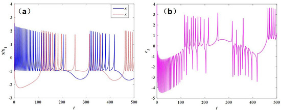
Figure 8.
System time series and error diagram without controller: (a) time series and (b) system error diagram.
Initial values are [0.1,0.2,0.1,0.4] and [4,2,5,4]. The full controller is simulated by Matlab, and the synchronization results and error results are shown in Figure 9a,b. The under controller is simulated by Matlab, and the synchronization results and error results are shown in Figure 9c,d. As can be seen from the figure, both controllers can achieve the same effect, and the simulation results show its realizability and the effectiveness of the controller. The full controller can achieve control within 5 s, the under controller can achieve control within 3 s, and the under controller is superior to the full controller in time rapidity. In addition, the effect of the under controller is better (faster) than that of the full controller, which shows that for complex systems, control can be realized by simple controllers in a short time, and these controllers can be realized by external circuits of neurons and act as external stimulus currents.
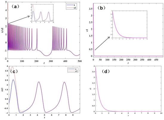
Figure 9.
System variable synchronization state diagram and error diagram: (a) synchronization state diagram with full controller, (b) system error diagram with full controller, (c) synchronization state diagram with under controller, (d) system error diagram with under controller.
5. Conclusions
In this work, the fractional-order HR neuron system is numerically solved by the Adomian decomposition method, the phase diagram and ISI bifurcation diagram of the neuron model are drawn, various firing behaviors of the system are analyzed, and the influence of fractional order on the system firing is also expounded. At the same time, the dynamic behavior of the system is analyzed by using the LLE and complexity. Through the above analysis, it is concluded that the fractional order affects the range of external stimulus current, and the lower the fractional order, the larger the range of external stimulus current corresponding to chaos and burst firing. In addition, the sliding mode control algorithm is used to design the full controller and the under controller of the system, and Matlab is used to simulate the controller. The simulation results illustrate the realizability of the controller, and it is found that the short time response of the controller is better, and the research results provide theoretical support for the coding of neurons and information transmission.
On the basis of the research, we can study the dynamics and firing behavior of the neural network formed by the coupling of multiple fractional-order neurons, and also study the influence of the firing behavior of each neuron. Of course, the research method of fractional calculus adopted in this paper can also be applied to the engineering field [35,36,37].
Author Contributions
Conceptualization, T.L.; methodology, T.L. and H.F.; software, H.F. and H.Z.; validation, T.L. and H.Z.; formal analysis, T.L.; investigation, H.F.; resources, T.L.; data curation, T.L.; writing—original draft preparation, H.F.; writing—review and editing, T.L., H.Z. and L.H.; visualization, T.L. and H.F.; supervision, W.S.; project administration, T.L. All authors have read and agreed to the published version of the manuscript.
Funding
This work was supported by the Shandong Provincial Natural Science Foundation (ZR2022MA073), Shandong Province Science and Technology Small and Medium-Sized Enterprises Innovation Ability Promotion Project (Grant No. 2021TSGC1467), Key Research and Development Plan of Shandong Province (2019GGX104092), Natural Science Foundation of Shandong Province (ZR2017PA008), and Science and Technology Plan Projects of Universities of Shandong Province (J18KA381).
Institutional Review Board Statement
Not applicable.
Informed Consent Statement
Not applicable.
Data Availability Statement
All datasets generated for this study are included in the article.
Conflicts of Interest
The authors declare no conflict of interest.
References
- Tsumoto, K.; Kitajima, H.; Yoshinaga, T.; Aihara, K.; Kawakami, H. Bifurcations in Morris-Lecar neuron model. Neurocomputing 2006, 69, 293–316. [Google Scholar]
- Ma, K.J.; Tang, J. A review for dynamics in neuron and neuronal network. Nonlinear Dyn. 2017, 89, 1569–1578. [Google Scholar]
- Qishao, L. Neurodynamics and Mechanics. J. Dyn. Control. 2020, 18, 6–10. [Google Scholar]
- Lapicque, L. Recherches quantitatives sur 1’excitation electrique des nerfs traitescomme une polarization. J. Physiol. 1907, 9, 622. [Google Scholar]
- Hodgkin, A.L.; Huxley, A.F. A quantitative description of membrane current andits application to conduction and excitation in nerve. Physiology 1952, 117, 500–544. [Google Scholar]
- Nagumo, J.; Arimoto, S.; Yoshizawa, S. An Active Pulse Transmission LineSimulating Nerve Axon. Proc. IRE 1962, 50, 2061–2070. [Google Scholar]
- Fitzhugh, R. Impulses and physiological states in theoretical models of nervemembrane. Biophys. J. 1961, 1, 445–466. [Google Scholar] [CrossRef]
- Hindmarsh, J.L.; Rose, R.M. A model of the nerve impulse using two first-orderdifferential equations. Nature 1982, 296, 162–164. [Google Scholar]
- Bao, H.; Hu, A.; Liu, W.; Bao, B. Hidden bursting firings and bifurcation mechanisms in memristive neuron model with threshold electromagnetic induction. IEEE Trans. Neural Netw. Learn. Syst. 2019, 31, 502–511. [Google Scholar]
- Lv, M.; Wang, C.; Ren, G.; Ma, J. Model of electrical activity in a neuron under magnetic flow effect. Nonlinear Dyn. 2016, 85, 1479–1490. [Google Scholar]
- Wu, F.; Wang, C.; Xu, Y.; Ma, J. Model of electrical activity in cardiac tissue under electromagnetic induction. Sci. Rep. 2016, 6, 68. [Google Scholar]
- Wang, Y.; Ma, J.; Xu, Y.; Wu, F.; Zhou, P. The Electrical Activity of Neurons Subject to Electromagnetic Induction and Gaussian White Noise. Int. J. Bifurc. Chaos 2017, 27, 1750030. [Google Scholar]
- Li, Z.J.; Xie, W.Q.; Zeng, J.F.; Zeng, Y.C. Firing activities in a fractional-order Hindmarsh-Rose neuron with multistable memristor as autapse. Chin. Phys. B 2022, 32, 010503. [Google Scholar]
- Shivam MalikMir, A.H. FPGA Realization of Fractional Order Hindmarsh Rose Neuron. Appl. Math. Model. 2019, 81, 372–385. [Google Scholar]
- Yu, Y.; Shi, M.; Kang, H.; Chen, M.; Bao, B. Hidden dynamics in a fractional-order memristive Hindmarsh— Rose model. Nonlinear Dyn. 2000, 100, 891–906. [Google Scholar]
- Fu, H.; Lei, T. Adomian Decomposition, Dynamic Analysis and Circuit Implementation of a 5D Fractional-Order Hyperchaotic System. Symmetry 2022, 14, 484. [Google Scholar] [CrossRef]
- Berkal, M.; Almatrafi, M.B. Bifurcation and Stability of Two-Dimensional Activator–Inhibitor Model with Fractional-Order Derivative. Fractal Fract. 2023, 7, 344. [Google Scholar] [CrossRef]
- Khan, A.Q.; Bukhari, S.A.H.; Almatrafi, M.B. Global dynamics, Neimark-Sacker bifurcation and hybrid control in a Leslie’s prey-predator model. Alex. Eng. J. 2022, 61, 11391–11404. [Google Scholar]
- Meng, F.; Zeng, X.; Wang, Z.; Wang, X. Adaptive Synchronization of Fractional-Order Coupled Neurons Under Electromagnetic Radiation. Int. J. Bifurc. Chaos 2020, 30, 2050044. [Google Scholar]
- Malik, S.A.; Mir, A.H. Synchronization of Fractional Order Neurons in Presence of Noise. IEEE/ACM Trans. Comput. Biol. Bioinform. 2020, 19, 1887–1896. [Google Scholar]
- Wang, S.; Wei, Z.; Wei, Z. Synchronization of coupled memristive Hindmarsh-Rose maps under different coupling conditions. Int. J. Electron. Commun. 2023, 161, 154561. [Google Scholar]
- Rehák, B.; Lynnyk, V. Synchronization of a Network Composed of Stochastic Hindmarsh–Rose Neurons. Mathematics 2021, 9, 2625. [Google Scholar] [CrossRef]
- Ding, K.; Han, Q.L. Master–slave synchronization criteria for chaotic Hindmarsh–Rose neurons using linear feedback control. Complexity 2016, 21, 319–327. [Google Scholar]
- Nguyen, L.H.; Hong, K.S. Adaptive synchronization of two coupled chaotic Hindmarsh–Rose neurons by controlling the membrane potential of a slave neuron. Appl. Math. Model. 2013, 37, 2460–2468. [Google Scholar]
- Ding, K.; Han, Q.L. Synchronization of two coupled Hindmarsh–Rose neurons. Kybernetika 2015, 51, 784–799. [Google Scholar]
- Hettiarachchi, I.T.; Lakshmanan, S.; Bhatti, A.; Lim, C.P.; Prakash, M.; Balasubramaniam, P.; Nahavandi, S. Chaotic synchronization of time-delay coupled Hindmarsh–Rose neurons via nonlinear control. Nonlinear Dyn. 2016, 86, 1249–1262. [Google Scholar]
- Equihua, G.G.V.; Ramirez, J.P. Synchronization of Hindmarsh–Rose neurons via Huygens-like coupling. IFAC-PapersOnLine 2018, 51, 186–191. [Google Scholar]
- Yu, H.; Peng, J. Chaotic synchronization and control in nonlinear-coupled Hindmarsh–Rose neural systems. Chaos Solitons Fractals 2006, 29, 342–348. [Google Scholar]
- Xu, Y.; Jia, Y.; Ma, J.; Alsaedi, A.; Ahmad, B. Synchronization between neurons coupled by memristor. Chaos Solitons Fractals 2017, 104, 435–442. [Google Scholar]
- Bandyopadhyay, A.; Kar, S. Impact of network structure on synchronization of Hindmarsh–Rose neurons coupled in structured network. Appl. Math. Comput. 2018, 333, 194–212. [Google Scholar]
- Li, C.; Su, K.; Tong, Y.; Li, H. Robust synchronization for a class of fractional-order chaotic and hyperchaotic systems. Opt.-Int. J. Light Electron Opt. 2013, 124, 3242–3245. [Google Scholar] [CrossRef]
- Cherruault, Y.; Adomian, G. Decomposition methods: A new proof of convergence. Math. Comput. Model. 1993, 18, 103–106. [Google Scholar] [CrossRef]
- Hindmarsh, J.L.; Rose, R.M. A model of neuronal bursting using three coupled first order differential equations. Proc. R. Soc. Lond. Biol. Sci. 1984, 221, 87–102. [Google Scholar]
- Bremen, H.F.V.; Udwadia, F.E.; Proskurowski, W. An efficient QR based method for the computation of Lyapunov exponents. Physica D 1997, 101, 1–16. [Google Scholar] [CrossRef]
- Yasmin, H.; Aljahdaly, N.H.; Saeed, A.M.; Shah, R. Investigating Families of Soliton Solutions for the Complex Structured Coupled Fractional Biswas–Arshed Model in Birefringent Fibers Using a Novel Analytical Technique. Fractal Fract. 2023, 7, 491. [Google Scholar] [CrossRef]
- Yasmin, H.; Aljahdaly, N.H.; Saeed, A.M.; Shah, R. Probing Families of Optical Soliton Solutions in Fractional Perturbed Radhakrishnan–Kundu–Lakshmanan Model with Improved Versions of Extended Direct Algebraic Method. Fractal Fract. 2023, 7, 512. [Google Scholar] [CrossRef]
- Zhang, K.; Alshehry, A.S.; Aljahdaly, N.H.; Shah, N.A.; Ali, M.R. Efficient computational approaches for fractional-order Degasperis-Procesi and Camassa-Holm equations. Results Phys. 2023, 50, 106549. [Google Scholar] [CrossRef]
Disclaimer/Publisher’s Note: The statements, opinions and data contained in all publications are solely those of the individual author(s) and contributor(s) and not of MDPI and/or the editor(s). MDPI and/or the editor(s) disclaim responsibility for any injury to people or property resulting from any ideas, methods, instructions or products referred to in the content. |
© 2023 by the authors. Licensee MDPI, Basel, Switzerland. This article is an open access article distributed under the terms and conditions of the Creative Commons Attribution (CC BY) license (https://creativecommons.org/licenses/by/4.0/).