Article

Ultra-Short-Term Load Forecasting for Customer-Level Integrated Energy Systems Based on Composite VTDS Models

School of Electrical and Electronic Engineering, North China Electric Power University, Baoding 071003, China
*
Author to whom correspondence should be addressed.
Processes 2023, 11(8), 2461; https://doi.org/10.3390/pr11082461
Submission received: 3 July 2023 / Revised: 4 August 2023 / Accepted: 14 August 2023 / Published: 16 August 2023

Abstract

:
A method is proposed to address the challenging issue of load prediction in user-level integrated energy systems (IESs) using a composite VTDS model. Firstly, an IES multi-dimensional load time series is decomposed into multiple intrinsic mode functions (IMFs) using variational mode decomposition (VMD). Then, each IMF, along with other influential features, is subjected to data dimensionality reduction and clustering denoising using t-distributed stochastic neighbor embedding (t-SNE) and fast density-based spatial clustering of applications with noise (FDBSCAN) to perform major feature selection. Subsequently, the reduced and denoised data are reconstructed, and a time-aware long short-term memory (T-LSTM) artificial neural network is employed to fill in missing data by incorporating time interval information. Finally, the selected multi-factor load time series is used as input into a support vector regression (SVR) model optimized using the quantum particle swarm optimization (QPSO) algorithm for load prediction. Using measured load data from a specific user-level IES at the Tempe campus of Arizona State University, USA, as a case study, a comparative analysis between the VTDS method and other approaches is conducted. The results demonstrate that the method proposed in this study achieved higher accuracy in short-term forecasting of the IES’s multiple loads.

1. Introduction

With the development of climate change and the increasing awareness of environmental issues, the current energy transition is focused on low-carbon and sustainable development [1,2]. In recent years, integrated energy systems (IESs) have experienced rapid growth and have been widely studied and implemented in various countries. However, the strong randomness, volatility, and coupling of multiple loads in IES operations can have an impact on its economic and reliable operation, particularly the frequent fluctuations of user-level IES multiple loads. Therefore, the accurate prediction of user-level IES multiple loads is essential for the stable operation of the system.
Over the past few decades, various load forecasting methods have been proposed for the integrated energy system (IES), including regression analysis [3], correlation analysis [4], and time series analysis [5]. However, these statistical methods have limitations in terms of their ability to handle nonlinear data and achieve high prediction accuracy. To address these limitations, researchers have turned to artificial intelligence methods, such as artificial neural networks (ANNs) [6], decision trees, and support vector machines (SVMs) [7]. Among these, ANN stands out for its strong decision-making capabilities under uncertain conditions. In recent years, the application of deep learning has become increasingly prevalent, and researchers have combined convolutional neural networks (CNNs) with various decomposition algorithms to adapt network structures and parameters for load forecasting studies.
In the literature [8], four baseline models, including ANN, SVM, classification and regression trees (CARTs), and long short-term memory (LSTM), with a standard architecture were used to predict hourly residential load demand in the IES. However, these models were only suitable for specific scenario predictions and lacked generalization performance verification. In the literature [9], an attention-based CNN-LSTM [10] model was proposed for short-term load forecasting in IES. Although the model considered factors such as hourly electricity prices and household energy efficiency, it failed to capture dynamic changing characteristics, resulting in low prediction accuracy.
The literature [11] presented an IES load forecasting model based on bidirectional generative adversarial network (BiGAN) data augmentation and transfer learning. However, the model did not consider factors such as user variations, and the dataset for new users was limited, lacking sufficient data support. In the literature [12,13], a hybrid load forecasting model integrating intelligent methods was proposed for feature selection and parameter optimization. However, this method suffered from negative transfer effects. In the literature [14], a cross-location IES load forecasting method that considered time and multi-location data was introduced, avoiding negative transfer effects. However, the subjective setting of model parameters in this approach led to decreased prediction accuracy. The aforementioned models focused on deterministic load forecasting for IES multiple loads and made improvements mainly in terms of multi-model fusion algorithms. Although they considered multi-dimensional features of the data, they had shortcomings in data cleaning, such as outlier detection and missing value imputation, as well as significant feature selection, which affected prediction accuracy.
To address this issue, this study investigates a load forecasting model based on the composite VTDS model. Firstly, the IES multivariate load time series is decomposed into multiple intrinsic mode functions (IMFs) using variational mode decomposition (VMD). Subsequently, the multivariate load time series, consisting of the IMFs and other influencing features, undergoes t-distributed stochastic neighbor embedding (t-SNE) for dimensionality reduction and fast density-based spatial clustering of applications with noise (FDBSCAN) for noise reduction, enabling the selection of major features in the multivariate load time series. The sequence data are then restored and missing values are filled using a time-aware long short-term memory (T-LSTM) artificial neural network, thereby completing the data cleaning and feature selection steps. Finally, the feature-selected multivariate load time series is input into the support vector regression (SVR) model for prediction. The SVR model is optimized using the quantum particle swarm optimization (QPSO) algorithm. The effectiveness of the proposed composite fusion model prediction method is validated through case studies.

2. Variational Mode Decomposition

To enhance load prediction accuracy and prevent overfitting, the VMD decomposition method [15] is employed to decompose the multiple-load time series data of IES. VMD effectively breaks down the time series data into several IMFs with physical significance. This decomposition is achieved by transforming the signal decomposition process into an iterative variational problem, ensuring robustness against noise interference. The decomposition process can be summarized as follows.
The eigenmode functions, u k ( t ) = A k ( t ) cos ( ϕ k ( t ) ) , of the IES multivariate load series, f ( t ) , are subjected to Hilbert transformations, as shown in Equation (1):
u k 1 ( t ) = δ ( t ) + j π t u k ( t )
where δ ( t ) is the impulsive function and obeys Dirac distribution.
Using exponential, e j ω k t , correction for the modal functions, u k 1 ( t ) , the spectrum of each modal function is modulated to the whole frequency band using Equation (2):
u k 2 ( t ) = δ ( t ) + j π t u k ( t ) e j ω k t
where ω k is the center frequency of u k 2 ( t ) .
Using Gaussian smoothing to demodulate each modal signal, the bandwidth is obtained, as shown in Equation (3):
b = t δ ( t ) + j π t u k ( t ) e j ω k t 2 2
The essence of the variational problem is to decompose the original signal, x ( t ) , into K components, u ( t ) , then demodulate it using Hilbert transform to obtain the envelope signal, and, finally, mix it with the predicted center frequency, ω k . The constraints are constructed, as shown in Equation (4):
min { u k } , { ω k } k = 1 K t δ ( t ) + j π t * u k ( t ) e j ω k t 2 2 s . t . k = 1 K u k ( t ) = f ( t )
where u k = { u 1 , u 2 , u k } is each modal function; ω k = ω 1 , ω 2 , , ω k is each modal center frequency. Using the quadratic equilibrium parameters, α , and Lagrange multipliers, λ ( t ) , the unconstrained variational problem is constructed, as shown in Equation (5):
L u k , ω k , λ = α k = 1 K t δ ( t ) + j π t u k ( t ) e j ω k t 2 2 + f ( t ) k = 1 K u k ( t ) 2 2 + λ ( t ) , f ( t ) k = 1 K u k ( t )
where ω 0 , the alternating direction method of multipliers (ADMMs), is used for the convex optimization solution; the generalized functions, u k and ω k , are updated, as shown in Equation (6):
u ^ k n + 1 ( ω ) = f ( ω ) i = 1 ,   i < k K u ^ k n + 1 ( ω ) i = 1 ,   i > k K u ^ k n ( ω ) + λ ^ n ( ω ) 2 1 + 2 α ( ω ω k n ) 2 ω k n + 1 = 0 ω u ^ k n + 1 ( ω ) 2 d ω 0 u ^ k n + 1 ( ω ) 2 d ω
where n is the number of iterations; u ^ k n + 1 ( ω ) , f ^ ( ω ) , and λ ^ n ( ω ) are the Fourier transforms of u ^ k n + 1 ( t ) , f ( t ) , and λ ( t ) , respectively, for all ω 0 ; and λ is updated, as shown in Equation (7):
λ ^ n + 1 ( ω ) = λ ^ n ( ω ) + τ f ^ ( ω ) k u ^ k n + 1 ( ω )
where τ is the noise tolerance; when there is strong noise in the signal, it is necessary to set τ = 0 to achieve a better prediction effect set, iterate until the convergence condition of Equation (8) is satisfied, and, finally, obtain IMFs:
k = 1 K u ^ k n + 1 u ^ k n 2 2 / u ^ k n 2 2 < ε
where ε is the tolerance error.

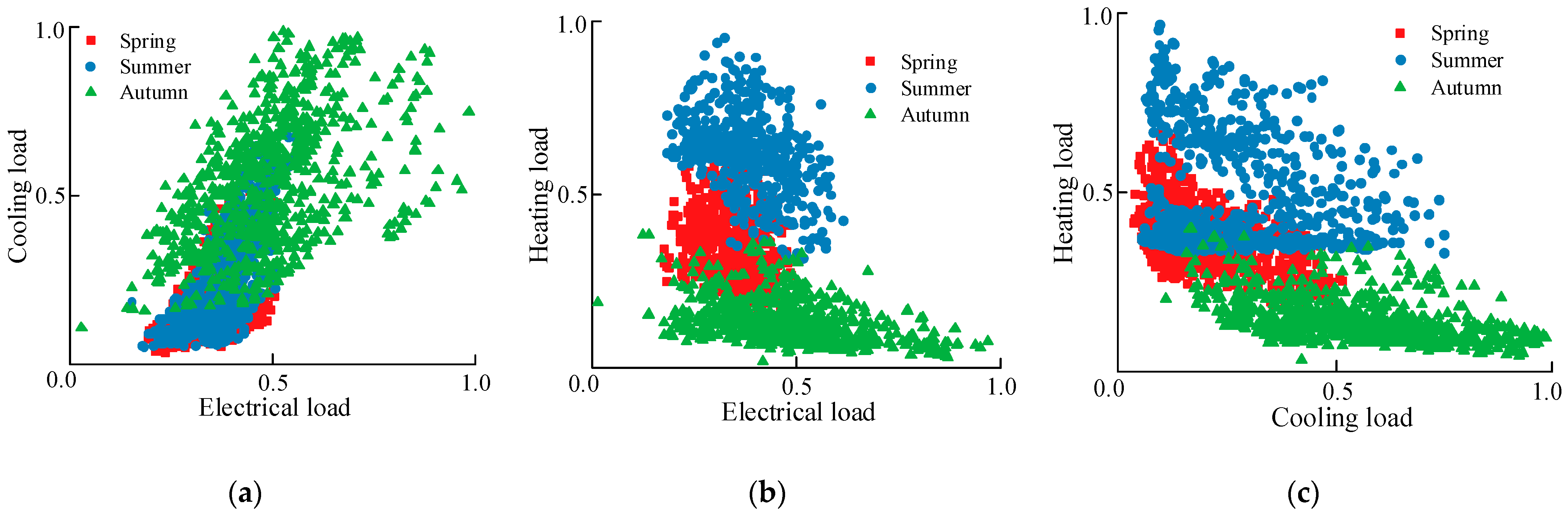
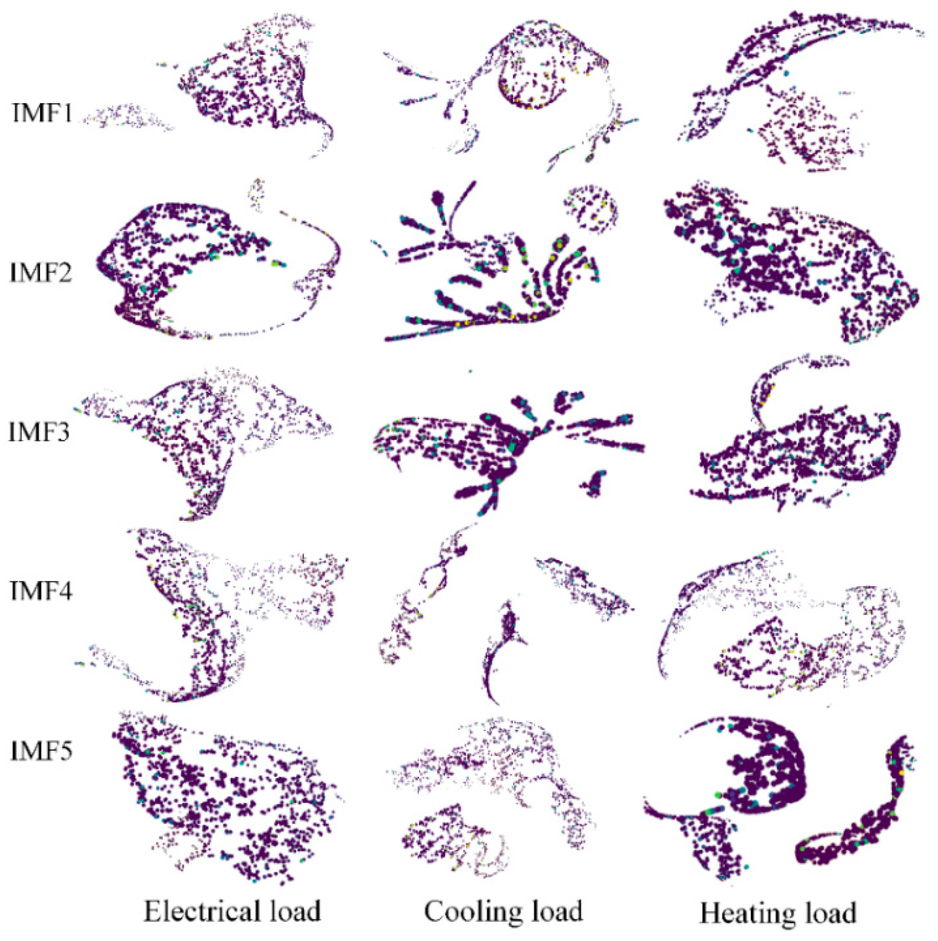
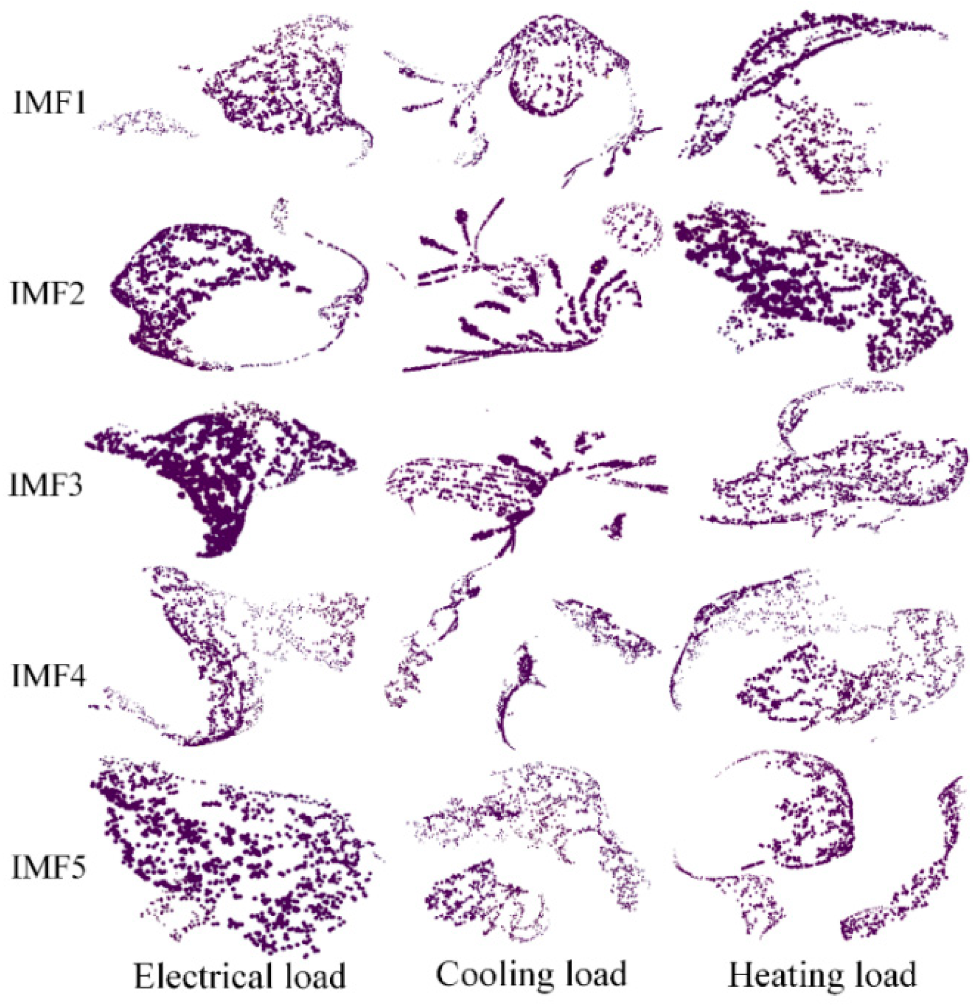
3. t-SNE Data Dimensionality Reduction and FDBSCAN Clustering Noise Reduction

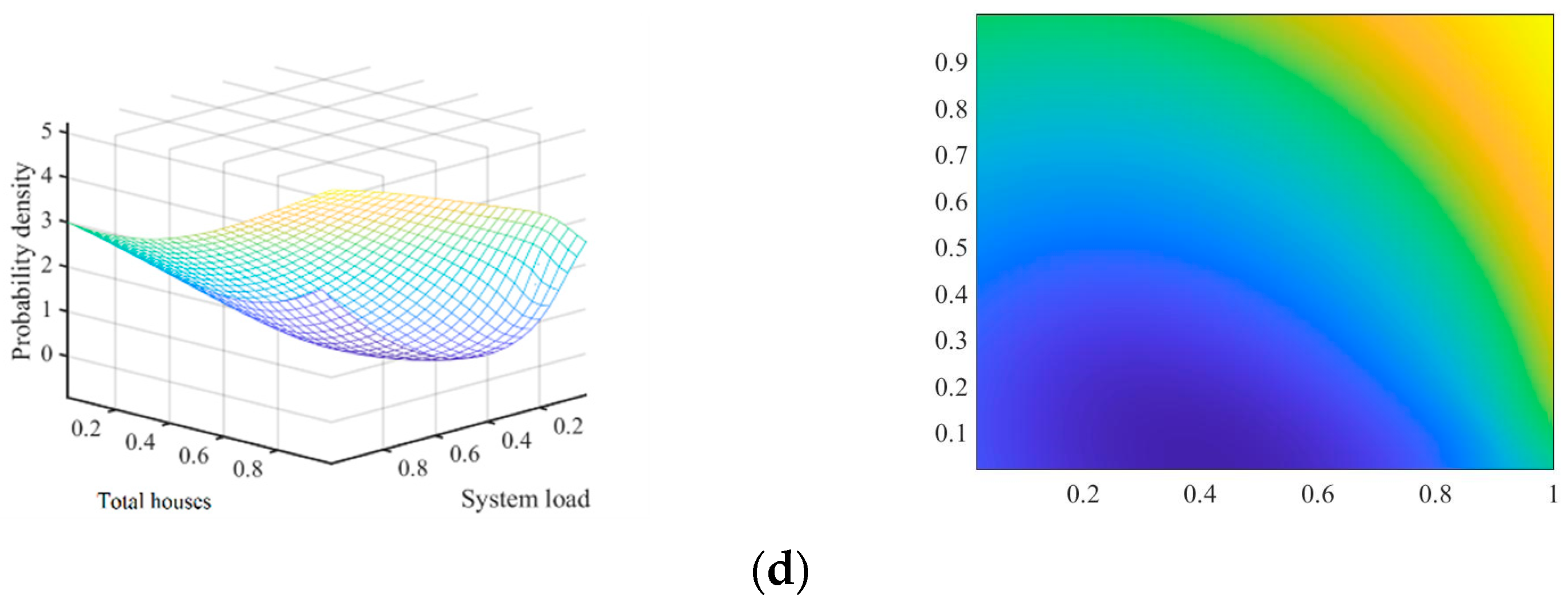
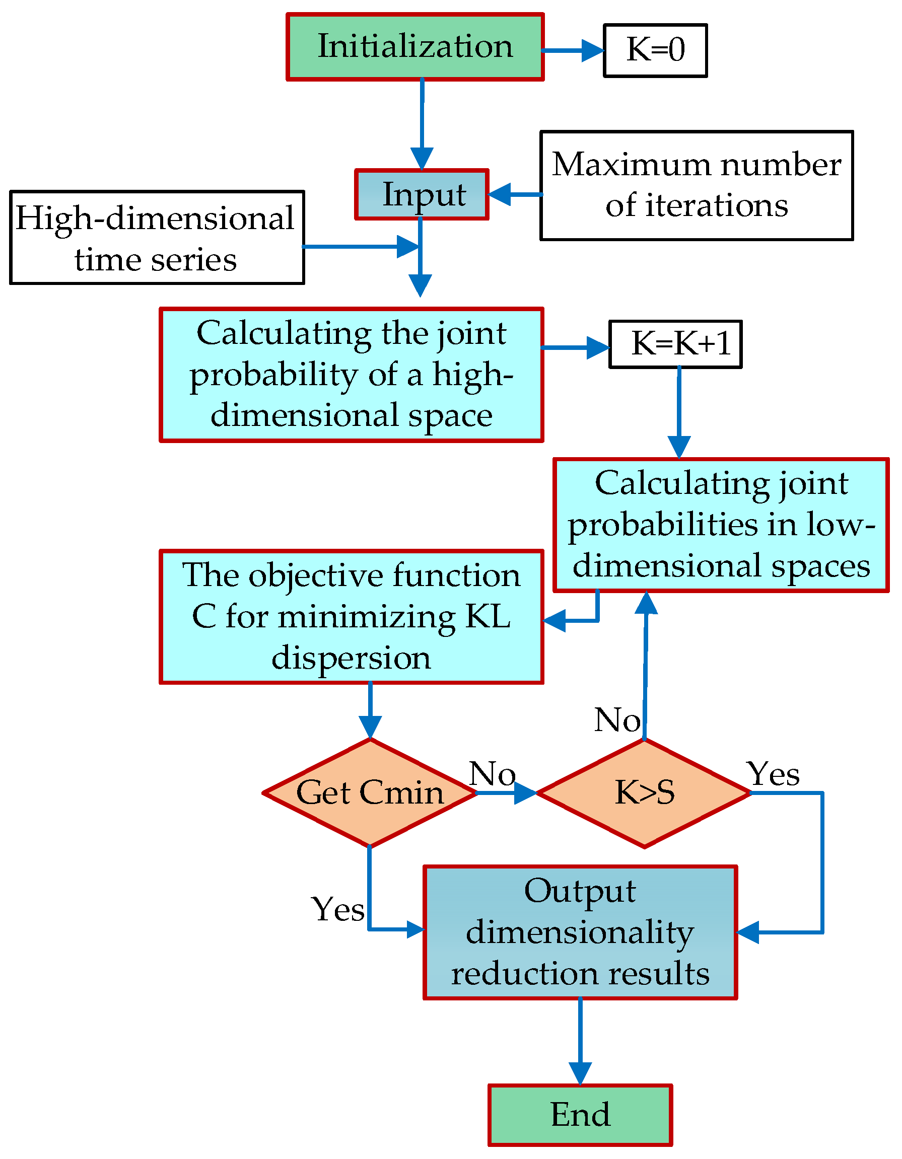
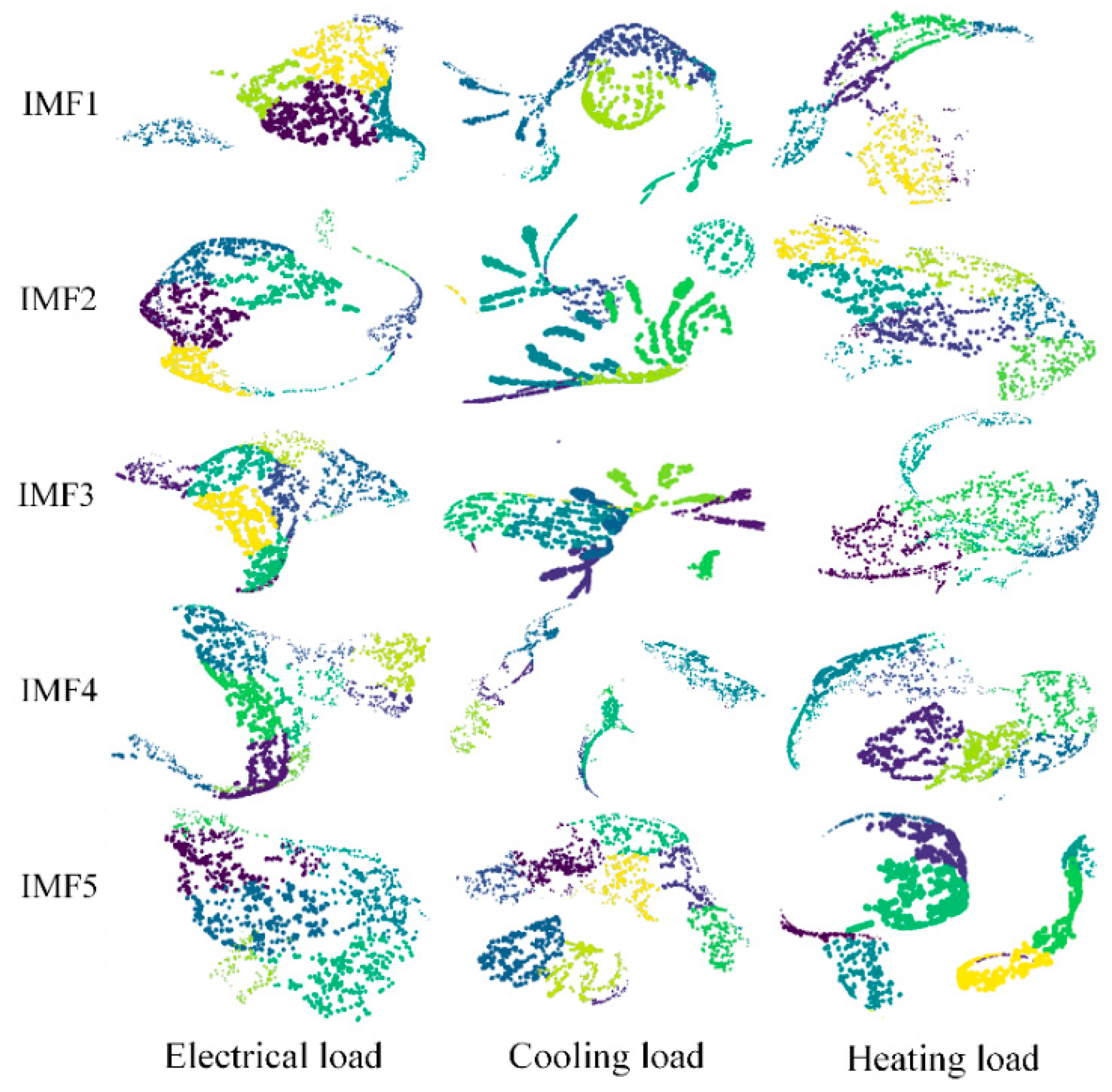
3.1. Data Compression and Dimensionality Reduction Based on the t-SNE Algorithm

This paper presents seasonal plots of the hourly cooling load distribution, cooling and heating load distribution, and electric heat load distribution for the Tempe campus of Arizona State University in the United States. The data cover the period from January to June 2022 and are generated using a sparse method. These plots are depicted in Figure 1. Furthermore, a Pearson correlation matrix is provided, showcasing the relationships between the multivariate system load and variables such as temperature, carbon emissions, the total number of lighting fixtures, and the number of residential buildings. The probability density distribution of the correlation matrix is illustrated in Figure 1 and Table 1.
The correlations in Figure 1 are reflected in the fact that the demand variations of multiple loads in IES are not completely independent; a sudden change in one load can potentially serve as a signal transmitted to other loads. Figure 1 reveals two fundamental characteristics of load correlations in IES: in any time interval (season), different types of loads exhibit a certain degree of correlation; the two types of loads exhibit similar correlations in different time intervals, but the degree of correlation may vary. A Pearson correlation matrix for correlation analysis of system multivariate load and influencing factor is shown in Table 1.
Figure 2 provides an intuitive analysis of the correlation between variables and system load. The 3D plot and its pseudo-colored representation depict the complex correlation strength between total lightbulbs, temperature, greenhouse gases, total houses, and system load. The varying shades of different colors reflect the varying degrees of correlation. Deeper colors indicate stronger correlations, suggesting that when conducting load forecasting, these variables should be considered as influencing factors.
To determine the statistical significance of the correlation coefficients, a significance level of 0.05 was set. Then, the p-value for each correlation coefficient was calculated (i.e., the probability of the hypothesis test). If a p-value is less than 0.05, it can be considered that the correlation coefficient is statistically significant, indicating a significant correlation between the two variables. Through the above steps, the main influencing factors for load forecasting were selected. The main influencing factors consist of 14 types, namely, temperature, humidity, wind speed, sunshine hours, precipitation, holidays, seasons, total lightbulbs, greenhouse gas emissions, total houses, system load, population, and transmission line capacity. Based on the calculations from Table 1 and Figure 1 and Figure 2, it can be concluded that the strong interdependencies among multiple loads, temperature, carbon emissions, and other factors significantly impact the load forecast in the IES. Therefore, it is crucial to perform primary feature selection and dimensionality reduction on these influencing factors. To address the issue of crowded visualizations resulting from principal component analysis (PCA) algorithm-based dimensionality reduction [16], this paper adopts a two-step approach. Firstly, PCA is utilized to determine the order of dimensionality reduction. Subsequently, the t-SNE algorithm, a nonlinear learning method based on information theory, is introduced. t-SNE preserves the local characteristics of the data by transforming the proximity relationships into a probability distribution. The high-dimensional time series data, consisting of each IMF and other influencing factors obtained through VMD decomposition, is transformed into low-dimensional time series data using the gradient descent method. The iterative process continues until the difference loss function C reaches its minimum value, and the optimal dimensionality reduction result is obtained, satisfying the iteration condition. A flowchart of the algorithm is illustrated in Figure 3.
In Figure 3, K is used to indicate the number of nearest neighbors considered when constructing the neighborhood graph. S represents perplexity, which is used to balance the attention given to local structure and global structure in the data, while also controlling the effective number of neighbors used for each data point during the embedding process.

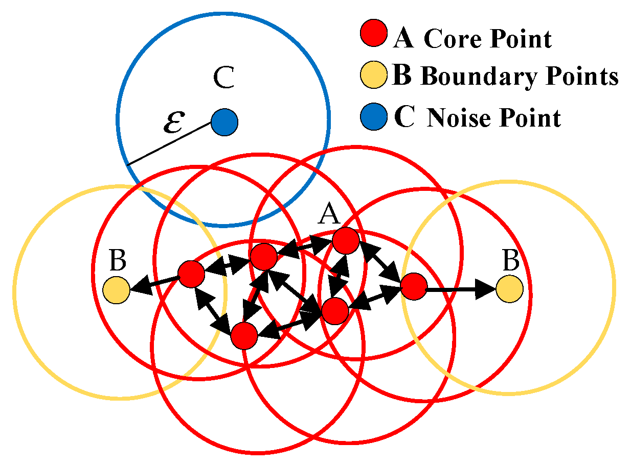
3.2. FDBSCAN Clustering Noise Reduction

The presence of noise and orphan points in the data, even after dimensionality reduction, can have a negative impact on load prediction accuracy. To mitigate this issue, DBSCAN is utilized. DBSCAN is an unsupervised machine learning method [17,18] that operates effectively in spatial databases containing noise. It divides regions with a sufficiently high density of connected points into clusters, allowing for the discovery of data structures of any shape without the need to specify the number of clusters in advance. Moreover, DBSCAN is capable of identifying and handling noise and outliers to reduce their impact. The DBSCAN algorithm relies on two crucial hyperparameters: the radius and the density threshold. These parameters play a significant role in determining the clustering behavior and noise identification. A schematic diagram illustrating the DBSCAN clustering process is presented in Figure 4.
The DBSCAN algorithm operates under the assumption that points within the neighborhood of the same core point belong to the same class. However, if the distance between two sets of sample points is larger than a certain threshold, this indicates that these points belong to different classes. This can result in redundant neighborhood retrieval during the cluster expansion process, which, in turn, slows down the clustering speed. To address this issue, this paper explores the Fast DBSCAN (FDBSCAN) algorithm. In the FDBSCAN algorithm, the core points existing in the overlapping region between sub-clusters are used as the basis for cluster merging. By utilizing these core points, extended cluster clustering is performed, effectively avoiding redundant neighborhood retrieval during cluster expansion. As a result, the clustering process is accelerated. A flowchart illustrating the FDBSCAN algorithm is depicted in Figure 5.

4. Data Restoration and Data Filling

After compressing the data, some or all of the redundancy may still remain during its utilization. Therefore, a restoration step is required to recover the original data. However, the restoration process may result in missing data. Consequently, the effectiveness of time series prediction is compromised. To address this issue, it is essential to not only consider the correlation between the data but also fill in the missing values. In this study, a novel unsupervised model called T-LSTM is proposed for filling in the missing data in time series. The T-LSTM model incorporates time interval information to enhance its predictive capabilities. The architecture of the T-LSTM model is depicted in Figure 6.
The T-LSTM model [19,20] leverages the interval time between data points as additional features. In Figure 6, the green box represents the network, and the yellow circles represent point-wise operators. x t represents the current input, h t 1 and h t are previous and current hidden states, and C t 1 and C t are previous and current cell memories. In the T-LSTM model, the interval information is carefully analyzed, weighted, fused, and incorporated into the LSTM network for training. By considering the interval information, the model is capable of accurately predicting and filling in the missing data. The LSTM network processes the input features and generates the output values that effectively fill the missing data points.

5. QPSO-Optimized SVR Model

5.1. SVR Model

The SVR model [21,22] is known for its strong generalization ability when dealing with high-dimensional nonlinear problems with limited data. It has been widely employed in various applications such as transmission line discharge, battery life prediction, and load prediction. The SVR model utilizes a kernel function to map the input data from a low-dimensional space to a higher-dimensional space. This transformation allows for linearly indistinguishable data to become linearly separable in the transformed space. In the SVR model, the input feature vector is denoted as x i , the corresponding output vector as y i , and n represents the total number of samples. To ensure the effectiveness of the SVR model in practical applications, a nonlinear mapping function is defined, as shown in Equation (9):
f ( x ) = ω φ ( x ) + b
The mapping of the training set from a low-dimensional space to a high-dimensional space is denoted by φ ( x ) : R n R N . The weight vector representing the smoothness of the model is denoted by ω , and b is the bias parameter. According to the risk minimization criterion, Equation (9) can be expressed as the following minimization problem:
min R = C i = 1 n ( ξ i + ξ i ) + 1 2 ω T ω
s . t . y i ω T φ ( x i ) b ε + ξ i y i + ω T φ ( x i ) + b ε + ξ i ξ i , ξ i 0 , i = 1 , 2 , , n
C represents the penalty factor for the slack variable. It accounts for the allowable error in the regression. The minimization problem is converted into a quadratic convex optimization problem through the introduction of Lagrange multipliers μ , μ , γ , γ 0 and optimality conditions.
L ( ω , b , ξ i , ξ i , μ , μ , γ , γ ) = 1 2 ω T ω + C i = 1 n ( ξ i + ξ i ) + i = 1 n μ i ( f ( x i ) y i ε ξ i ) + i = 1 n μ i ( f ( x i ) + y i ε ξ i ) i = 1 n ( ξ i γ i ξ i γ i )
By taking a partial derivative, ω , b , ξ i , ξ i , of the Lagrange function and maximizing its dual problem, the load prediction problem can be expressed by a kernel function, f ( x ) .
f ( x ) = i = 1 n ( μ μ ) κ ( x i , x j ) + b
In Equation (13), κ ( x i , x j ) = φ T ( x i ) φ ( x j ) is the kernel function that satisfies Mercer’s theorem. The kernel function avoids the direct calculation of arbitrary dimensional feature space mapping. In this paper, the radial basis function (RBF) kernel is used due to its fewer parameters and stronger nonlinear mapping capabilities. The expression of the RBF kernel is as shown in Equation (14):
κ ( x i , x j ) = exp ( υ x i x j 2 )
where υ is the nuclear parameter.

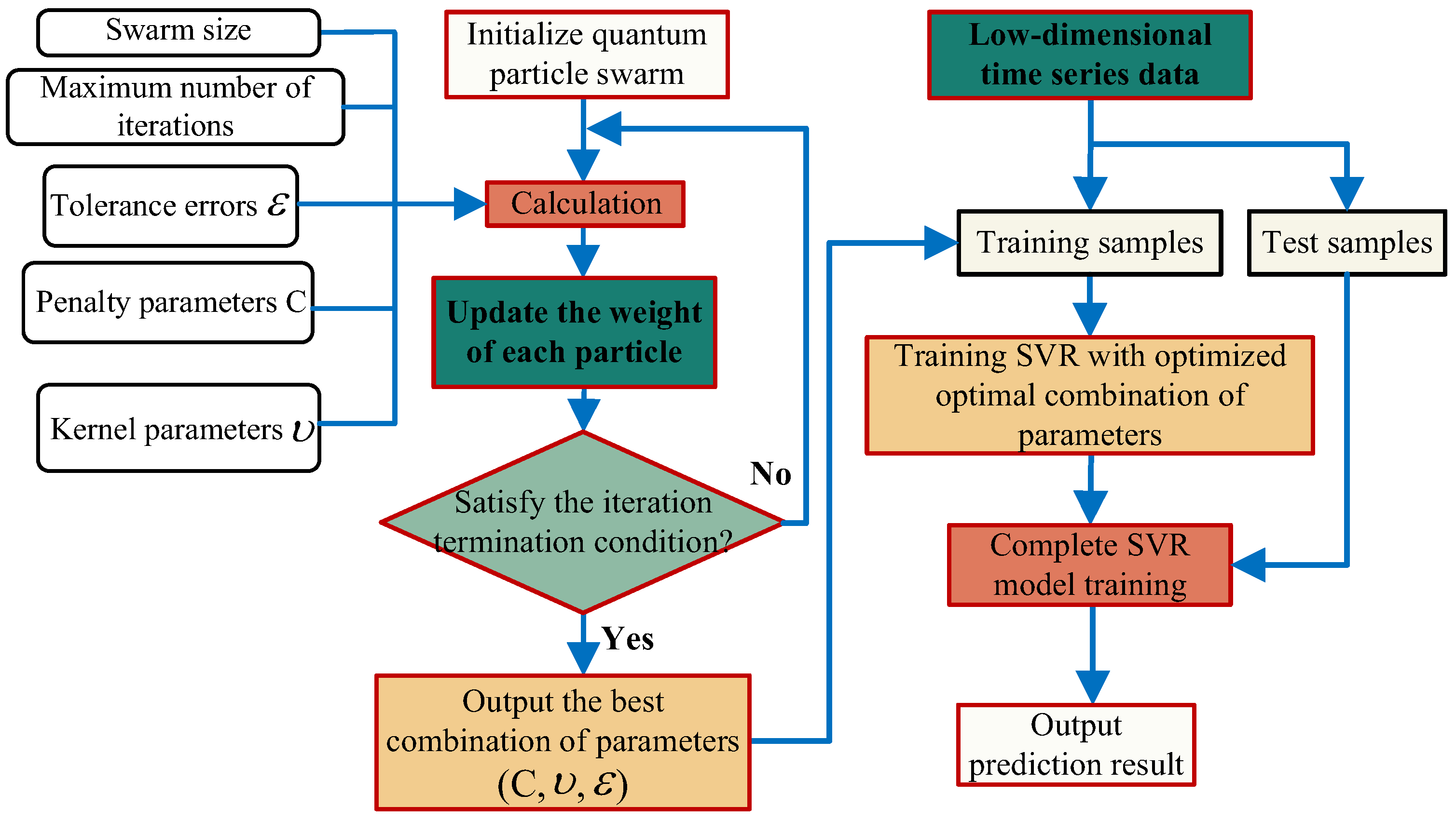
5.2. QPSO Optimization SVR Model Steps

The SVR model’s generalization capacity is influenced by the penalty parameters, C ; kernel parameters, υ ; and tolerance errors, ε . To optimize the SVR model and identify the optimal parameter combination ( C , υ , ε ) , the QPSO algorithm [23,24,25] was used to optimize the model parameters of the SVR load forecasting algorithm, resulting in higher prediction accuracy, as shown in Figure 7.
The specific steps of the QPSO-SVR algorithm are as follows:
(1)
Data preprocessing. Normalize the time series data containing influencing factors, and divide the processed data into training and testing datasets.
(2)
Initialize the quantum particle swarm, such as the swarm size; maximum number of iterations; tolerance errors, ε ; the range of penalty parameters, C; and Gaussian kernel parameters, υ .
(3)
Set the fitness function for QPSO to be mean square error (MSE).
M S E = 1 n i = 1 n y ^ i y i 2
In Equation (15), y ^ i is the predicted value at the i-th iteration and y i is the actual value at the i-th iteration.
(4)
Calculate the optimal positions for each particle in the particle swarm and the global best position using MSE.
(5)
Calculate the average of the optimal positions in the particle swarm and update the particle positions.
(6)
Repeat steps (2) to (5) until the iteration termination condition is met, and output the optimized values of ( c , υ , ε ) .
(7)
Perform load forecasting for electrical, cooling, and heating loads.

6. Load Forecasting Method Based on Composite VTDS Model

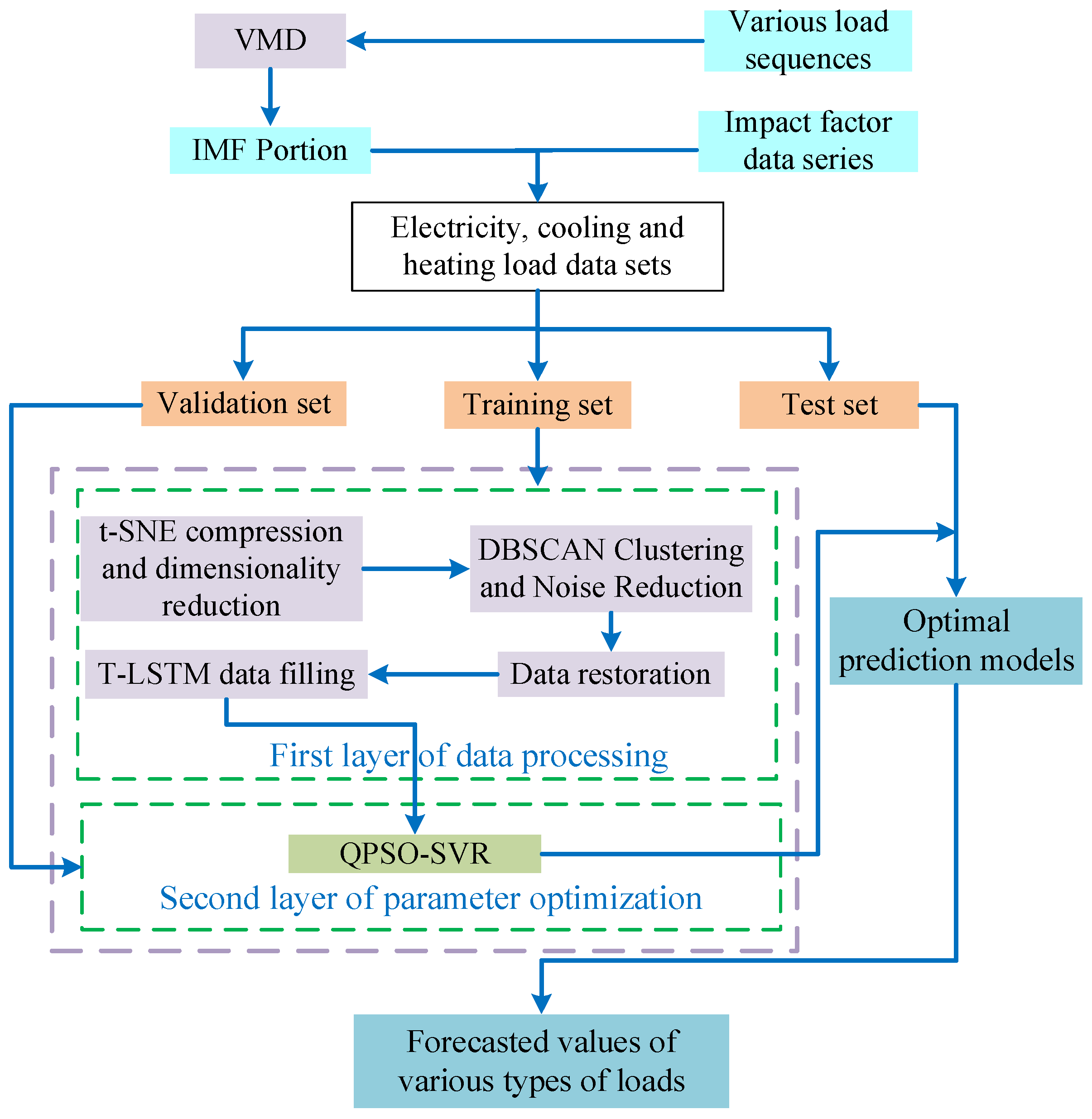
6.1. General Architecture of Composite VTDS Model

Figure 8 presents a comprehensive architecture of the VTDS-based ultra-short-term load forecasting model for IES. The architecture incorporates various components such as VMD, t-SNE, FDBSCAN, and QPSO-SVR. Firstly, VMD is employed to decompose the IES electric, cooling, and heating loads. The resulting IMF components of each load are then combined with time series data that influence IES load prediction, including temperature, carbon emissions, total lighting count, and wind speed. This combination forms a multifactor dataset for each load category. The data are split into a training set, a validation set, and a test set. Subsequently, the multifactor datasets containing IMF components for each load type in the training set undergo the first layer of t-SNE data dimensionality reduction, FDBSCAN clustering, noise reduction, data reduction, and imputation processes to accomplish primary feature selection. The multifactor multi-load validation set, encompassing each IMF component, is fed into the second layer of the QPSO-SVR model for training, aiming to determine the optimal parameters for the model. Finally, the multifactor multivariate load test set is fed into the optimized prediction model for forecasting. The prediction results of each IMF component are combined to obtain the IES load prediction value at the end-user level, which serves to evaluate the effectiveness of the proposed method in this paper.

6.2. Evaluation Indicators

In order to provide a comprehensive assessment of the performance of IES ultra-short-term load forecasting methods, this paper employs several evaluation parameters, namely, root mean square error (RMSE), coefficient of determination (R2), and mean absolute error (MAE). These parameters are utilized to compare and evaluate the load forecasting effectiveness of each model. The definitions of each evaluation parameter are shown in Equations (16)–(18):
(1)
RMSE
R M S E = 1 n i n ( y p r e y i ) 2
(2)
R2
R 2 = 1 i n ( y p r e y i ) 2 i n ( y ¯ y i ) 2
(3)
MAE
M A E = 1 n i n y p r e y
where n is the number of samples in the test set, and y p r e is the predicted value of the electrical, cooling, or heating load at the i-th sample point. y is the actual value of the electrical, cooling, or heating load at the i-th sample point.

7. Calculation Example Analysis

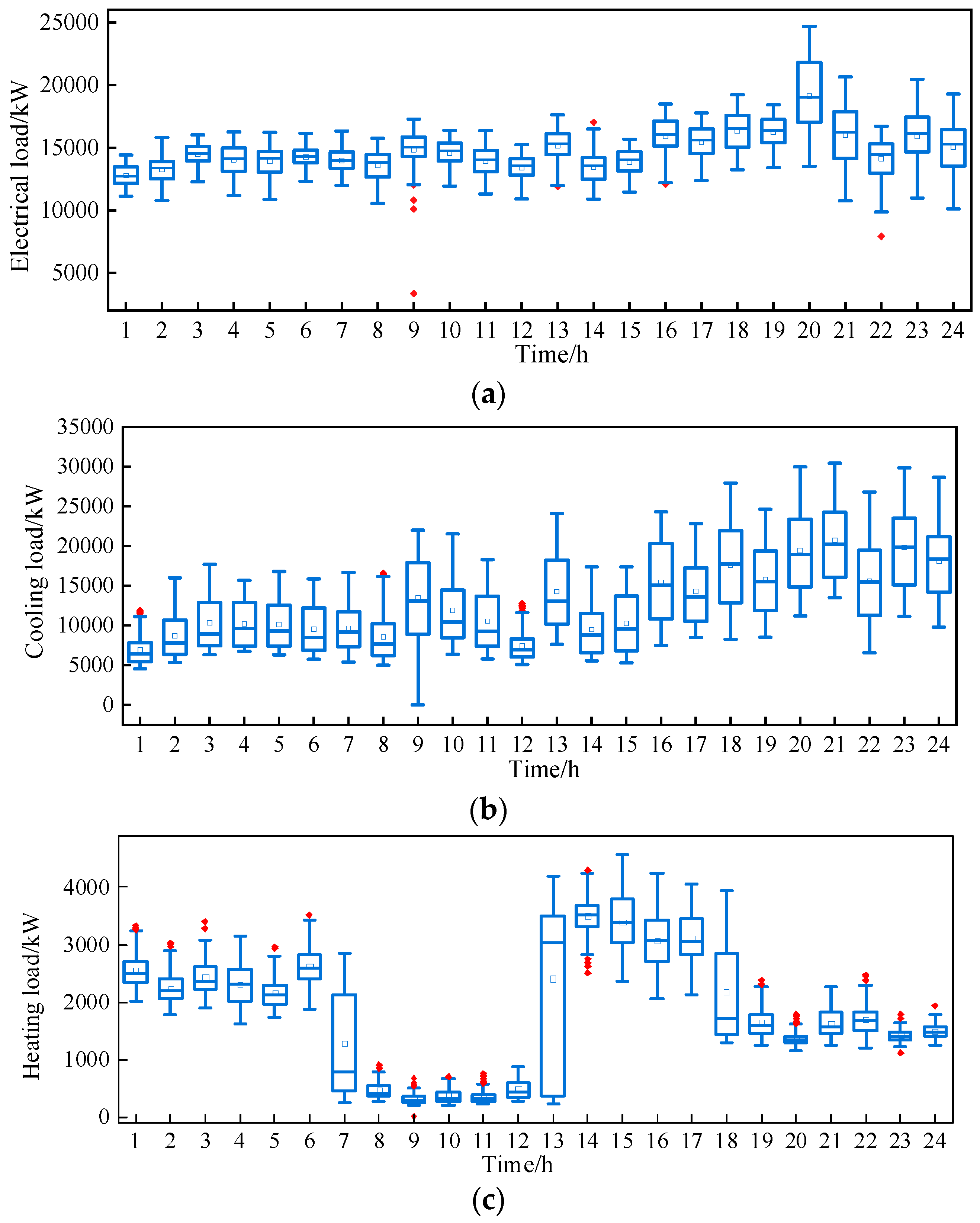
7.1. Experimental Data and Work Platform

In this study, the user-level IES multiple load data were collected from the Tempe campus of Arizona State University in the United States [26]. Weather data were obtained from the National Renewable Energy Laboratory. The data used for experimentation spanned from January to August 2022 and included information on cold load, heat load, electric load, temperature, carbon emissions, and total lighting quantity. The data were sampled at hourly intervals. The test set comprised the data from the last week, while the remaining data were used for training purposes. Three time periods were selected as experimental data: January to February 2022 (winter), March to May 2022 (spring), and June to August 2022 (summer). The data included time series of electric, cooling, and thermal loads, as well as meteorological factors, such as temperature and wind speed. The sampling interval for all datasets was 1 h. Each season (spring, summer, and winter) was separately divided, and the data from 25–31 August 2022, were chosen as the test set, while the remaining data were randomly divided into training and validation sets in a 1:1 ratio. The experimental setup consisted of an Intel Core i7-8750H CPU and 16GB of RAM. The programming was carried out in Python using the PyCharm IDE, with the implementation of the algorithmic models utilizing the PyTorch and learning toolkits.

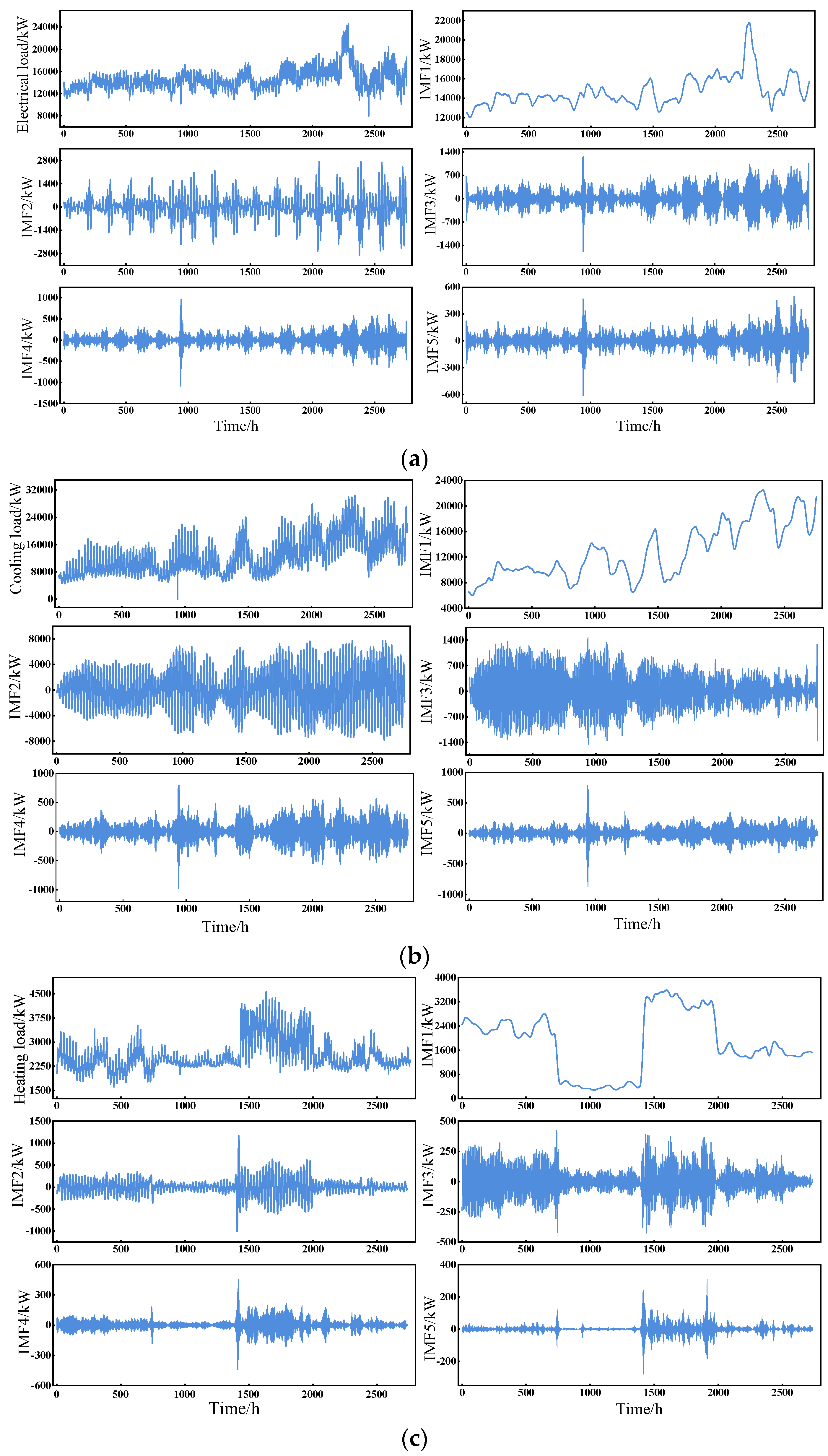
7.2. IES Load Decomposition and Data Series Processing

To enhance the load prediction performance and account for the varying magnitudes of each influencing factor, it is necessary to normalize each component of the input feature vector [27,28]. This normalization process ensures that the data are on a consistent scale and allows for better comparison and analysis. The normalization procedure is carried out as shown in Equation (19).
x i , j a f t e r = x i , j x j min x j max x j min
where x i , j is the value of the j-th component of the i-th sample eigenvector before normalization; x i , j a f t e r is the value of the j-th component of the i-th sample eigenvector after normalization; x j max , x j min are the maximum and minimum values of the j-th component of the eigenvector.
Before decomposing the IES multivariate load using VMD, this paper uses the QPSO Algorithm to determine the optimal decomposition number, K = 5; the quadratic equilibrium parameter; and γ = 1   ×   10 6 is the tolerance error. The IMF curves obtained from the original time series of each load and VMD are shown in Figure 9.
Figure 9 illustrates that IMF1 represents the low-frequency component, capturing the overall trend of various IES load variations. It exhibits a relatively flat pattern and can achieve accurate prediction results. On the other hand, IMF2-IMF5 correspond to the high-frequency components, each exhibiting a concentrated frequency range and representing smoother variations. These components are relatively easier to predict, and their prediction performance can be enhanced through the VMD decomposition process. The experimental results demonstrate that the prediction of IES multiple loads is significantly influenced by meteorological information, energy consumption, and emissions. Therefore, when constructing the features, it is crucial to consider these factors. In this study, the meteorological data provided in the example include seven hourly factors: temperature, air pressure, dew point, wind speed, cloud cover, precipitation, and humidity. Additionally, to incorporate the influence of other factors, such as coal and gas consumption, air quality index, building count, lighting equipment count, greenhouse gas emissions, and day of the week, a total of 14 influencing factors are considered.
For each load, the first six hours of the prediction time are taken into account in the data processing input. The input features consist of each IMF series and the 14 influencing factor series, resulting in a feature dimension of fifteen. Due to the high dimensionality of the data, PCA is employed to determine the feature construction sequence in descending order. Table 2 displays the descending order based on the sum of the principal component contributions exceeding 0.9.
Once the feature construction sequence is determined, the data distribution is evaluated using PCA and t-SNE algorithms [29,30]. The input feature sequence undergoes t-SNE compression and dimensionality reduction operations. Subsequently, the k-means clustering algorithm (K-means) clustering algorithm and fast density-based spatial clustering of applications with noise (FDBSCAN) are employed to compare the effectiveness of noise reduction techniques. The results of PCA-TSNE compression and dimensionality reduction, as well as the comparison between K-means and FDBSCAN noise reduction methods, are depicted in Figure 10, Figure 11 and Figure 12, respectively.
In Figure 10, Figure 11 and Figure 12, the distances and relative positions between data points represent the high-dimensional data of multivariate loads after VMD decomposition and t-SNE compression and dimensionality reduction. The comparison between K-means and FDBSCAN denoising methods illustrates the noise, clustering, and similarity relationships among the high-dimensional data points. When applying the k-means algorithm for noise reduction, it struggles to accurately identify the noise points in the feature sequences used in this paper. Consequently, there are a greater number of isolated noise points after processing. On the other hand, FDBSCAN overcomes the limitations of k-means and demonstrates superior noise reduction performance. Hence, FDBSCAN is utilized for noise reduction in this study. During the data processing operations described above, a data restoration procedure is necessary to restore the original data, which were fragmented. The results of the data restoration are depicted in Figure 13.
Due to climate factors, changes in user demand, equipment failures, or other external factors, load data may exhibit anomalies or missing values. This phenomenon is observed in the data reconstruction process in Figure 13. Meanwhile, the box plots of Figure 14 and Figure 15 provide evidence of the existence of data outliers. The box-and-whisker plot represents the interquartile range (IQR) of the data, which is the middle 50% of the data. The whiskers extend from the edges of the box and represent the data range outside the interquartile range. Data points beyond the whiskers are considered outliers. Data points depicted are as red diamond-shaped boxes in Figure 14 and as green diamond-shaped boxes in Figure 15. Figure 14 displays the hourly box plot for the year 2022, while Figure 15 illustrates the weekly box plot.
In this study, the average value is employed to correct data outliers and address the issue of missing samples by utilizing the information from existing variables. The T-LSTM model is then applied to fill in the missing data in the IMF time series.

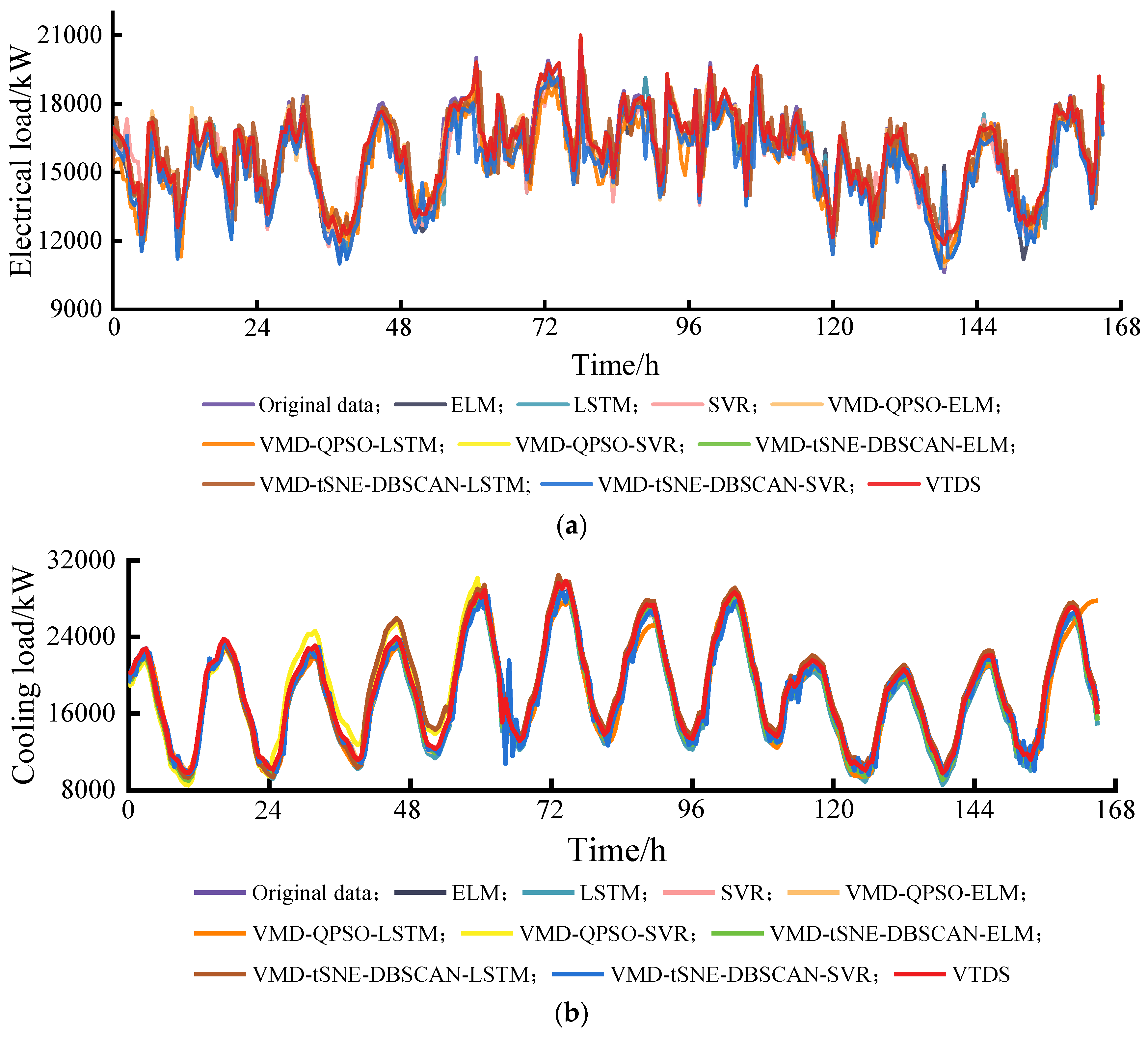
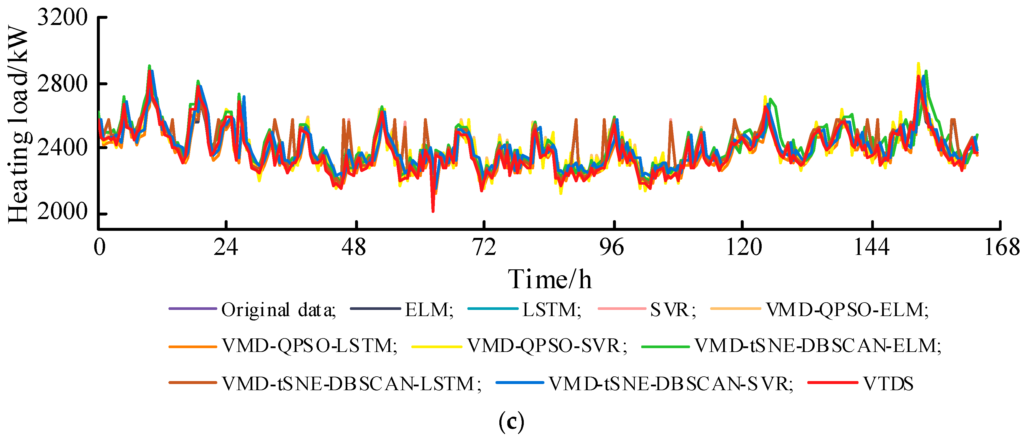
7.3. Results Analysis

The selection of parameters has a significant impact on the IES multivariate load prediction performance of each model. In this paper, the QPSO algorithm is utilized to obtain the optimal hyperparameters for the SVR model, namely, c [ 1 , 2000 ] , v [ 0.0001 , 0.1 ] , and ε [ 0.01 , 0.2 ] . To validate the effectiveness of the VTDS method proposed in this study, various models, including ELM, LSTM, SVR, VMD-QPSO-ELM, VMD-QPSO-LSTM, VMD-QPSO-SVR, VMD-tSNE-DBSCAN-ELM, VMD-tSNE-DBSCAN-LSTM, and VMD-tSNE-DBSCAN-SVR, are compared with the proposed model using different types of load multi-factor datasets as input. Through experiments, it was found that calendar information, such as holidays, has minimal impact on the effectiveness of ultra-short-term load forecasting. Therefore, when constructing the input features, only IES multivariate load and meteorological information are considered. The load in the preceding hours before the prediction moment has a significant impact on the forecasting performance. The experimental results show that considering the preceding 6 h of multivariate load yields the best prediction results. For the VTDS model, the input features include the IMF component values of electric, cooling, and thermal loads for the preceding 6 h and the values of 14 meteorological factors at the prediction moment, resulting in a feature dimension of 29. The load forecasting results for electric, cooling, and thermal loads at 168 time points from 25–31 August 2022, with a 1 h ahead forecast, are shown in Figure 16.
A comparison of each load assessment parameter is shown in Table 3 and Table 4.
From Table 3 and Table 4 and Figure 16, the following can be observed:
(1)
The prediction models lacking VMD decomposition and employing alternative methods for load decomposition exhibit inferior prediction results compared to those utilizing VMD decomposition. Among these machine learning models, considering the overall predictive performance of the dataset, the ELM model shows the highest prediction error with an RMSE value of 618.3691 for the electrical load.
(2)
The introduction of multivariate load decomposition with VMD significantly enhances the performance of the prediction models; particularly, the VMD-tSNE-DBSCAN-SVR combination model showcases notable improvements. The RMSE metric proves to be sensitive to outliers, indicating a substantial difference between the predicted and actual values. The VTDS prediction model achieves an average RMSE value of 44.6277, approximately 0.3 times lower than the lowest value of the other models, showcasing superior performance and effectiveness.
(3)
When considering all the prediction models collectively, the VTDS model exhibits the smallest error in load prediction, as evidenced by the lowest values for evaluation parameters, such as RMSE and MAE. Additionally, the model achieves a high R2 value, indicating excellent prediction accuracy for electric load, second best for cold load, and comparatively weaker performance for heat load.

8. Conclusions

In this paper, a novel approach for ultra-short-term load forecasting in user-level IES is proposed based on VTDS multi-model fusion. The main conclusions and the VTDS multiple load prediction method investigated in this paper encompass the following:
(1)
Adopting VMD to decompose the IES electrical, cooling, and heating load sequences into different intrinsic mode functions (IMFs) reduces the complexity of load time series and lowers the difficulty of prediction.
(2)
During feature construction, the consideration of both the multi-dimensional load and 14 relevant meteorological factors from the preceding 6 h enriches the feature information, which is beneficial for reducing prediction errors.
(3)
Utilizing the QPSO algorithm to optimize the parameters of the SVR model improves the accuracy of the model’s predictions.
(4)
The composite VTDS prediction method, combined with data cleaning algorithms, can enhance feature selection and noise reduction, optimize the time series input of the prediction model, and improve the accuracy of the model’s predictions.
The method proposed in this paper exhibits low sensitivity to temporal and spatial dynamic changes, making it difficult to quickly adapt to sudden variations or new patterns. It also fails to capture dynamic changes within short time intervals. Subsequent research should focus on incorporating spatiotemporal dynamic multi-feature information into the user-level IES ultra-short-term load forecasting problem.

Author Contributions

Conceptualization, S.H., T.L. and Y.X.; methodology, S.H.; software, T.L.; validation, S.H., T.L. and Y.X.; formal analysis, S.H.; investigation, T.L.; resources, S.H. and T.L.; data curation, T.L.; writing—original draft preparation, S.H., T.L. and Y.X.; writing—review and editing, T.L.; visualization, S.H., T.L. and Y.X.; supervision, S.H.; project administration, S.H. All authors have read and agreed to the published version of the manuscript.

Funding

This work was supported by the National Key R&D Program of China (grant no.: 2018YFF01011900).

Data Availability Statement

Not applicable.

Conflicts of Interest

The authors declare no conflict of interest.

Nomenclature

IESIntegrated energy system
VMDVariational mode decomposition
IMFIntrinsic mode function
IMFsIntrinsic mode functions
DBSCANDensity-based spatial clustering of applications with noise
FDBSCANFast density-based spatial clustering of applications with noise
LSTMLong short-term memory
T-LSTMTime-aware long short-term memory
QPSOQuantum particle swarm optimization
ADMMAlternating direction method of multipliers
SVRSupport vector regression
CNNConvolutional neural network
SVMSupport vector machine
ANNArtificial neural network
CARTClassification and regression trees
BiGANBidirectional generative adversarial network
PCAPrincipal component analysis
t-SNET-distributed stochastic neighbor embedding
K-meansK-means clustering algorithm
RMSERoot mean square error
R2Coefficient of determination
MAEMean absolute error
ELMExtreme learning machine

References

  1. Katsaprakakis, D.A.; Zidianakis, G. Optimized dimensioning and operation automation for a solar-combi system for indoor space heating. A case study for a school building in Crete. Energies 2019, 12, 177. [Google Scholar] [CrossRef]
  2. Momen, S.; Nikoukar, J.; Gandomkar, M. Determining Optimal Arrangement of Distributed Generations in Microgrids to Supply Electrical and Thermal Demands using Improved Shuffled Frog Leaping Algorithm. Renew. Energy Res. Appl. 2022, 3, 79–92. [Google Scholar] [CrossRef]
  3. Rad, H.K.; Shariatmadar, H.; Ghalehnovi, M. Simplification through regression analysis on the dynamic response of plates with arbitrary boundary conditions excited by moving inertia load. Appl. Math. Model. 2019, 79, 594–623. [Google Scholar] [CrossRef]
  4. Tan, M.; Liao, C.; Chen, J.; Cao, Y.; Wang, R.; Su, Y. A multi-task learning method for multi-energy load forecasting based on synthesis correlation analysis and load participation factor. Appl. Energy 2023, 343, 121177. [Google Scholar] [CrossRef]
  5. Qiu, B.; Zhang, M.; Li, X.; Qu, X.; Tong, F. Unknown impact force localisation and reconstruction in experimental plate structure using time-series analysis and pattern recognition. Int. J. Mech. Sci. 2019, 166, 105231. [Google Scholar] [CrossRef]
  6. Baliyan, A.; Gaurav, K.; Mishra, S.K. A review of short term load forecasting using artificial neural network models. Procedia Comput. Sci. 2015, 48, 121–125. [Google Scholar] [CrossRef]
  7. Liu, F.; Liu, B.; Zhang, J.; Wan, P.; Li, B. Fault mode detection of a hybrid electric vehicle by using support vector machine. Energy Rep. 2023, 9, 137–148. [Google Scholar] [CrossRef]
  8. Tan, Z.; De, G.; Li, M.; Lin, H.; Yang, S.; Huang, L.; Tan, Q. Combined electricity-heat-cooling-gas load forecasting model for integrated energy system based on multi-task learning and least square support vector machine. J. Clean. Prod. 2019, 248, 119252. [Google Scholar] [CrossRef]
  9. Kang, Q.; Wang, X.; Yuan, Y. Research on regional short-term power load forecasting model and case analysis. Processes 2021, 9, 1617. [Google Scholar] [CrossRef]
  10. Al-Saudi, K.; Degeler, V.; Medema, M. Energy Consumption Patterns and Load Forecasting with Profiled CNN-LSTM Networks. Processes 2021, 9, 1870. [Google Scholar] [CrossRef]
  11. Zhou, D.; Ma, S.; Hao, J.; Han, D.; Huang, D.; Yan, S.; Li, T. An electricity load forecasting model for Integrated Energy System based on BiGAN and transfer learning. Energy Rep. 2020, 6, 3446–3461. [Google Scholar] [CrossRef]
  12. Dai, Y.; Zhao, P. A hybrid load forecasting model based on support vector machine with intelligent methods for feature selection and parameter optimization. Appl. Energy 2020, 279, 115332. [Google Scholar] [CrossRef]
  13. Xu, X.; Meng, Z. A hybrid transfer learning model for short-term electric load forecasting. Electr. Eng. 2020, 102, 1371–1381. [Google Scholar] [CrossRef]
  14. Zhang, Q.; Wu, J.; Ma, Y.; Li, G.; Ma, J.; Wang, C. Short-term load forecasting method with variational mode decomposition and stacking model fusion. Sustain. Energy Grids Netw. 2022, 30, 100622. [Google Scholar] [CrossRef]
  15. Bing, Q.; Shen, F.; Chen, X.; Zhang, W.; Hu, Y.; Qu, D. A Hybrid Short-Term Traffic Flow Multistep Prediction Method Based on Variational Mode Decomposition and Long Short-Term Memory Model. Discret. Dyn. Nat. Soc. 2021, 2021, 4097149. [Google Scholar] [CrossRef]
  16. Granato, D.; Santos, J.S.; Escher, G.B.; Ferreira, B.L.; Maggio, R.M. Use of principal component analysis (PCA) and hierarchical cluster analysis (HCA) for multivariate association between bioactive compounds and functional properties in foods: A critical perspective. Trends Food Sci. Technol. 2018, 72, 83–90. [Google Scholar] [CrossRef]
  17. Tran, T.N.; Drab, K.; Daszykowski, M. Revised DBSCAN algorithm to cluster data with dense adjacent clusters. Chemom. Intell. Lab. Syst. 2013, 120, 92–96. [Google Scholar] [CrossRef]
  18. Bryant, A.; Cios, K. RNN-DBSCAN: A density-based clustering algorithm using reverse nearest neighbor density estimates. IEEE Trans. Knowl. Data Eng. 2017, 30, 1109–1121. [Google Scholar] [CrossRef]
  19. Mou, L.; Zhao, P.; Xie, H.; Chen, Y. T-LSTM: A long short-term memory neural network enhanced by temporal information for traffic flow prediction. IEEE Access 2019, 7, 98053–98060. [Google Scholar] [CrossRef]
  20. Wang, Y.; Du, Y.; Hu, J.; Li, X.; Chen, X. SAEP: A Surrounding-Aware Individual Emotion Prediction Model Combined with T-LSTM and Memory Attention Mechanism. Appl. Sci. 2021, 11, 11111. [Google Scholar] [CrossRef]
  21. Zhou, J.; Zhang, L.; Cao, L.; Wang, Z.; Zhang, H.; Shen, M.; Wang, Z.; Liu, F. Study on Screening Parameter Optimization of Wet Sand and Gravel Particles Using the GWO-SVR Algorithm. Processes 2023, 11, 1283. [Google Scholar] [CrossRef]
  22. Wang, Q.; Yang, R.; Sun, X.; Liu, Z.; Zhang, Y.; Fu, J.; Li, R. The Engine Combustion Phasing Prediction Based on the Support Vector Regression Method. Processes 2022, 10, 717. [Google Scholar] [CrossRef]
  23. Bian, H.; Guo, Z.; Zhou, C.; Wang, X.; Peng, S.; Zhang, X. Research on orderly charge and discharge strategy of EV based on QPSO algorithm. IEEE Access 2022, 10, 66430–66448. [Google Scholar] [CrossRef]
  24. You, Q.; Sun, J.; Pan, F.; Palade, V.; Ahmad, B. Dmo-qpso: A multi-objective quantum-behaved particle swarm optimization algorithm based on decomposition with diversity control. Mathematics 2021, 9, 1959. [Google Scholar] [CrossRef]
  25. Liu, F.; Gao, J.; Liu, H. A fault diagnosis solution of rolling bearing based on MEEMD and QPSO-LSSVM. IEEE Access 2020, 8, 101476–101488. [Google Scholar] [CrossRef]
  26. Zhang, Y.; Shen, H.; Ma, J. Integrated energy system load characteristics analysis and application research. Power Constr. 2018, 39, 18–29. [Google Scholar] [CrossRef]
  27. Xie, D.; Sun, H.; Qi, J. A new feature extraction method based on improved variational mode decomposition, normalized maximal information coefficient and permutation entropy for ship-radiated noise. Entropy 2020, 22, 620. [Google Scholar] [CrossRef]
  28. Xie, D.; Esmaiel, H.; Sun, H.; Qi, J.; Qasem, Z.A.H. Feature extraction of ship-radiated noise based on enhanced variational mode decomposition, normalized correlation coefficient and permutation entropy. Entropy 2020, 22, 468. [Google Scholar] [CrossRef]
  29. Anowar, F.; Sadaoui, S.; Selim, B. Conceptual and empirical comparison of dimensionality reduction algorithms (PCA, KPCA, LDA, MDS, SVD, LLE, ISOMAP, LE, ICA, t-SNE). Comput. Sci. Rev. 2021, 40, 100378. [Google Scholar] [CrossRef]
  30. Liu, H.; Yang, J.; Ye, M.; James, S.C.; Tang, Z.; Dong, J.; Xing, T. Using t-distributed Stochastic Neighbor Embedding (t-SNE) for cluster analysis and spatial zone delineation of groundwater geochemistry data. J. Hydrol. 2021, 597, 126146. [Google Scholar] [CrossRef]
Figure 1. Hourly multi-load distribution in each season. (a) Electrical and cooling load; (b) electrical and heating load; (c) cooling and heating load.
Processes 11 02461 g001
Figure 2. The correlation of variables and multivariate system loads is analyzed using 3D surfaces and pseudo-color maps. (a) Total lightbulbs; (b) temperature; (c) greenhouse gases; (d) total houses.
Processes 11 02461 g002aProcesses 11 02461 g002b
Figure 3. t-SNE algorithm high-dimensional data dimensionality reduction flow chart.
Processes 11 02461 g003
Figure 4. DBSCAN clustering schematic.
Processes 11 02461 g004
Figure 5. FDBSCAN algorithm flow chart.
Processes 11 02461 g005
Figure 6. T-LSTM model.
Processes 11 02461 g006
Figure 7. Flow chart of QPSO-SVR Algorithm.
Processes 11 02461 g007
Figure 8. General architecture diagram of the convergence VTDS model.
Processes 11 02461 g008
Figure 9. A plot of original and VMD curves for each load of the Tempe campus. (a) Electrical load; (b) cooling load; (c) heating load.
Processes 11 02461 g009
Figure 10. PCA-TSNE compression downscaled plot for each load of Tempe campus.
Processes 11 02461 g010
Figure 11. K-means noise reduction figure for each load of Tempe campus.
Processes 11 02461 g011
Figure 12. FDBSCAN noise reduction figure for each load of Tempe campus.
Processes 11 02461 g012
Figure 13. Data reduction graph for each load of Tempe campus. (a) Electrical load; (b) cooling load; (c) heating load.
Processes 11 02461 g013
Figure 14. Hour-level electrical, heat, and cooling load box diagram of 2022. (a) Electrical load; (b) cooling load; (c) heating load.
Processes 11 02461 g014
Figure 15. Weekly electrical, heating, and cooling load box diagram of 2022.
Processes 11 02461 g015
Figure 16. Results for each load forecast of the Tempe campus. (a) Electrical load; (b) cooling load; (c) heating load.
Processes 11 02461 g016aProcesses 11 02461 g016b
Table 1. Pearson correlation matrix for correlation analysis of system multivariate load and influencing factors.
Total LightbulbsTemperatureGreenhouse GasesTotal HousesSystem Load
Total lightbulbs1.000.580.91−0.370.30
Temperature0.581.000.890.32−0.11
Greenhouse gases0.910.891.000.10−0.05
Total houses−0.370.320.101.00−0.39
System load0.30−0.11−0.05−0.391.00
Table 2. PCA descending order table of Tempe campus.
Type of LoadPrincipal Component Contribution RateDescending Order
Electrical load[0.424 0.264 0.249 0.063]3
Cooling load[0.467 0.254 0.181 0.101]4
Heating load[0.329 0.271 0.214 0.186]4
Table 3. Comparison of RMSE parameters for each load of the Tempe campus.
ModelRMSE (Electrical/Cooling/Heating Load)/kWAverage RMSE/kW
ELM618.3691/334.4753/346.5641320.7622
LSTM222.5678/415.8794/323.8393433.1362
SVR129.5528/216.5282/415.9774330.5371
VMD-QPSO-ELM228.7588/112.6572/530.8932290.7697
VMD-QPSO-LSTM314.8551/420.1306/244.2783326.4213
VMD-QPSO-SVR225.9870/417.5440/323.2073322.2461
VMD-tSNE-DBSCAN-ELM317.8189/228.3949/120.6046222.2728
VMD-tSNE-DBSCAN-LSTM429.0997/216.4032/332.6854326.0628
VMD-tSNE-DBSCAN-SVR212.1085/119.8910/97.0682143.0226
VTDS33.2324/46.2816/54.369244.6277
Table 4. Comparison of assessment parameters for each load of the Tempe campus.
ModelMAE (Electrical/Cooling/Heating Load)/kWR2 (Electrical/Cooling/Heating Load)
ELM541.7383/425.3627/338.34640.8662/0.7892/0.8892
LSTM531.0237/764.9110/372.94750.5990/0.7254/0.6301
SVR339.1482/446.1584/529.16940.5770/0.8946/0.8634
VMD-QPSO-ELM445.4997/556.9743/637.03860.8106/0.5366/0.7098
VMD-QPSO-LSTM543.0011/626.4683/735.43650.9215/0.7500/0.8900
VMD-QPSO-SVR435.7677/752.4003/848.58290.6799/0.6480/0.5736
VMD-tSNE-DBSCAN-ELM643.3096/326.0979/438.55510.9607/0.7154/0.5366
VMD-tSNE-DBSCAN-LSTM542.9419/354.1792/666.56410.4739/0.8201/0.7760
VMD-tSNE-DBSCAN-SVR429.3462/233.4583/647.43920.9063/0.8950/0.9261
VTDS64.4961/77.8533/86.59830.9906/0.9823/0.9657
Disclaimer/Publisher’s Note: The statements, opinions and data contained in all publications are solely those of the individual author(s) and contributor(s) and not of MDPI and/or the editor(s). MDPI and/or the editor(s) disclaim responsibility for any injury to people or property resulting from any ideas, methods, instructions or products referred to in the content.

