ROV Sliding Mode Controller Design and Simulation

Abstract

Underwater robots play a vital role in the exploration and development of marine resources and the inspection and maintenance of offshore platforms. In this paper, the motion control technology of ROV is studied, the kinematics and dynamics of ROV are analyzed, the kinematics and dynamics models of ROV are established, and the degrees of freedom of the models are decouple according to the control requirements. The fluid damping coefficient of ROV was obtained using Fluent software, and an ROV control system based on sliding mode variable structure was designed. The saturation function was introduced into the sliding mode controller to reduce the adverse effects of buffeting. The classical PID controller, fuzzy PID controller, and sliding mode controller designed in this paper were simulated and analyzed by Simulink. A semi-physical simulation platform based on Unity3D was established. It can be seen from the simulation results and the pool experiment results that the performance of the sliding mode controller designed in this paper is better than the classical PID controller and the fuzzy PID controller. The sliding mode control method is used to control the ROV motion, which has better control effect and precision.

1. Introduction

Due to the unpredictable marine environment, human understanding of the ocean is still very limited, and the exploitation of marine resources is also hampered. In the underwater environment, as the depth increases, the working environment becomes more and more extreme, and once an accident occurs, it will have disastrous consequences. In order to improve the safety of underwater resource exploration and development, researchers in various countries have developed a variety of underwater operation equipment to replace manual work. Among them, the development and application of underwater detection equipment, especially underwater robots, has become a hot spot in the field of scientific research in various countries. Underwater robots can generally be divided into two categories: one is the cabled underwater robot, commonly known as a remote-operated vehicle (ROV); such robots are operated by remote operators via cables. Another kind is the untethered underwater robot, commonly called the autonomous underwater vehicle (AUV). These robots are underwater platforms that can perform tasks independently. They typically have autonomous navigation, obstacle avoidance, data acquisition, and processing capabilities. Good motion control accuracy is the prerequisite to ensure that the underwater robot can complete the task, which requires the robot to have the ability to quickly approach the target position and maintain stability after reaching the target position. Therefore, motion control technology is always the key field of underwater vehicle research, and the design of control system is also a key part of underwater vehicle development [1,2,3]. The underwater vehicle is a typical nonlinear system, and its mathematical model contains some nonlinear factors, such as fluid resistance and wave interference, which cannot be described by a simple linear model. At the same time, the movements of the various degrees of freedom of the underwater vehicle are coupled with each other, which greatly increases the difficulty of controlling of the underwater vehicle. For the underwater robot system, researchers have tried a variety of control methods and achieved different degrees of control effect, and the main control methods include PID control, fuzzy control, sliding mode control, and neural network control, among others.

PID control is a classical linear system control method that is widely used in industrial control. The principle is to adjust the control quantity according to the size of the current error through the weighting sum of the proportion, integral, and differential links so that the system output is as close as possible to the target value. Fuzzy control is suitable for some nonlinear systems with high complexity and a coupling degree, but it is difficult to establish the exact mathematical model by mathematical method, and the classical control method is difficult to operate. ROV is affected by various factors such as sea waves when moving underwater, so it cannot establish an accurate model and has parameter uncertainty. Therefore, traditional control methods are not suitable for ROV. Sliding mode control is a nonlinear control method that has a good control effect for a system with complex structure and a high nonlinear coupling degree. Its significant advantage is that it has strong robustness to uncertain parameters and external interference. It can realize the stability control of the system by introducing a sliding mode surface, which can realize high-precision control of the system. Therefore, an in-depth study of sliding mode control can achieve accurate and stable ROV control [4,5,6].

In the application process of the sliding mode controller, it is easy for the system to fail to stabilize after reaching the target value, and the controller output always fluctuates in a large range at a higher frequency [7]. This phenomenon is called the buffeting phenomenon, which is because in actual control, the control effect will be affected by various external factors, and the system state may shuttle back and forth on the sliding mode surface. This results in the rapid switching of symbol functions, which leads to chattering. Chattering will lead to increased power consumption and damage to the system hardware. In order to eliminate chattering and improve control performance, the following methods can be used, as shown in

Table 1. Comparison of buffeting elimination methods for sliding mode control.

Method	Advantage	Disadvantage
Select the appropriate sliding surface	Simple and easy to implement, the shape and position of sliding die surface can be adjusted according to the characteristics of the system.	The nonlinear requirements of the system are high, so theoretical analysis and simulation experiments are needed.
Introduce sliding mode surface curve	It can better adapt to the nonlinear characteristics of the system and reduce buffeting.	The curve form needs to be selected according to the system characteristics, which is complicated.
Introducing saturation function	The amplitude of the control input can be limited to reduce buffeting. It is simple and easy to implement.	Large control errors may be introduced.
Introduce adaptive control	The controller parameters can be adjusted according to the dynamic changes of the system to adapt to the uncertain and changing working conditions.	The system needs better modeling and parameter adjustment, and the computational complexity is high.
A sliding mode observer is introduced	System states and unknown disturbances can be estimated, providing more accurate control inputs.	The system needs better modeling and parameter adjustment, and the design and implementation are more complicated.

.

Compared with other methods, methods that introduce saturation functions have the following advantages:

• Simple and easy to implement: The method of introducing saturation function only needs to add saturation function to the control input and does not need to carry out complex modeling and parameter adjustment of the system, which is relatively simple to implement;
• Control input amplitude control: By selecting the appropriate saturation function form and parameters, the amplitude of the control input can be limited, thus reducing buffeting. The parameters of the saturation function can be flexibly adjusted according to the requirements of the system and the control performance to achieve the desired control effect.

Soylu [8] proposed a jitter-free sliding mode control method, which mainly designed adaptive control items instead of discontinuous switching control items. The adaptive control items could continuously compensate for the uncertain effects of the system model, thus eliminating jitter. However, this method is complicated and has many control parameters, so it is difficult to realize in practice. Huang [9] adopted the double-closed-loop sliding mode control method to improve the ground anti-jamming ability during ROV movement and designed a continuous function as a switching control item to reduce the jitter problem of sliding mode control. However, this method does not consider the influence of uncertain factors of the ROV model. Fossen [10] used a multi-variable sliding mode control in ROV dynamic positioning, which requires a high accurate estimation of system parameters, which may present certain difficulties in practical application.

Based on the nonlinear ROV model, a sliding mode controller based on saturation function was designed to solve the problem that ROV motion control is susceptible to external interference and buffeting, considering the uncertainty of modeling and the influence of model interference and buffeting. The six-degrees-of-freedom mathematical model of ROV was established by analyzing the dynamics and kinematics of ROV. According to the design requirements, the model was simplified, and the degree of freedom was decoupled. The decoupled model was used for the subsequent controller design. Fluent software was used to numerically simulate the fluid-damping coefficients of the ROV for snorkeling movement and yaw movement. The first- and second-order fluid-damping coefficients were obtained and fed into the sliding mode controller. The sliding mode controller was improved by using continuous saturation function instead of sign function, and a boundary layer was designed. Continuous control was adopted in the boundary layer, and normal sliding mode control was adopted outside the boundary layer so as to eliminate the effect of buffeting. A MATLAB simulation experiment and Unity3D semi-physical simulation verified the effectiveness of the method, and the ROV experiment was carried out in the pool environment, and the experimental data were good, meeting the application requirements.

2. ROV Mathematical Model Establishment

The mathematical model of the ROV is mainly divided into two parts, namely the kinematics model and dynamics model. The kinematic model is used to describe the motion state of ROV in water, including position, attitude, speed, acceleration, etc. The dynamics model is used to describe the force and torque of the ROV when it moves in water and the change of its motion state [11].

2.1. Establishment of Motion Model

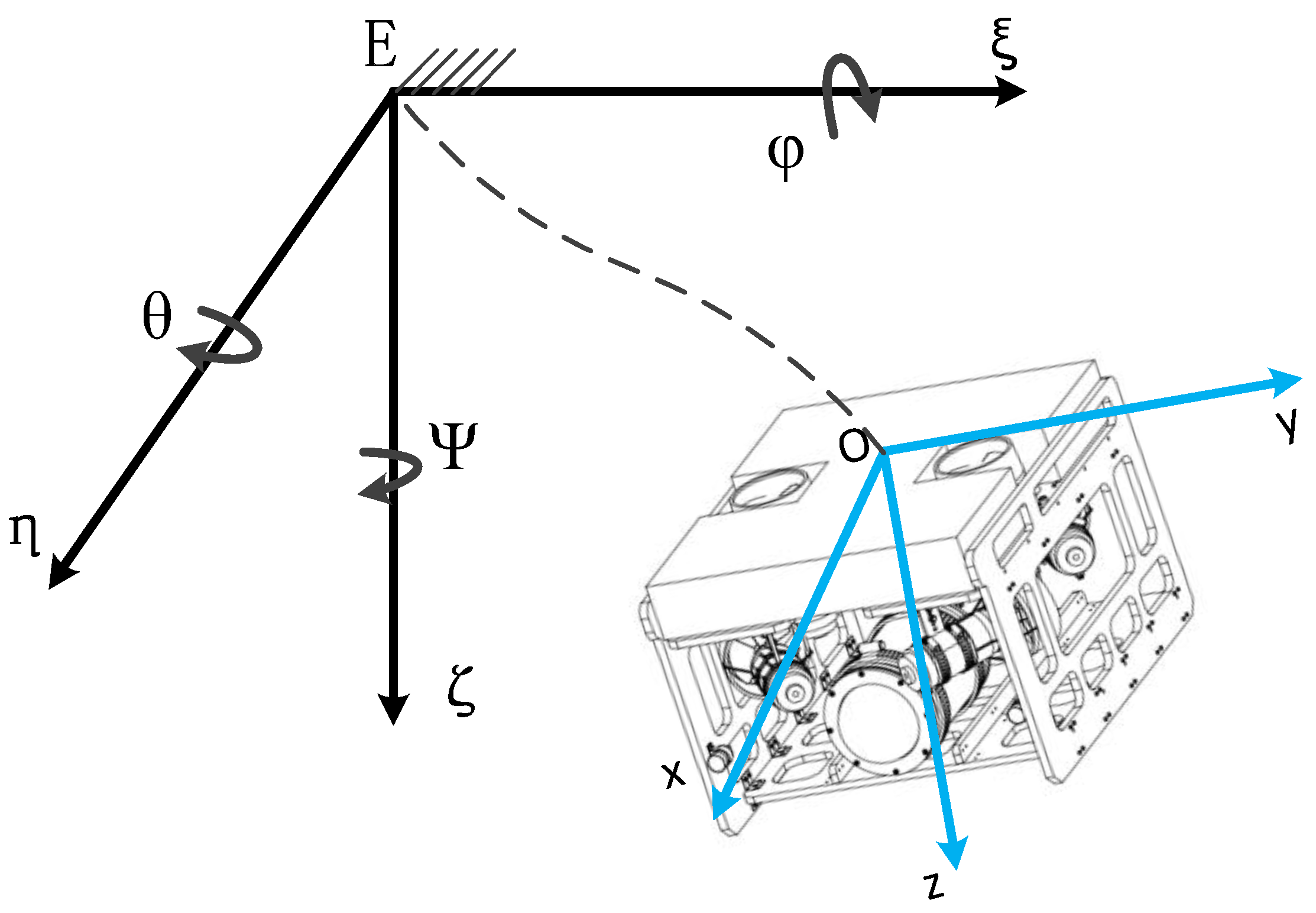
According to the coordinate system recommended by the International Towing Tank (ITTC) and the terminology bulletin of the Marine Engineering Society (SNAME), the geodetic coordinate system E and the ontology coordinate system O were established. Both coordinate systems follow the right-hand rule. The position parameter is expressed by the position coordinate (x, y, z) of the origin of the body coordinate system in the geodetic coordinate system, and the attitude parameter is expressed by the attitude angle (φ, θ, Ψ) of the body coordinate system rotating relative to the geodetic coordinate system. The linear velocity of the ROV along the three axes of the body coordinate system is expressed by (u, v, w), and the angular velocity of the ROV rotating around the three axes is expressed by (p, q, r) [12]. The diagram of the coordinate system is shown in Figure 1.

The transformation relationship between the geodetic coordinate system and the ontology coordinate system is as follows:

$$v_{\mathrm{E}}=J\cdot v_{\mathrm{O}}$$

(1)

Formula:

$v_{\mathrm{E}}$ is the linear velocity vector of the ROV in the geodetic coordinate system;

$v_{\mathrm{O}}$ is the linear velocity vector of the ROV in the body coordinate system;

$J$ is the transformation matrix in the two coordinate systems.

$$J=\left(\begin{array}{cc}{J}_1& 0_{3\ast 3}\\ 0_{3\ast 3}& J_2\end{array}\right)$$

(2)

$$J_1=\left(\begin{array}{ccc}\cos \theta \cos \psi & -\cos \phi \sin \psi +\sin \phi \sin \theta \cos \psi & \sin \phi \sin \psi +\cos \phi \sin \theta \cos \psi \\ \cos \theta \sin \psi & \cos \phi \cos \psi +\sin \phi \sin \theta \sin \psi & -\sin \phi \cos \psi +\cos \phi \sin \theta \sin \psi \\ -\sin \theta & \sin \phi \cos \theta & \cos \phi \cos \theta \end{array}\right)$$

(3)

$$J_2=\left(\begin{array}{ccc}1& \sin \phi \tan \theta & \cos \phi \tan \theta \\ 0& \cos \phi & -\sin \phi \\ 0& \sin \phi \sec \theta & \cos \phi \sec \theta \end{array}\right)$$

(4)

The linear velocity and angular velocity between the geodetic coordinate system and the body coordinate system can be transformed by the two matrices J₁ and J₂, and the complete kinematics equation of the ROV can be obtained by integrating them, as shown below [13].

$$\left(\begin{array}{cc}{J}_1& 0_{3\ast 3}\\ 0_{3\ast 3}& J_2\end{array}\right)\left(\begin{array}{l}{v}_1\hfill \\ v_2\hfill \end{array}\right)=\left(\begin{array}{l}{\dot{\eta }}_1\hfill \\ {\dot{\eta }}_2\hfill \end{array}\right)$$

(5)

$$v_1=\left(\begin{array}{l}u\hfill \\ v\hfill \\ w\hfill \end{array}\right)v_2=\left(\begin{array}{l}p\hfill \\ q\hfill \\ r\hfill \end{array}\right){\eta }_1=\left(\begin{array}{l}x\hfill \\ y\hfill \\ z\hfill \end{array}\right){\eta }_2=\left(\begin{array}{l}\phi \hfill \\ \theta \hfill \\ \psi \hfill \end{array}\right)$$

(6)

$$\begin{array}{l}\left(\begin{array}{cccccc}\cos \theta \cos \psi & -\cos \phi \sin \psi +\sin \phi \sin \theta \cos \psi & \sin \phi \sin \psi +\cos \phi \sin \theta \cos \psi & 0& 0& 0\\ \cos \theta \sin \psi & \cos \phi \cos \psi +\sin \phi \sin \theta \sin \psi & -\sin \phi \cos \psi +\cos \phi \sin \theta \sin \psi & 0& 0& 0\\ -\sin \theta & \sin \phi \cos \theta & \cos \phi \cos \theta & 0& 0& 0\\ 0& 0& 0& 1& \sin \phi \tan \theta & \cos \phi \tan \theta \\ 0& 0& 0& 0& \cos \phi & -\sin \phi \\ 0& 0& 0& 0& \sin \phi \sec \theta & \cos \phi \sec \theta \end{array}\right)\left(\begin{array}{l}\mathrm{u}\\ \mathrm{v}\\ \mathrm{w}\\ \mathrm{p}\\ \mathrm{q}\\ \mathrm{r}\end{array}\right)=\left(\begin{array}{c}\dot{x}\\ \dot{y}\\ \dot{z}\\ \dot{\phi }\\ \dot{\theta }\\ \dot{\psi }\end{array}\right)\\ \end{array}$$

(7)

2.2. Dynamic Model

The dynamics modeling of ROV is mainly based on Newton’s law and momentum theorem. The resultant force of ROV can be decomposed into hydrodynamic force, static force, driving force, and force caused by external interference. The force on the ROV along the three axes is expressed by (X, Y, Z), and the torque around the three axes is expressed by (K, M, N). The modes of ROV movement in six degrees of freedom are defined as advance and retreat, transverse movement, snorkeling, rolling, pitching, and turning as follows:

$$\tau =g+{\tau }_H+{\tau }_T+f$$

(8)

Formula:

$g$ is the static force of the ROV, including gravity and buoyancy force;

${\tau }_H$ is the fluid power received by ROV, including inertial and viscous hydrodynamic power;

${\tau }_T$ is the driving force of ROV, mainly provided by thrusters;

$f$ is the interference force caused by the ROV due to factors such as wave impact and umbilical cable interference.

Before modeling, according to the ROV design requirements, in order to facilitate the calculation, the following simplification is made:

(1)

The ROV’s center of gravity must coincide with the origin O of the moving coordinate system, that is, r_G = (0, 0, 0);

(2)

During the design process, the ROV’s gravity and buoyancy are equalized by trim;

(3)

The ROV center of buoyancy coincides with the center of gravity during the design of the structure, that is, r_B = (0, 0, 0);

(4)

Since the ROV body is approximately symmetric, the non-diagonal elements on the mass matrix M_RB and the additional mass matrix M_A can be ignored, and the corresponding Coriolis centripetal force matrix can be simplified, where M_RB is the inertia matrix of ROV, and M_A is the additional mass matrix;

(5)

Since the movement speed of an ROV in operation is usually slow, the coefficient higher than secondary in fluid power is ignored, and only the primary and secondary coefficients are retained.

When an ROV moves in water with multiple degrees of freedom, cross-coupling will occur between the degrees of freedom, and the faster the running speed, the stronger the coupling effect, which makes the process of solving the ROV’s motion state very complicated. Therefore, the mathematical model of the ROV needs to be decoupled by degrees of freedom in practical applications. The six-degrees-of-freedom movements of ROV were decoupled and decomposed into six single-degree-of-freedom movements. The six-degrees-of-freedom dynamics equation of the ROV can be simplified to Equation (9), and the motion parameters are defined in

Table 2. Definition of ROV motion parameters.

Motion Parameter	x-Axis	y-Axis	z-Axis
Position	x	y	z
Posture	φ	θ	Ψ
Linear velocity	u	v	w
Angular velocity	p	q	r
Force	X	Y	Z
Moment of force	K	M	N
Moment of inertia	Ix	Iy	Iz

.

$$\left\{\begin{array}{l}\left(m-X_{\dot{u}}\right)\dot{u}+\left(X_u+X_{u\left|u\right|}\left|u\right|\right)u=X\\ \left(m-Y_{\dot{v}}\right)\dot{v}+\left(Y_v+Y_{v\left|v\right|}\left|v\right|\right)v=Y\\ \left(m-Z_{\dot{w}}\right)\dot{w}+\left(Z_w+Z_{w\left|w\right|}\left|w\right|\right)w=Z\\ \left(I_x-K_{\dot{p}}\right)\dot{p}+\left(K_p+K_{p\left|p\right|}\left|p\right|\right)p=K\\ \left(I_y-M_{\dot{q}}\right)\dot{q}+\left(M_q+M_{q\left|q\right|}\left|q\right|\right)q=M\\ \left(I_z-N_{\dot{r}}\right)\dot{r}+\left(N_r+N_{r\left|r\right|}\left|r\right|\right)r=N\end{array}\right.$$

(9)

3. Solution of Fluid Damping Coefficient

In the mathematical model, there are some unknown parameters, namely the fluid-damping coefficient. In this paper, Fluent software was first used to conduct fluid simulation, and the obtained simulation data were sorted and fitted to obtain the first-order and second-order fluid-damping coefficients of two degrees of freedom, namely, snorkeling motion and yaw motion, which were used for the subsequent controller design [14,15].

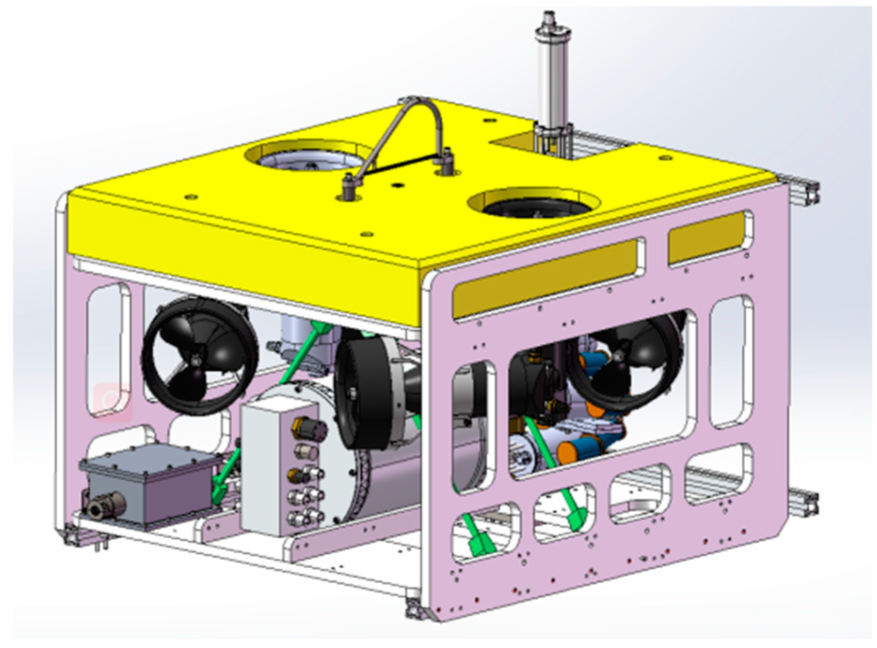
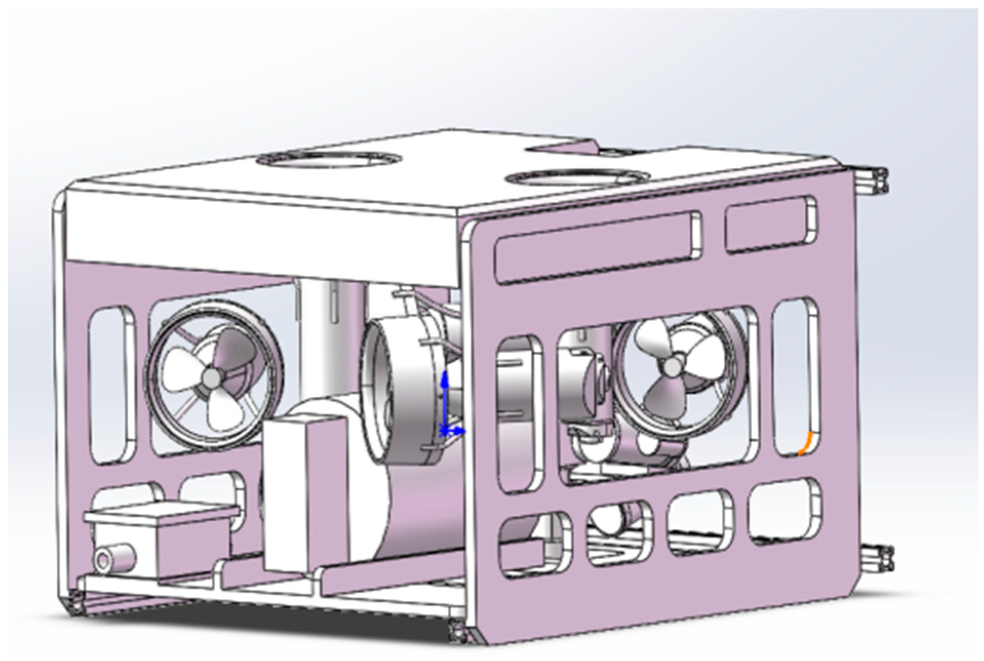
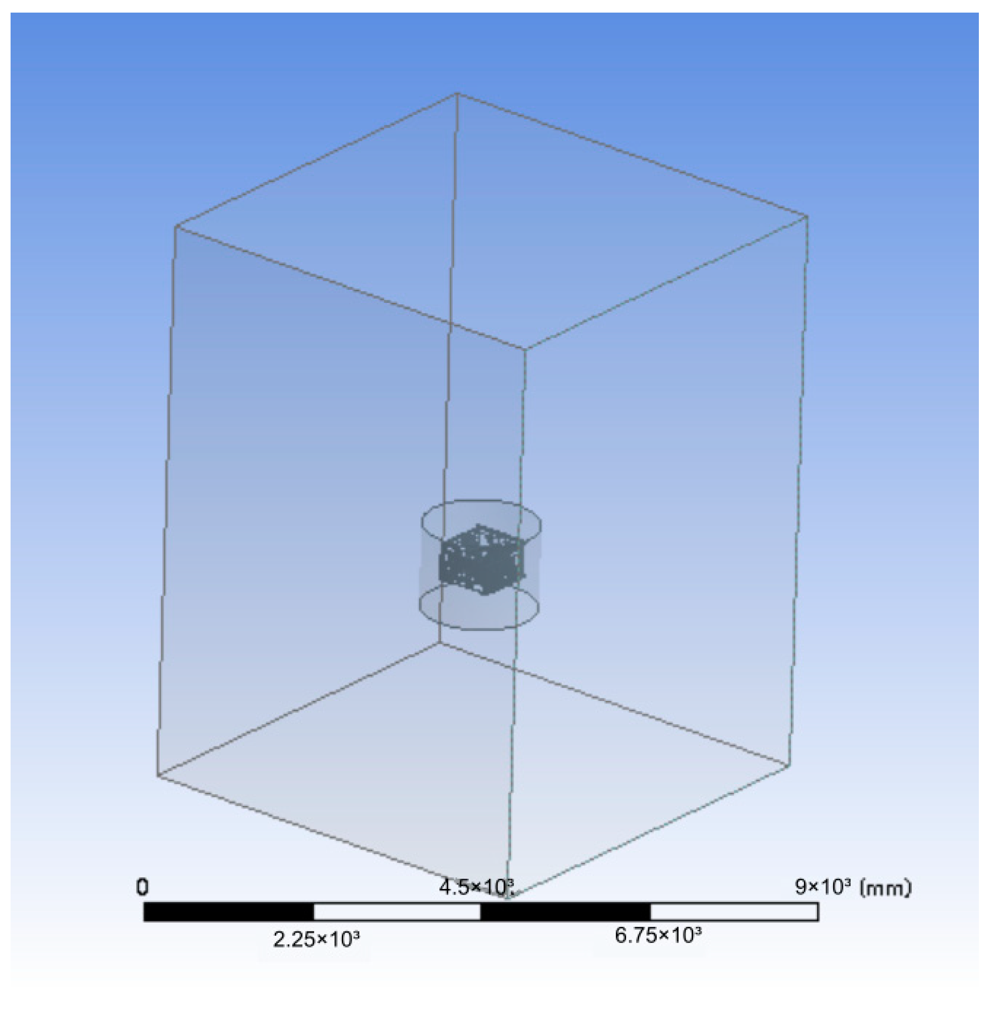
Firstly, the ROV three-dimensional model was processed. The original model structure contains a variety of parts and complex surfaces with complex structures. Direct simulation will cause difficulty in grid division and excessive calculation and even make completion of the calculation impossible. The principle of model simplification is to retain the main features while ignoring the complex and small structure. 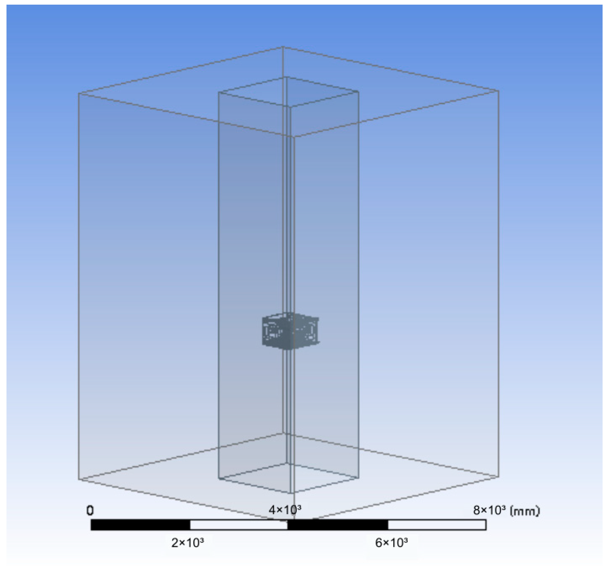On the basis of the original model, the simplified model in this paper ignores various holes, pinion motors, recovery hooks, and various connecting parts made due to the installation of pendent equipment.The original model is shown in Figure 2 and the simplified model is shown in the Figure 3

In this paper, the simulated fluid domain is divided into two parts: the outer fluid domain and the inner fluid domain. In general, the model size of the fluid domain should be more than three times that of the ROV to reduce the impact of the wall. The size of the ROV in this paper is 800 mm × 750 mm × 600 mm (length × width × height), and the size of the external fluid domain is defined as 6000 mm × 6000 mm × 8000 mm. The initial ROV position is 3000 mm away from the bottom of the outer fluid domain. The cuboid structure with a fluid domain of 2000 mm × 2000 mm × 8000 mm and set in the linear motion simulation is shown in Figure 4. For the simulation of rotating motion, the inner fluid domain was set as a cylindrical structure, with a bottom circle radius of 800 mm and a height of 1200 mm, as shown in Figure 5.

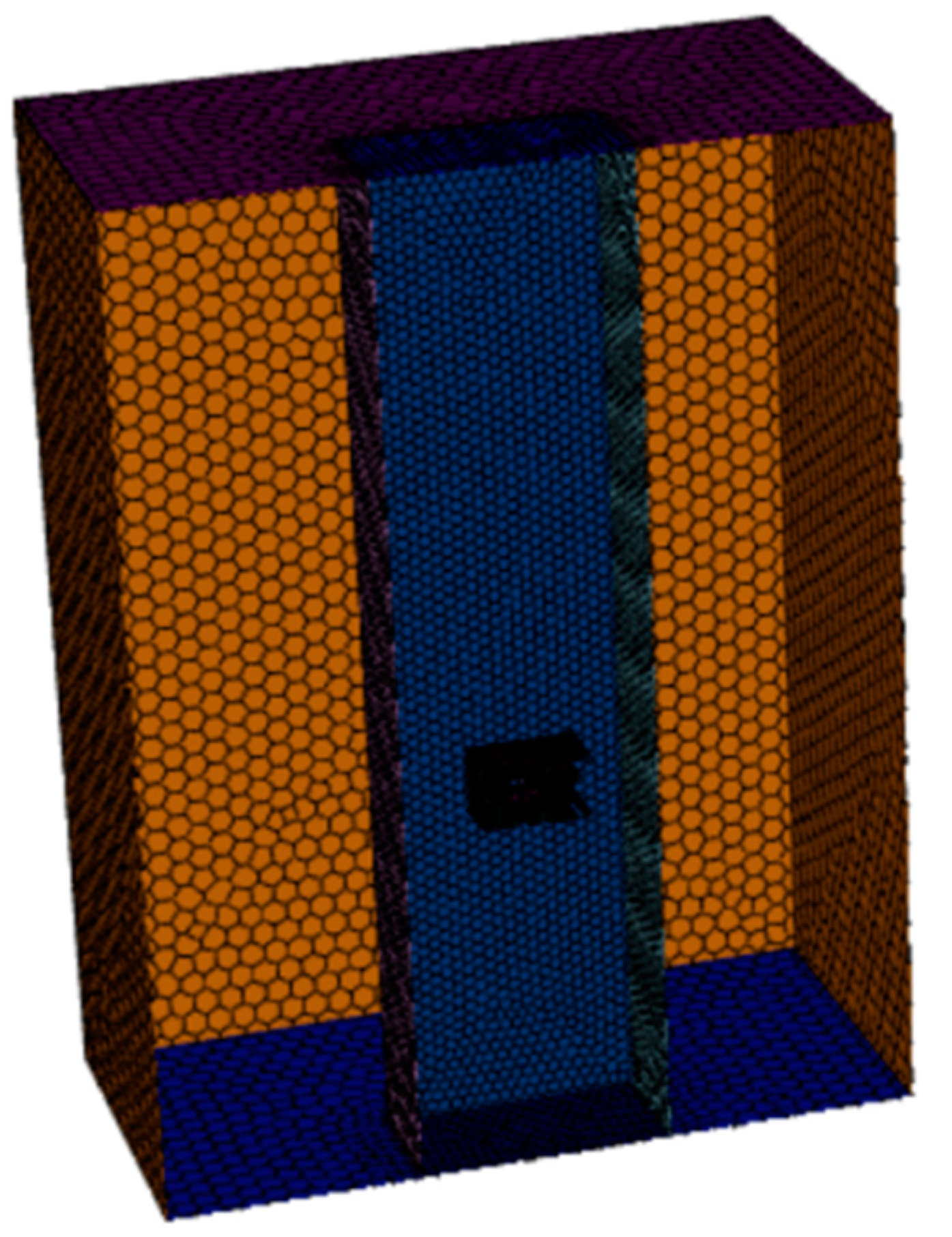
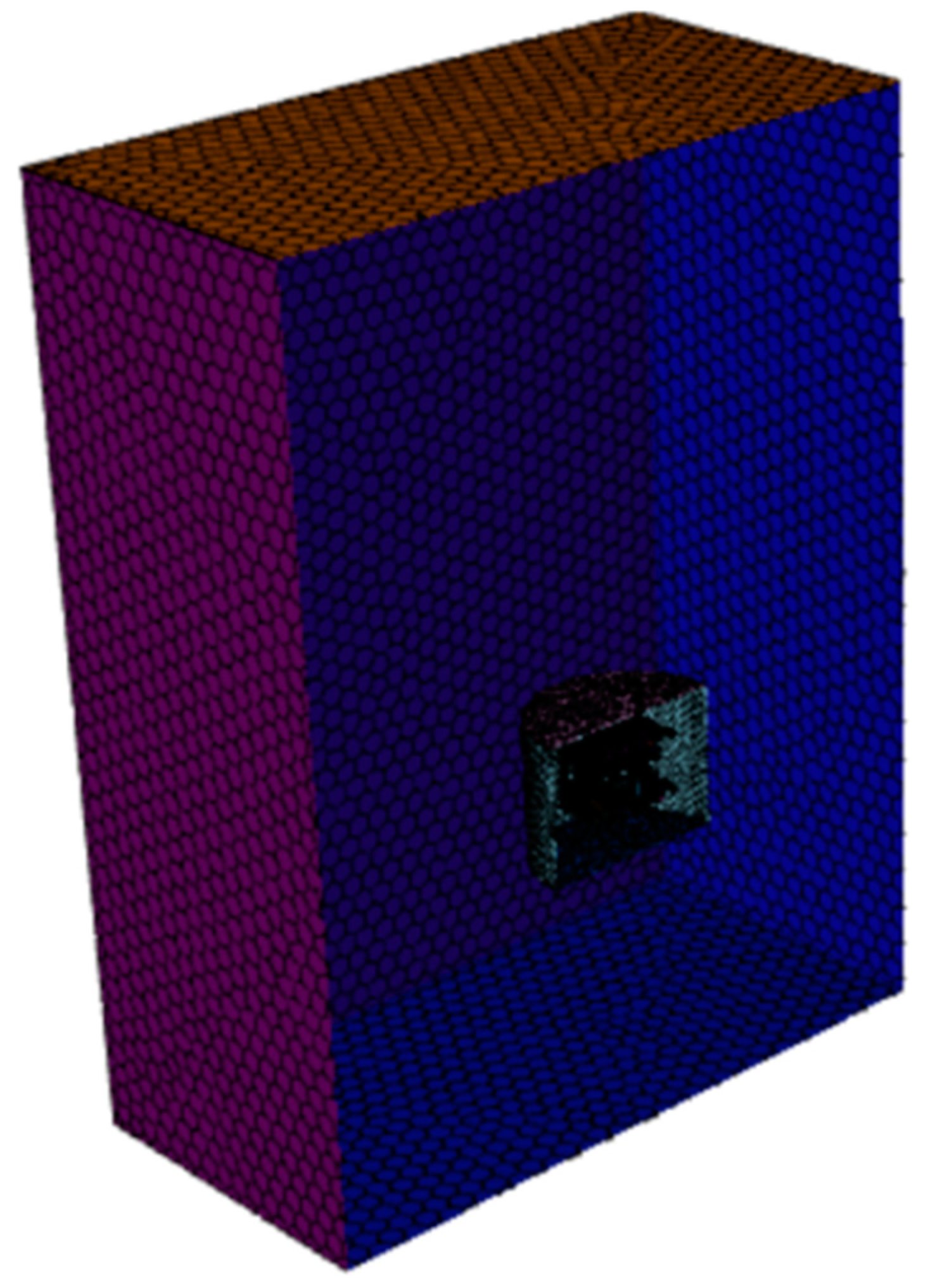
Next, the model was meshed, and polyhedral meshes are used in this paper. The number of grids will affect the simulation results. Insufficient grids will lead to distortion of the calculation results, while excessive grids will slow down the calculation speed but have little impact on the calculation results. Other papers have verified the grid number independence of ROV fluid simulation, and it can be concluded that when the number of grids reaches more than 1 million, the impact on the calculation results can be ignored. In this study, the method of mixed mesh division was used to encrypt the internal fluid domain, and the size of the encrypted mesh was set to 0.001 m. After encryption, the number of mesh in the snorkeling direct motion simulation fluid domain was 2,811,957, and the number of mesh in the turning and rotating simulation fluid domain was 2,794,722 [16]. The model meshing results of linear motion and rotational motion are shown in Figure 6 and Figure 7.

For each degree of freedom, 10 sets of simulation with different speeds were carried out, with a total of 20 working conditions. The force and torque data of ROV at different speeds and motion modes were obtained. According to the simulation data, it can be seen that with the increase of the robot’s motion speed, the resistance and resistance moment of the robot also increase, and their relationship is similar to the quadratic function relationship. MATLAB 2021a software was then used to curve fit the data.

Using a quadratic function form to fit the data, the curve equation of resistance fitting for snorkeling movement can be obtained as follows:

$$f(w)=346.5w^2-0.4461w+0.142$$

(10)

The fitting curve equation of the resistance moment of the heading movement is as follows:

$$f(r)=19.89r^2+0.08433r-0.004357$$

(11)

The first- and second-order fluid-damping coefficients of ROV snorkeling and turning movements can be obtained as shown in the

Table 3. Table of fluid-damping coefficients.

First-Order Fluid-Damping Coefficient	Numerical Value	Second-Order Fluid-Damping Coefficient	Numerical Value
$Z_w$	−0.4461	$Z_{w\left|w\right|}$	346.5
$N_r$	0.08433	$N_{r\left|r\right|}$	19.89

.

4. Sliding Mode Controller Design

The conventional nonlinear system of the controlled object can be expressed by the following equations:

$$\left\{\begin{array}{l}{\dot{x}}_1(t)=x_2(t)\hfill \\ {\dot{x}}_2(t)=f(x_1,x_2)+bu(t)+d_z\hfill \end{array}\right.$$

(12)

Formula:

$x_1,x_2$ is the state variable of the system;

$f(x_1,x_2)$ is the nonlinear term of the system;

$u$ is the input of the control system;

To control the gain, $b$ is a known bounded function or a fixed value;

$d_z$ represents the internal interference of the system and the external uncertainties.

In this paper, the decoupling of the two-degrees-of-freedom models of snorkeling and turning over can be transformed, and the following equations can be obtained, which, respectively, represent the single-degree-of-freedom model of an ROV with the two degrees of freedom of snorkeling and turning over, as shown in Formulas (13) and (14).

$$\begin{array}{c}\left\{\begin{array}{l}\dot{z}=w\hfill \\ \dot{w}=b_Z{\tau }_Z+f(w)w+d_Z\hfill \end{array}\right.\\ \begin{array}{c}{b}_Z=\frac{1}{m-Z_{\dot{w}}}\\ f(w)=-\frac{Z_w+Z_{w\left|w\right|}\left|w\right|}{m-Z_{\dot{w}}}\end{array}\end{array}$$

(13)

$$\begin{array}{c}\left\{\begin{array}{l}\dot{\psi }=r\hfill \\ \dot{r}=b_N{\tau }_N+f(r)r+d_N\hfill \end{array}\right.\\ \begin{array}{c}{b}_N=\frac{1}{I_z-N_{\dot{r}}}\\ f(r)=-\frac{N_r+N_{r\left|r\right|}\left|r\right|}{I_z-N_{\dot{r}}}\end{array}\end{array}$$

(14)

The design of the sliding mode controller can be divided into two steps: firstly, we select the appropriate sliding mode surface and secondly, design the control law that can obtain a system approach to the sliding mode surface in a limited time and at the same time eliminate the negative effects of buffeting as much as possible [17,18].

The sliding mode surface set in this paper is shown in Formula (13), where the order of the highest derivative contained in the sliding mode surface is called the order of the sliding mode surface. The higher the order of the sliding mode surface, the higher the control accuracy of the system, but at the same time, the calculation will be more complicated. The sliding mode surface designed in this paper is a first-order sliding mode surface.

$$s=ce+\dot{e}=0$$

(15)

where c is a constant, and c > 0.

$$e(t)=x_{1d}-x_1$$

(16)

$$\dot{e}(t)={\dot{x}}_{1d}-{\dot{x}}_1={\dot{x}}_{1d}-x_2$$

(17)

$$\ddot{e}(t)={\ddot{x}}_{1d}-{\dot{x}}_2$$

(18)

Therefore,

$$\dot{s}=c\dot{e}+\ddot{e}$$

(19)

$$\dot{s}=c({\dot{x}}_{1d}-x_2)+({\ddot{x}}_{1d}-{\dot{x}}_2)$$

(20)

Among them:

$e$ is the error between the target value and the actual value;

$x_{1d}$ is the target displacement and also the target position;

$x_1$ is the actual displacement or actual position;

${\dot{x}}_{1d}$ is the derivative of the target displacement, which is also the target velocity, and the derivative of the actual displacement, which is also the actual velocity;

$\dot{e}$ is the derivative of the error, which is also the velocity error.

The approach law of the sliding mode controller designed in this paper selects the exponential approach law as follows [19,20]:

$$\dot{s}=-\epsilon \cdot \mathrm{sgn}(s)-ps,\begin{array}{l}\hfill \end{array}\epsilon >0,p>0$$

(21)

sgn(s) is a symbolic function whose expression is as follows:

$$\mathrm{sgn}(s)=\left\{\begin{array}{l}1\begin{array}{cc}& s>0\end{array}\\ 0\begin{array}{cc}& s=0\end{array}\\ -1\begin{array}{cc}& s<0\end{array}\end{array}\right.$$

(22)

Substituting the formula yields the following:

$$-\epsilon \cdot \mathrm{sgn}(s)-ps=c\dot{e}+\ddot{e}$$

(23)

$$-\epsilon \cdot \mathrm{sgn}(s)-ps=c({\dot{x}}_{1d}-x_2)+({\ddot{x}}_{1d}-{\dot{x}}_2)$$

(24)

$$-\epsilon \cdot \mathrm{sgn}(s)-ps=c({\dot{x}}_{1d}-x_2)+({\ddot{x}}_{1d}-f(x_1,x_2)-bu(t)-d_z)$$

(25)

The sliding mode controller model can be obtained as follows:

$$u(t)=\left[c({\dot{x}}_{1d}-x_2)+({\ddot{x}}_{1d}-f(x_1,x_2)-d_z)+\epsilon \cdot \mathrm{sgn}(s)+ps\right]/b$$

(26)

For the specific controller model of the two degrees of freedom of the heading and depth of the ROV in this paper, Equations (13) and (14) are substituted into Equation (26), respectively, as follows [21,22]:

$${\tau }_Z=\left[c({\dot{x}}_{1d}-x_2)+({\ddot{x}}_{1d}-f(w)w-d_Z)+ps+\epsilon \cdot \mathrm{sgn}(s)\right]/b_Z$$

(27)

$${\tau }_N=\left[c({\dot{x}}_{1d}-x_2)+({\ddot{x}}_{1d}-f(r)r-d_N)+ps+\epsilon \cdot \mathrm{sgn}(s)\right]/b_N$$

(28)

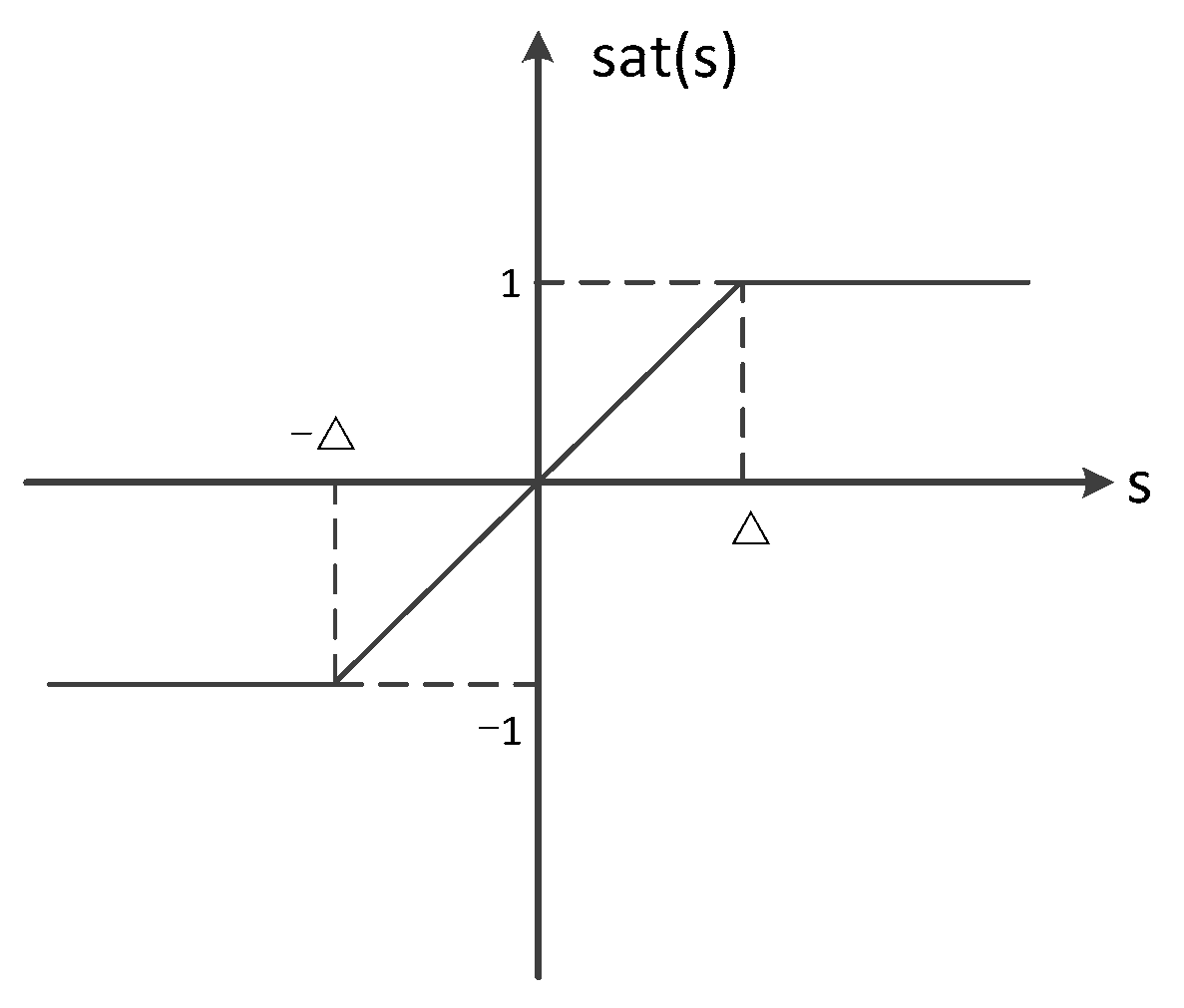
In order to eliminate the bucket vibration of the sliding mode controller, the saturation function is introduced to reduce the buffeting phenomenon and enhance the robustness and stability of the system. In this method, a boundary layer is designed. Continuous control is adopted in the boundary layer, and a normal sliding mode control is adopted outside the boundary layer to eliminate the effect of buffeting. The schematic diagram of saturation function is shown in Figure 8.The saturation function is as follows:

$$sat(s)=\left\{\begin{array}{l}1 s>\Delta \\ ks \left|s\right|\le \Delta ,k=1/\Delta \\ -1 s<-\Delta \end{array}\right.$$

(29)

The controller model of heading and depth two degrees of freedom after adding the saturation function is shown as follows:

$${\tau }_Z=\left[c({\dot{x}}_{1d}-x_2)+({\ddot{x}}_{1d}-f(w)w-d_Z)+ps+\epsilon \cdot \mathrm{sat}(s)\right]/b_Z$$

(30)

$${\tau }_N=\left[c({\dot{x}}_{1d}-x_2)+({\ddot{x}}_{1d}-f(r)r-d_N)+ps+\epsilon \cdot \mathrm{sat}(s)\right]/b_N$$

(31)

5. Simulation Analysis

This paper focuses on the simulation analysis of two degrees of freedom of ROV movement, namely snorkeling degrees of freedom along the z-axis and turning degrees of freedom around the z-axis. For each degree of freedom, two kinds of motion were simulated, respectively, namely the motion of fixed depth and fixed bow and the trajectory tracking motion of variable value. The performance of the sliding mode controller was verified by comparing with the simulation results of the classical PID controller and fuzzy PID controller.

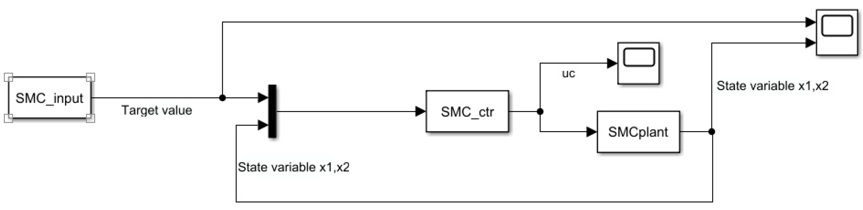
To establish the controller model in Simulink, first, we added the corresponding script file name and required external parameters in the S-function module setting so as to establish the corresponding relationship between the S-function module and the script file. Next, the input, controller, and controlled object were connected; a complete closed-loop control model was established; and the state changes were observed with an oscilloscope. In the debugging process, the degree of freedom can be changed by changing the model parameters of the param.m file, and different target values can be set by changing the input.m file to simulate different working conditions. The built simulation model of sliding mode control is shown in Figure 9 [23,24]:

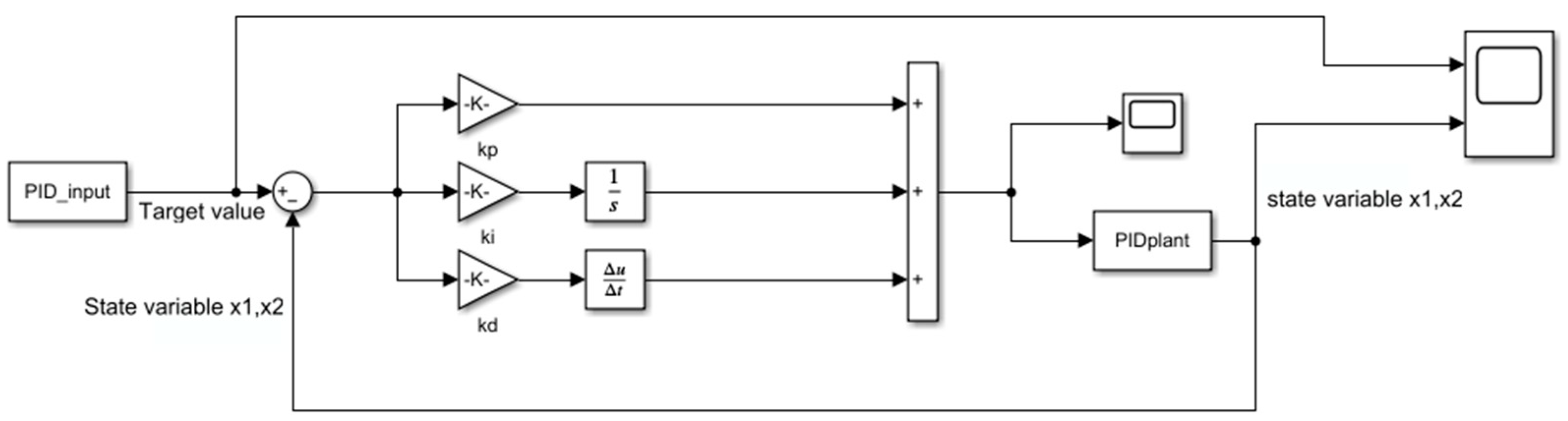
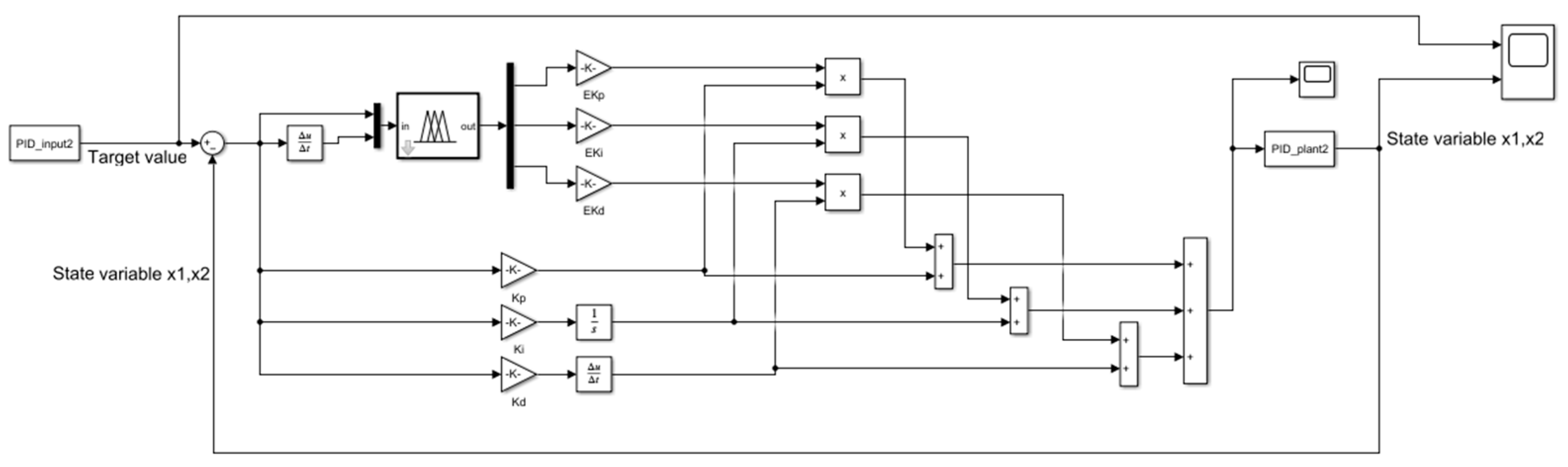
According to the principle of the classical PID control and fuzzy PID control, the simulation model was established, respectively. The input and controlled object were still established by S-function module, and the controller model was built by the built-in module of the system. The complete classical PID and fuzzy PID simulation models are shown in Figure 10 and Figure 11:

5.1. Snorkeling Simulation

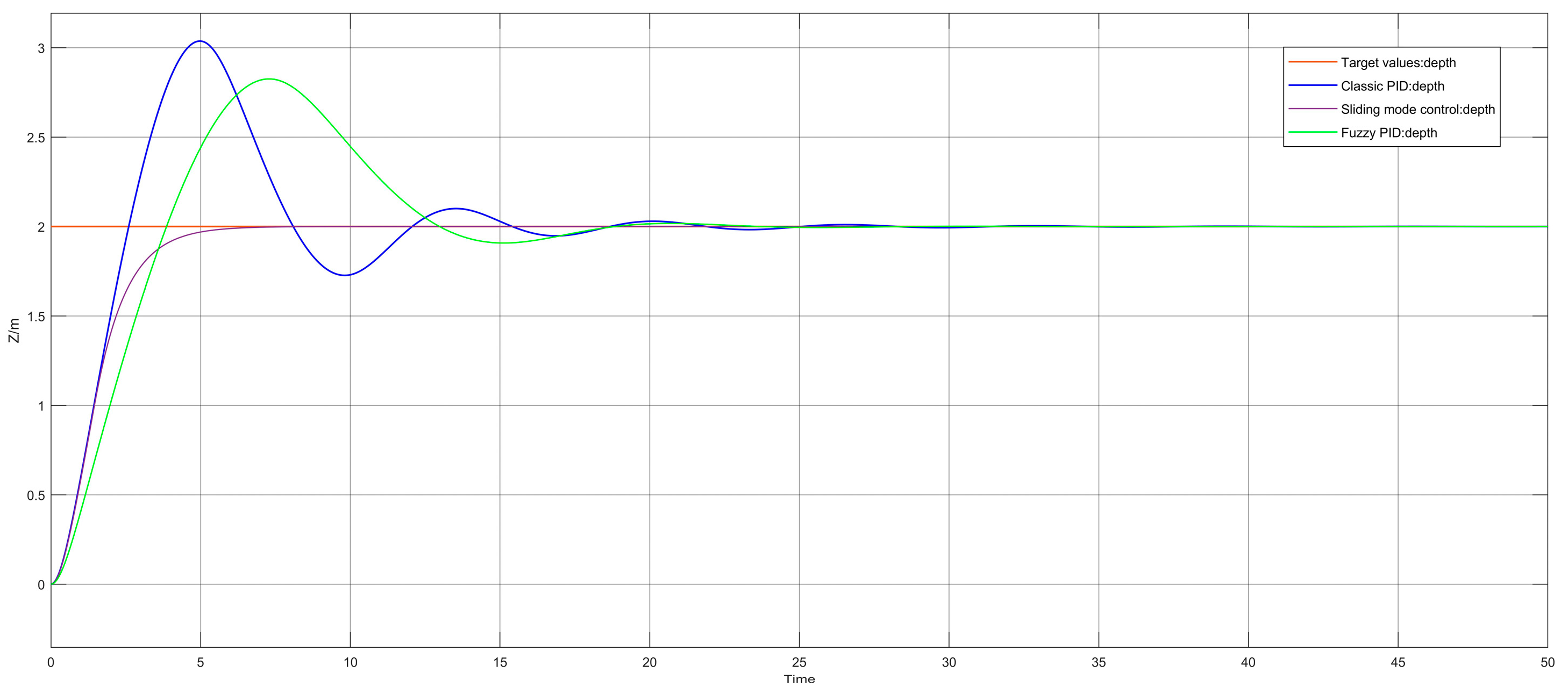
ROV snorkeling motion simulation is the direct motion simulation along the z-axis of the robot. The simulation under this degree of freedom was divided into two parts. The first part was to set a fixed depth value so that the ROV can quickly reach the target value from zero initial state and maintain stability and simulate the depth-determination function of the ROV in the operation. The initial state depth of the controlled object was set to 0 m, the speed to 0 m/s, the simulation time to 50 s, the step length to 0.01 s, and the fixed-depth target value to 2 m. The simulation was carried out using three algorithms, namely classical PID, fuzzy PID, and sliding mode control, and the control effect was shown as the follows in Figure 12.

Next, we observed the above images and analyzed the control effect of each controller. The stability time of classical PID controller is the longest, which is about 23.8 s. The stability time of fuzzy PID is slightly shorter than that of the classical PID controller, about 18.5 s [23,24]. The sliding mode controller has the shortest stability time, about 8.1 s. Due to the upper limit of the thruster’s thrust output in practical application, the output range of the controller was set within ±300 in simulation, which increases the system stability time to a certain extent. From the perspective of overshoot, the maximum deviation of the classical PID controller is 0.8, and the overshoot is 40%. The maximum deviation of fuzzy PID controller is 0.67, and the overshoot is 33.5%. The sliding mode controller has no obvious overshoot because of its control characteristics. To summarize, it can be seen that the three controllers can finally stabilize the system in the simulation of directly moving fixed depth, but the control effect is different, among which the sliding mode controller has the best effect, the fuzzy PID effect is second, and the PID effect is the worst.

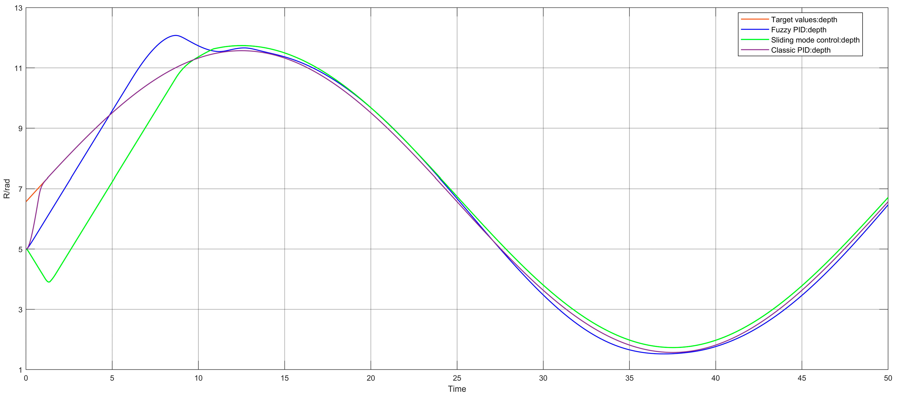
The second part of the simulation was to set a target value function that changes with time so that the ROV can track the changing target value and simulate the operation state of the ROV for continuous position changes. The depth and speed of the initial ROV state were set to 6.5 m and 0 m/s, the simulation time was set to 50 s, and the step length was set to 0.01 s. The varying target depth value is expressed by a sinusoidal function, whose formula is as follows:

$${\mathrm{Z}}_{\mathrm{d}}=A\sin \left(\frac{2\pi }{T}t\right)+B\hspace{1em}\hspace{1em}\hspace{1em}A=5,T=50,B=5$$

(32)

Three control algorithms were used for simulation, and the control effect is shown in Figure 13:

According to the analysis of the simulation results, the stability time of the classical PID is about 14.2 s, that of the fuzzy PID is about 10.0 s, and that of the sliding mode controller is about 7.5 s. From the tracking effect, the fuzzy PID and sliding mode controller have better tracking effects, and there is always a steady-state error between the classical PID and the target value. To summarize, both the sliding mode controller and fuzzy PID meet the control requirements in the direct dynamic simulation of variable depth, and the sliding mode controller is better than the fuzzy PID controller.

5.2. Simulation of Heading Motion

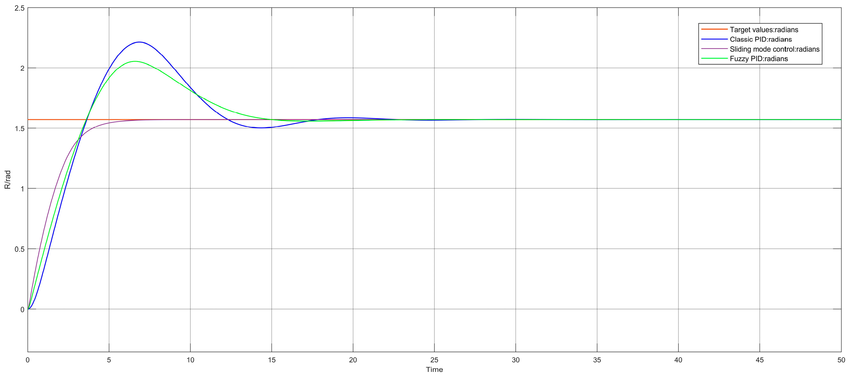
Next, the ROV heading motion simulation, that is, the simulation of rotation around the robot’s z-axis, was also divided into two parts under this degree of freedom: fixed target value angle and variable target value angle. In the first part, we set a fixed target heading value to simulate the heading function of ROV in operation. In the heading simulation, the ordinate unit adopted the radian system, and the target value was set at 90°, which was converted to about 1.57 rad. Next, we selected the positive direction, set the initial state heading of the ROV to 0, the angular velocity to 0 rad/s, the simulation time to 50 s, and the step length to 0.01 s, respectively, and used three control algorithms for simulation. The control effect is shown in Figure 14.

It can be seen from the simulation image that the output value of the controller was also set within ±300 in the heading motion simulation. In terms of stability time, the classical PID controller has the longest stability time, about 15.5 s; the stability time of the fuzzy PID controller is slightly higher than that of the classical PID controller, about 17.5 s. The stability time of the sliding mode controller is 7.5 s, which is significantly lower than that of the classical PID and fuzzy PID. From the perspective of overshoot, the maximum deviation of the classical PID controller is 0.48 rad, and the overshoot is about 30.6%. The maximum deviation of the fuzzy PID controller is 0.41 rad, and the overshoot is about 26.1%. The sliding mode controller has no obvious overshoot. In summary, it can be seen that the effect of the fuzzy PID controller is similar to that of the classical PID controller in the rotation simulation of the fixed heading target value, while the effect of the sliding mode controller is significantly better than the two in terms of stability time and overshoot.

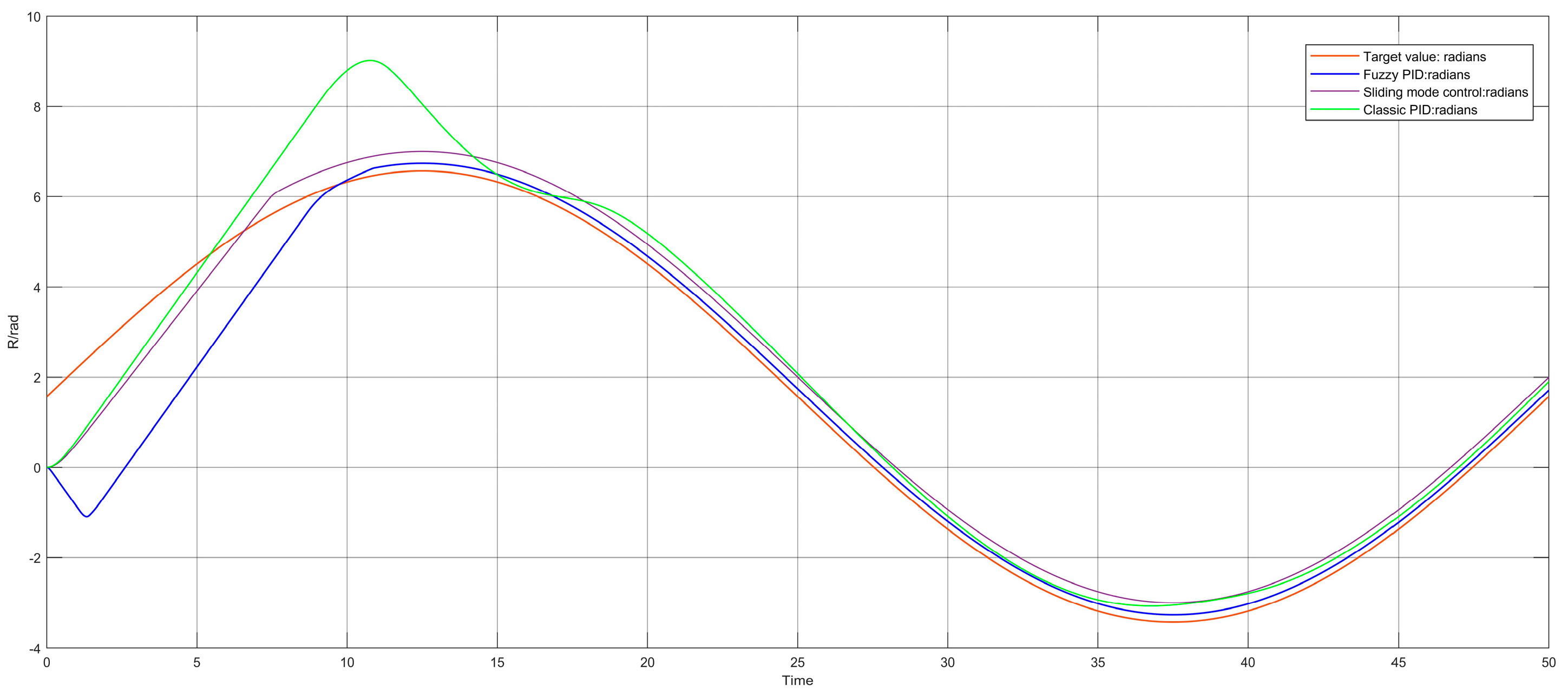
The second part of the rotation simulation was to set a heading target value that changes with time and also make the target heading value change in the way of a sine function so as to simulate the operating state of the ROV when requiring continuous steering. The heading and angular velocity of the initial ROV state were set to 0 and 0 rad/s respectively; the simulation time was set to 50 s; and the step length was set to 0.01 s. Three control algorithms were used for simulation, and the control effect is shown in the Figure 15.

It can be seen from the simulation image that the sliding mode controller can track the changing target value better after a period of adjustment, and the stability time is 6.2 s. Both the fuzzy PID controller and the classical PID controller have different degrees of steady-state error, in which the fuzzy PID controller has a large deviation at the initial time and gradually approaches the target value after 10 s of adjustment. The classic PID controller gradually approaches the target value after about 14 s of adjustment. Comparing the effect of the three control algorithms, it can be seen that the effect of the sliding mode controller designed in this paper is better than that of the fuzzy PID and classical PID in the rotation simulation of changing the heading value of the target.

5.3. Unity3D Simulation Environment Test

Based on the three-dimensional simulation system of Unity3D, the system test has a higher degree of visualization and can observe the control effect more intuitively. In the 3D simulation system, the ROV model and underwater physical environment model were established according to the physical characteristics of the real world so that the simulation environment was closer to the real world. The motion state of the ROV body can be shown in the 3D simulation system [25].

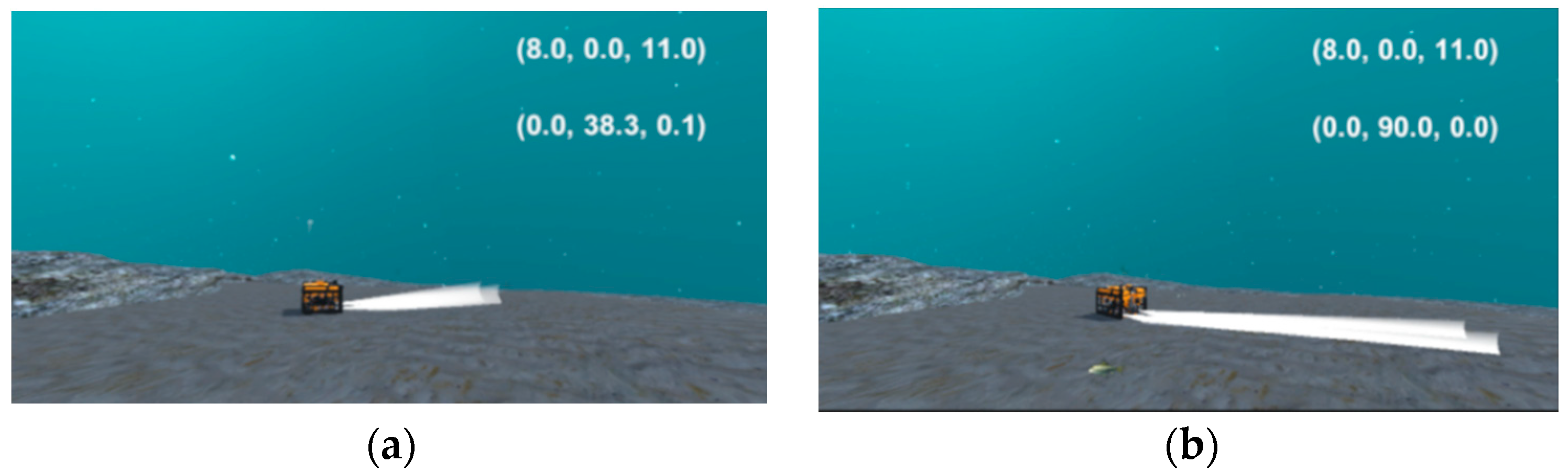
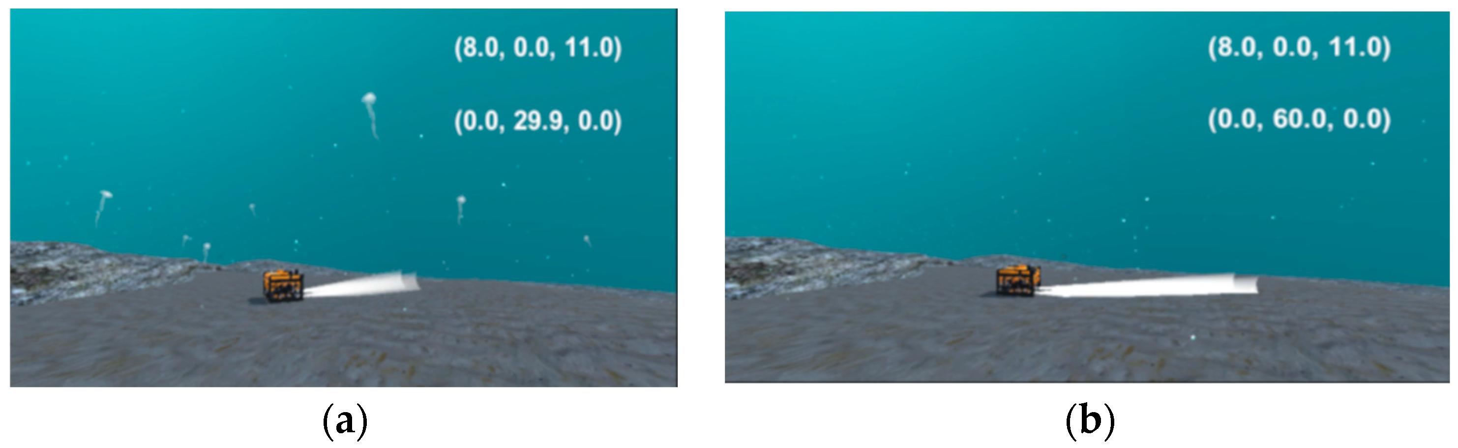
Firstly, the heading motion function was tested in the 3D simulation system, the target angle was set to 90°, and the animation effect and the coordinate transformation in the upper right corner were observed after input of the angle target value, as shown in the following figure, in which Figure 16a shows the image during the change process, and Figure 16b is the image after the ROV reached the target value and stabilized. After the ROV starts to move, its y-axis angle coordinate gradually increases from 0.0° and finally stabilizes at 90.0°, with a stabilization time of about 14.1 s. From the simulation animation effect and coordinate changes, it can be seen that the alignment test basically meets the control requirements.

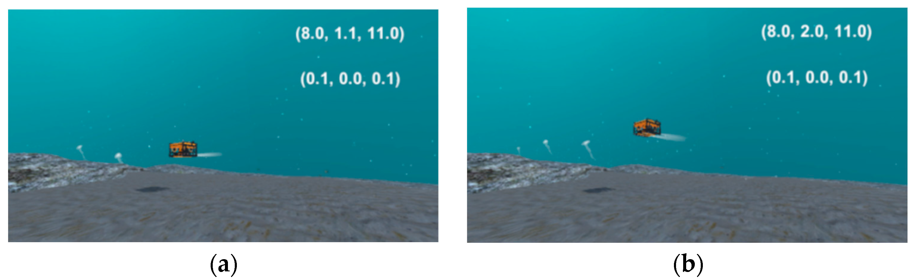
In this paper, two sets of test results with target values of 30° and 60° were selected, and the stability time is 12.0 s and 13.3 s, respectively, with an error of less than 0.1°. The test effect diagram is shown in Figure 17. It can be seen that the test results of several calibration simulations meet the control requirements.

Next, the ROV depth setting function was tested, and the target depth was set at 2.0 m. Animation effect and coordinate transformation in the upper right corner were observed. The y-axis position coordinate gradually changed from 0.0 to 2.0 and finally stabilized at 2.0, with a stabilization time of about 11.9 s, as shown in Figure 18. It can be seen from the results that the fixed-depth simulation basically meets the control requirements.

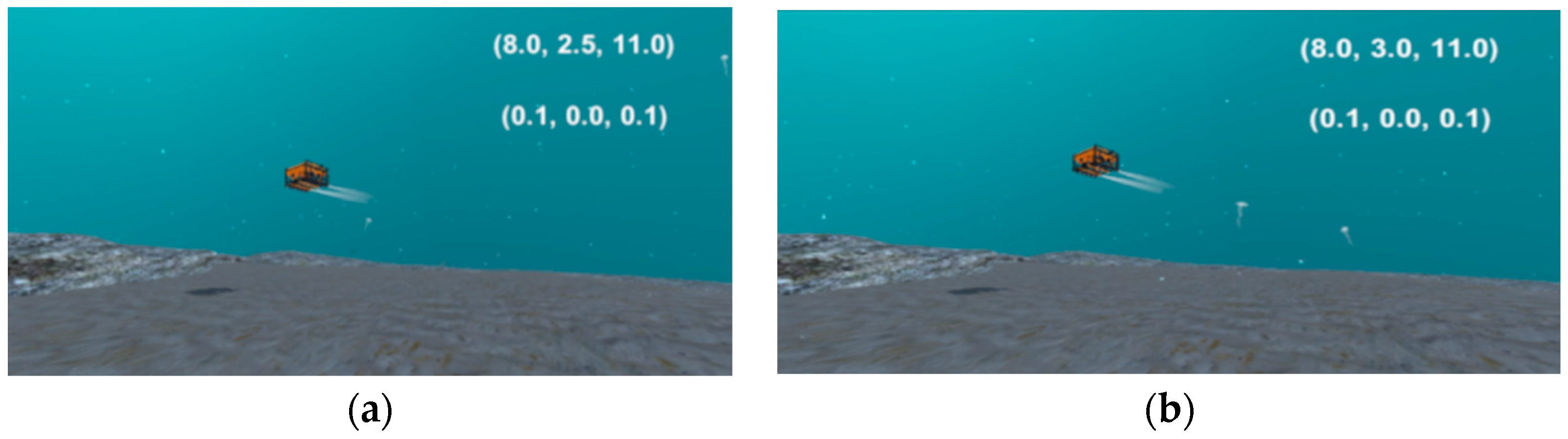
Different depth target values were set in the same way to conduct multiple sets of tests. This paper selected two sets of test results with depth target values of 2.5 m and 3.0 m, and the stability time was 14.6 s and 17.7 s, respectively, with an error of less than 0.1 m. As shown in Figure 19 below, it can be seen that the test results of multiple sets of depth setting simulations also met the control requirements.

Through the above tests, it was verified that the control effect of the algorithm meets the actual control requirements in the 3D simulation environment.

6. Pool Experiment

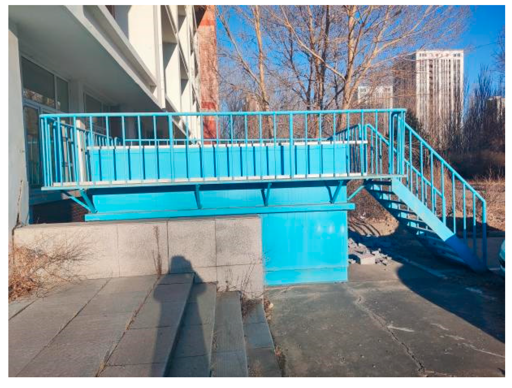
6.1. Experimental Environment

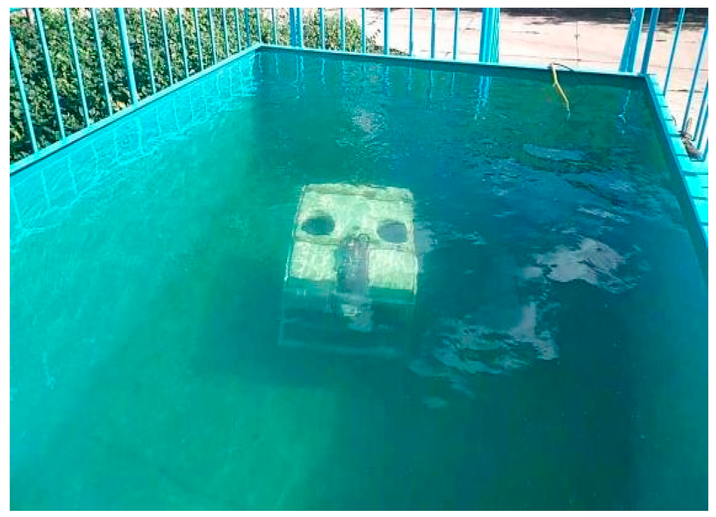
The environment of the underwater experiment was a water tank manufactured by the laboratory itself, with a length of 5 m, a width of 1.5 m, and a height of 2.2 m, which meets a series of experimental requirements such as depth setting and bow setting of the underwater robot, as shown in Figure 20.

6.2. ROV Depth Test

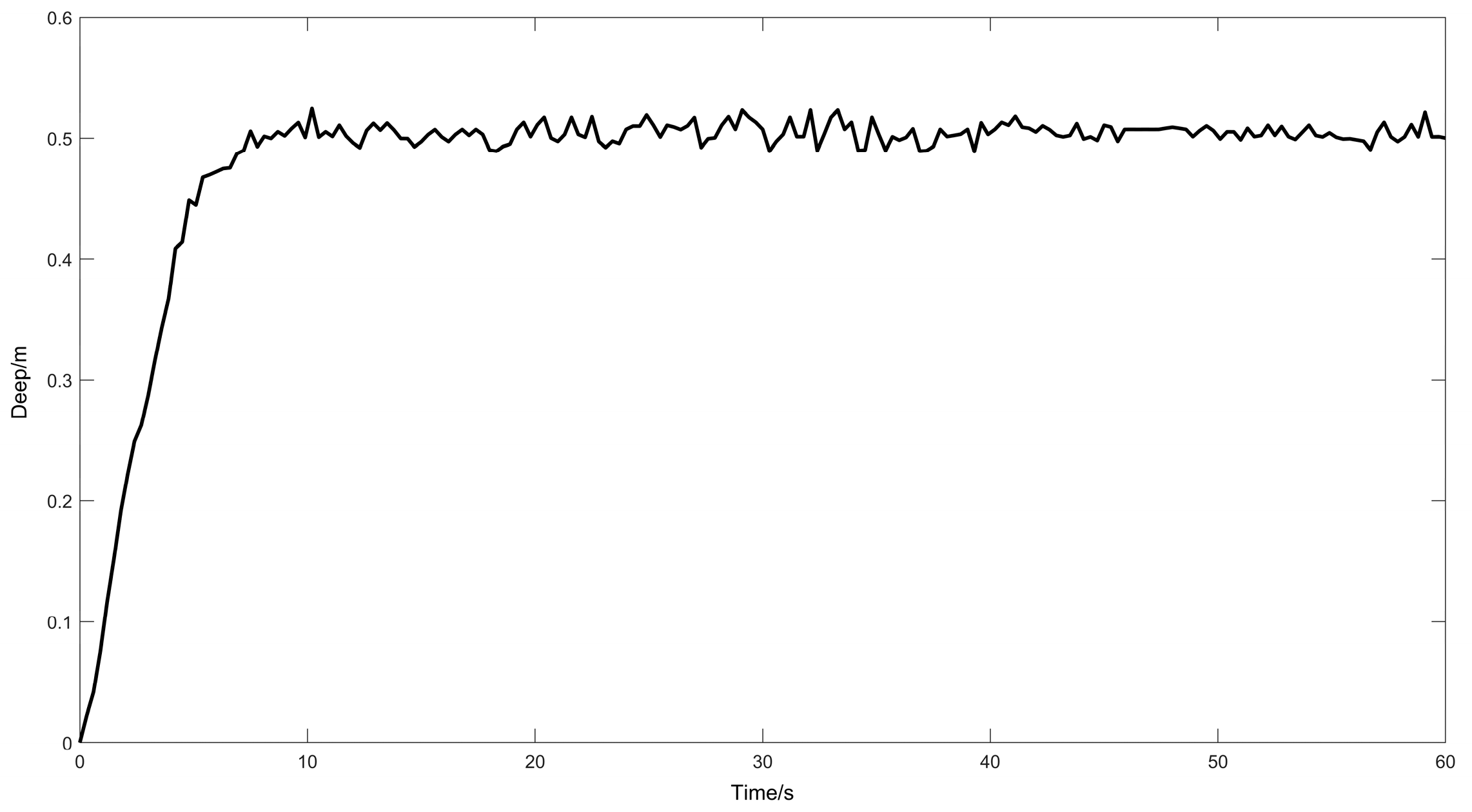
After the ROV was stabilized in the water, its initial depth was 0 m, and the target depth was set at 0.5 m. We observed the change of depth value from the upper computer monitoring interface and exported the data to record. Within 60 s, the software automatically recorded the depth value every 0.1 s, as shown in Figure 21.

The experimental data were sorted out and analyzed, and the curve image was drawn with MATLAB, as shown in Figure 22. In the fixed-depth experiment, the ROV stabilized after 9 s of adjustment time system and was able to maintain the target position well after stabilization, and its error was within the range of ±0.025 m. The experiment proves that the ROV depth-determination function has a good control effect and meets the design and operation requirements.

6.3. ROV Heading Test

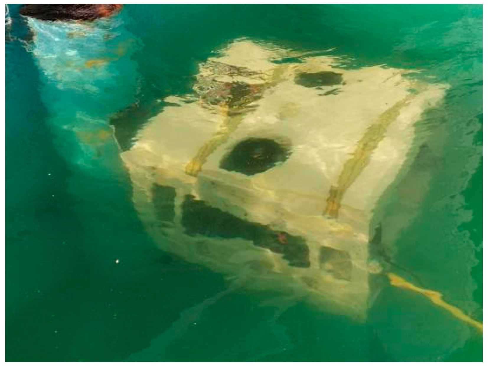
Next, we adjusted the initial heading angle of the ROV to 0°, set the target heading angle to 45°, and observed the change of the heading angle from the monitoring interface of the upper computer. The experiment process is shown in Figure 23. The experimental data were recorded and analyzed in the same way.

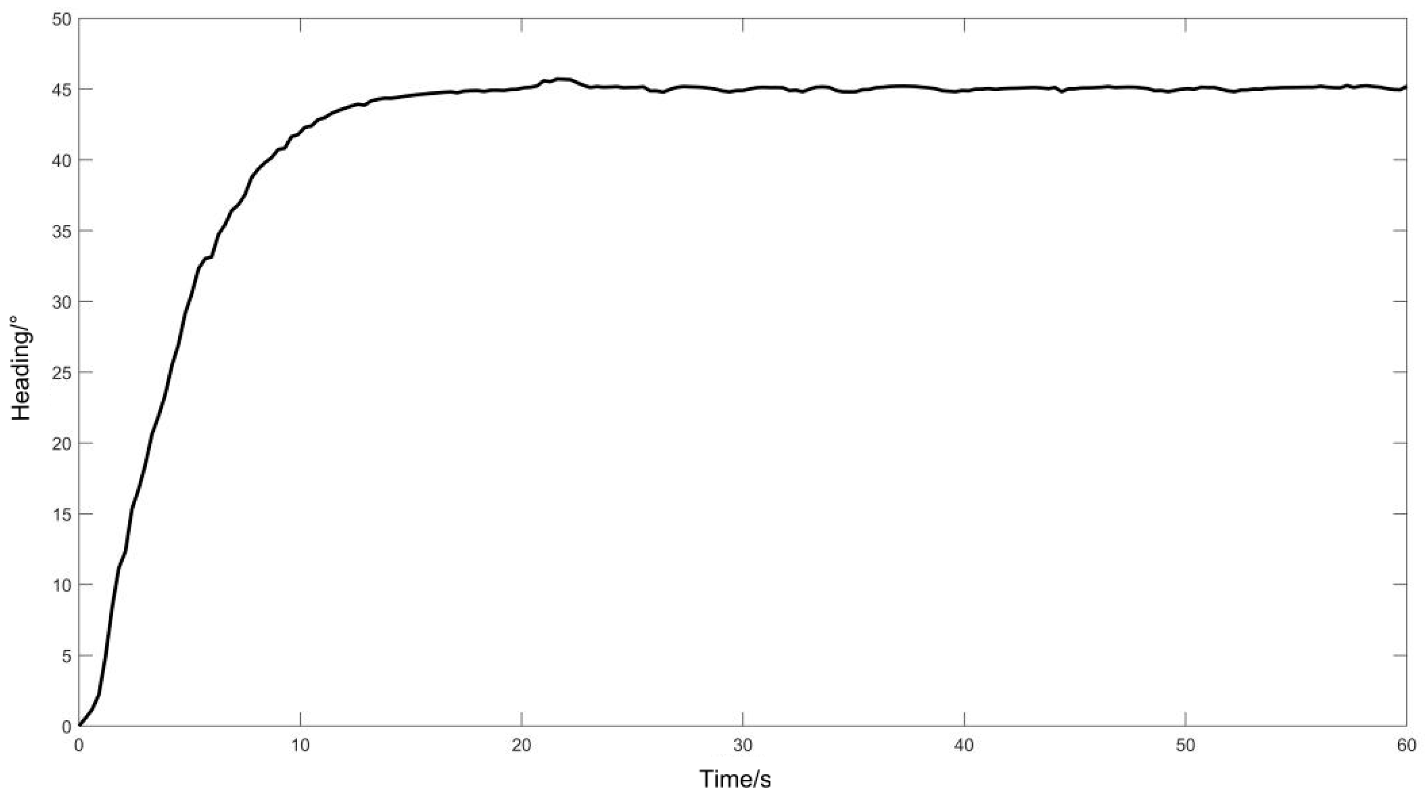
The ROV heading function data curve is shown in Figure 24. In the bow setting experiment, the ROV made the system enter a stable state after 15 s of adjustment time. After stabilization, the ROV could maintain the target heading well, and its error was within the range of ±2°. It is proven by the experiments that the control effect of the ROV’s bow positioning function is good, which meets the requirements of design and operation.

7. Conclusions

In this paper, a sliding mode control method based on saturation function is proposed for a six-degree-of-freedom ROV, which mainly solves the jitter problem in the classical sliding mode control and establishes a three-dimensional simulation system of Unity3D. Through the simulation experiment of classical PID, fuzzy PID, and the sliding mode controller designed in this paper and the pool experiment, the sliding mode control method demonstrated certain advantages. In the follow-up research, the research of multi-sensor data fusion will be further strengthened, aiming at the uncertainty of the ROV model; additionally, the parameters of the controller will be adjusted dynamically through adaptive changes to adapt to the uncertainty and changing working conditions.

References

- Dalhatu, A.; Azevedo, R.; Udebhulu, O. Recent developments of remotely operated vehicle in the oil and gas industry. Holos 2021, 3, 1–18. [Google Scholar]
- Mazzeo, A.; Aguzzi, J.; Calisti, M.L. Marine robotics for deep-sea specimen collection: A systematic review of underwater grippers. Sensors 2022, 22, 648. [Google Scholar] [CrossRef] [PubMed]
- Talkington, H. History and Accomplishments in Ocean Engineering at the Naval Ocean Systems Center, 1966–1983. In Proceedings of the OCEANS’83, San Francisco, CA, USA, 29 August–1 September 1983; IEEE: Piscataway, NJ, USA, 1983; pp. 384–387. [Google Scholar]
- Ratmeyer, V.; Rigaud, V. Europe’s growing fleet of scientific deepwater ROVs: Emerging demands for interchange, workflow enhancement and training. In Proceedings of the OCEANS 2009-EUROPE, Bremen, Germany, 11–14 May 2009; IEEE: Piscataway, NJ, USA, 2009; pp. 1–6. [Google Scholar]
- Odetti, A.; Bibuli, M.; Bruzzone, G. e-URoPe: A reconfgurable AUV/ROV for man-robot underwater cooperation. IFAC-PapersOnLine 2017, 50, 11203–11208. [Google Scholar] [CrossRef]
- Khatib, O.; Yeh, X.; Brantner, G. Ocean one: A robotic avatar for oceanic discovery. IEEE Robot. Autom. Mag. 2016, 23, 20–29. [Google Scholar] [CrossRef]
- Brantner, G.; Khatib, O. Controlling Ocean One: Human–robot collaboration for deep-sea manipulation. J. Field Robot. 2021, 38, 28–51. [Google Scholar] [CrossRef]
- Soylu, S. A chattering-free sliding-mode controller for underwater vehicles with fault-tolerant infinity-norm thrust allocation. Ocean Eng. 2008, 35, 1647–1659. [Google Scholar] [CrossRef]
- Huang, B.; Yang, Q. Double-loop sliding mode controller with a novel switching term for the trajectory tracking of work class ROVs. Ocean Eng. 2019, 178, 80–94. [Google Scholar] [CrossRef]
- Fossen, T. Nonlinear Modeling and Control of Underwater Vehicles; Norwegian Institute of Technology: Trondheim, Norway, 1991. [Google Scholar]
- Long, C.; Qin, X.; Bian, Y. Trajectory tracking control of ROVs considering external disturbances and measurement noises using ESKF-based MPC. Ocean Eng. 2021, 241, 109991. [Google Scholar] [CrossRef]
- Wu, X. Attitude stabilization control of autonomous underwater vehicle based on decoupling algorithm and PSO-ADRC. Front. Bioeng. Biotechnol. 2022, 10, 843020. [Google Scholar] [CrossRef] [PubMed]
- Wang, B. A low cost compact control system for the Hippo ROV. In Applied Mechanics and Materials; Trans Tech Publications Ltd.: Stäfa, Switzerland, 2012; Volume 190, pp. 627–633. [Google Scholar]
- Xu, S.; Ma, Q. Experimental study on inertial hydrodynamic behaviors of a complex remotely operated vehicle. Eur. J. Mech.-B/Fluids 2017, 65, 1–9. [Google Scholar] [CrossRef]
- Gabl, R.; Davey, T. Hydrodynamic loads on a restrained ROV under waves and current. Ocean Eng. 2021, 234, 109279. [Google Scholar] [CrossRef]
- Morinaga, A.; Yamamoto, I. Trajectory Planning Strategies and Simulation for Autonomous-surface-vehicle–Remotely-operated-vehicle (ASV–ROV) Cooperative System. Sens. Mater. 2023, 35, 411–422. [Google Scholar] [CrossRef]
- Shen, C.; Shi, Y.; Buckham, B. Path-following control of an AUV using multi-objective model predictive control. In Proceedings of the 2016 American Control Conference (ACC), Boston, MA, USA, 6–8 July 2016; IEEE: Piscataway, NJ, USA, 2016; pp. 4507–4512. [Google Scholar]
- Garcia-Valdovinos, L.; Fonseca-Navarro, F.; Aizpuru-Zinkunegi, J. Neuro-Sliding Control for Underwater ROV’s Subject to Unknown Disturbances. Sensors 2019, 19, 2943. [Google Scholar] [CrossRef] [PubMed]
- Wang, Z.; Liu, Y.; Guan, Z. An adaptive sliding mode motion control method of remote operated vehicle. IEEE Access 2021, 9, 22447–22454. [Google Scholar] [CrossRef]
- von Benzon, M. Integral Sliding Mode control for a marine growth removing ROV with water jet disturbance. In Proceedings of the 2021 European Control Conference (ECC), Rotterdam, The Netherlands, 29 June–2 July 2021; IEEE: Piscataway, NJ, USA, 2021; pp. 2265–2270. [Google Scholar]
- Sabau, A. Thrust force evaluation for a ROV (Remont Operating Vehicle) propeller. In Proceedings of the IOP Conference Series: Materials Science and Engineering, Iasi, Romania, 23–27 June 2020; IOP Publishing: Bristol, UK, 2020; Volume 916, p. 012098. [Google Scholar]
- Chin, C.; Lau, M. Design of thrusters configuration and thrust allocation control for a remotely operated vehicle. In Proceedings of the 2006 IEEE Conference on Robotics, Automation and Mechatronics, Bangkok, Thailand, 7–9 June 2006; IEEE: Piscataway, NJ, USA, 2006; pp. 1–6. [Google Scholar]
- Zohedi, F.; Aras, M. Comparison analysis of the PID controller and fuzzy logic controller (FLC) for a newly developed remotely operated vehicle (ROV) depth control. Proc. Mech. Eng. Res. Day 2020, 2020, 131–133. [Google Scholar]
- Xiang, X. Survey on fuzzy-logic-based guidance and control of marine surface vehicles and underwater vehicles. Int. J. Fuzzy Syst. 2018, 20, 572–586. [Google Scholar] [CrossRef]
- Chin, C. Unity3D serious game engine for high fidelity virtual reality training of remotely-operated vehicle pilot. In Proceedings of the 2018 10th international Conference on Modelling, identification and Control (iCMiC), Guiyang, China, 2–4 July 2018; IEEE: Piscataway, NJ, USA, 2018; pp. 1–6. [Google Scholar]
Figure 1.
Schematic diagram of ROV coordinate system.
Figure 2.
Original ROV model.
Figure 3.
Simplified ROV model.
Figure 4.
Direct motion simulation fluid domain.
Figure 5.
Rotary simulation fluid domain.
Figure 6.
Meshing of the direct moving fluid domain.
Figure 7.
Meshing of the rotating fluid domain.
Figure 8.
Schematic diagram of saturation function.
Figure 9.
Simulation model of sliding mode control.
Figure 10.
Classic PID simulation model.
Figure 11.
Fuzzy PID simulation model.
Figure 12.
Simulation diagram of snorkeling movement with fixed target value.
Figure 13.
Simulation diagram of snorkeling movement with changing target value.
Figure 14.
Simulation diagram of heading motion with fixed target value.
Figure 15.
Simulation diagram of heading motion with changing target value.
Figure 16.
Test effect with target angle of 90°. (a) Changes during heading motion test and (b) after heading motion test stabilization.
Figure 17.
Multi-group target angle test effect. (a) Test effect with target angle of 30°. (b) Test effect with target angle of 60°.
Figure 18.
Test effect with target depth of 2.0 m. (a) Changes during the depth test and (b) after the depth test was stabilized.
Figure 19.
Multi-group depth target test effect. (a) Test effect with target depth of 2.5 m. (b) Test effect with target depth of 3.0 m.
Figure 20.
Experimental water tank.
Figure 21.
Fixed-depth experiment diagram.
Figure 22.
Experimental data of fixed depth.
Figure 23.
Heading test diagram.
Figure 24.
Heading test data.