A Model Based on the Random Forest Algorithm That Predicts the Total Oil–Water Two-Phase Flow Rate in Horizontal Shale Oil Wells

Abstract

Due to variables like wellbore deviation variation and flow rate, the local flow velocity in the output wellbore of horizontal shale oil wells varied significantly at various points in the wellbore cross-section, making it challenging to calculate the total single-layer production with accuracy. The oil–water two-phase flow rate calculation techniques for horizontal wells developed based on particular flow patterns and array spinners had excellent applicability in their respective niches but suffered from poor generalizability and demanding experience levels for logging interpreters. In this study, we employed five spinners in a triangular walled array instrument to create the multi-decision tree after figuring out how many leaf nodes there were and examining the defining characteristics of the observed values gathered under various experimental setups. The construction of the entire oil–water two-phase flow prediction model was made possible when the random forest regression approach was used with it. The total oil–water flow rate at each perforated layer was predicted using the model in sample wells, and the mean square error with the third party’s interpretation conclusion was 1.42, indicating that the model had an excellent application effect. The approach, which offered a new interpretation method for calculating the oil–water two-phase flow rate of horizontal wells based on multi-location local flow rate, required less interpretation knowledge from the interpreter and had a stronger generalization capacity.

1. Introduction

Chinese continental shale oil has an enormous amount of potential for development [1,2,3]. Because of its multiple thin layers, the horizontal well volume fracturing exploitation method is commonly utilized [4,5,6]. Due to the early application of broad water injection techniques to enhance the recovery ratio, many existing wells were already enduring substantial water cut [7]. Conduct output profile logging is used to identify the high-producing water layer in order to plug water and boost production. Stratified flow and scattered flow are the two primary two-phase oil and water flow types in near horizontal wells. The distribution condition of oil and water in the wellbore fluctuated significantly due to variations in well trajectory, gravity’s effect, and flow rate near different production layers [8]. As a result, the water holdup distribution and velocity distribution are complex and varied. Traditional single-probe logging instruments with centered measurements did not accurately depict the fluid flow state in the wellbore. As a result, array capacitance, array resistance, and array fiber are frequently used to measure local holdup, while array spinner is frequently used to measure local velocity. These methods more correctly reflect the local flow information in the wellbore [9,10,11,12,13]. For total oil–water flow rate and fractional phase flow rate inversion calculations, among other things, stratified flow models and drift models are frequently created [14,15,16]. These explanatory models, however, typically only apply to particular flow types and have weak generalizability.

Wellbore deviation and fluid viscosity can cause different measurement deviations at different locations, which may affect the spinner response, increasing errors in flow rate interpretation and complicating logging interpretation. Local flow velocity measurements at various locations using various spinners are also influenced by these factors. The correct spinner response coefficients (slopes) and start-up speeds (the minimum fluid flow rate necessary for the spinner to start rotating) must be chosen for the interpretation in order to calculate accurate results when the fluid flow rate is calculated using conventional methods because various factors affecting the spinner response need to be compensated and corrected to ensure the accuracy and reliability of the interpretation model. The selection of slope, however, necessitated expert logging interpretation skills and was frequently prone to error. Currently, machine learning methods were frequently used to understand exploration log data [17,18,19,20] and production log output profiles [21]. As a form of machine learning technique, random forests provide predictions by constructing several decision trees. To lower the risk of overfitting and to increase the accuracy and stability of prediction, each decision tree is constructed using randomly chosen training data and features. Using distinct decision trees, the random forest algorithm learns and generates predictions individually before combining the output of many decision trees. This method is highly suited for handling challenging traffic prediction problems since it handles high-dimensional information and nonlinear interactions with effectiveness. In order to avoid the issue that the traditional production logging interpretation may be affected by a number of factors, which results in an inadequate generalization ability of the prediction, this paper attempts to use the random forest algorithm to predict the total oil–water two-phase flow rate of horizontal wells. It improves the universality of the interpretation approach and lessens the difficulty of production logging interpretation.

In this study, a multi-location array spinner instrument was used for data acquisition, and the experimentally gathered data points were used as training and test data to analyze the significance of each parameter, determine the number of decision trees and the number of leaf nodes, and finally establish an accurate predictive model of oil–water two-phase flow total flow rate in horizontal wells based on the random forest regression algorithm, which has high predictive ability and is widely used in practice.

2. Data Analysis

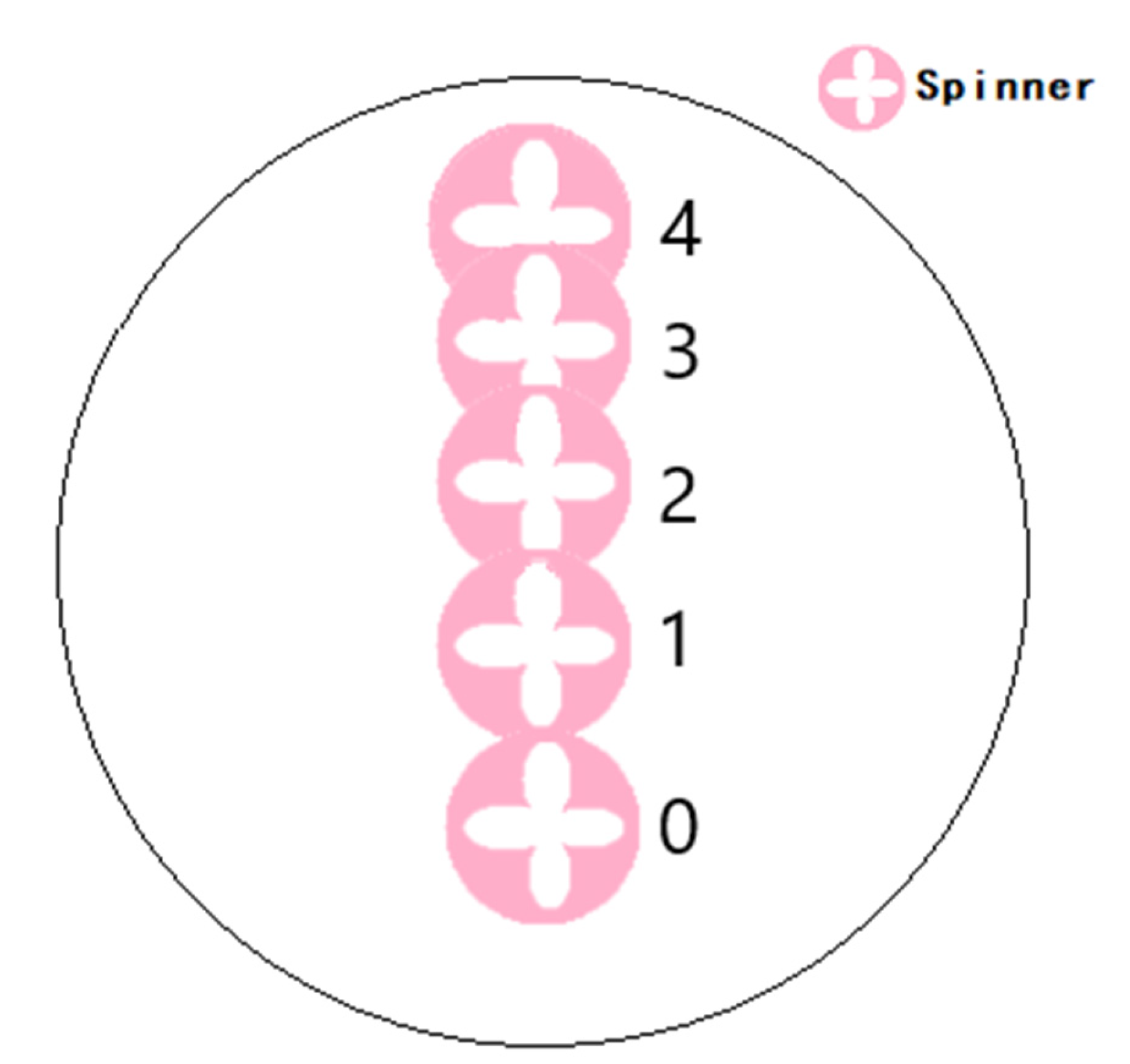
2.1. Experimental Setup

In this study, the diameter of the wellbore utilized in the experiment was 124 mm, and experiments were performed using a flow loop simulation device under various conditions of wellbore deviation of 85° and 90°, flow rates of 30, 40, and 50 m³/d, and water cut of 50, 70, and 90%. The array instrument employed in this study is shaped like a triangle arm with five spinners; the distribution of the spinners is shown in Figure 1. It can effectively cover the wellbore’s cross-section and gather data on the flow velocity of the entire borehole.

The flow rate at a single borehole cross-section was usually calculated when calculating the flow rate in the borehole, which led to the calculation of the flow rate for the entire borehole. Figure 2 depicts how the spinner is distributed across the wellbore cross-section.

The height of each spinner at the wellbore cross-section is calculated as in Equation (1).

$$y_i^{\prime }=CAL/2-\left(CAL/2-y_i\right)\times cosRO{T}_i$$

(1)

where $i$ is 0, 1, 2, 3, 4. $y_i^{\prime }$ is the height of the $i$th turbine after rotation, mm. $CAL$ is the diameter of the well, mm. $y_i$ is the height of the $i$th spinner caused by the instrumental process, mm. $RO{T}_i$ is the rotation angle of the $i$th probe, °.

2.2. Local Flow Velocity Calculation Method

The flow rates of the oil and water phases in horizontal wells differed as a result of the different densities of the oil and water phases. In order to calculate flow rate, three variables must be measured: flow velocity, time, and area. The rotating speed of the spinner can be transformed into the actual flow velocity of the fluid over a given length of time, representing the magnitude of the overall flow rate in the wellbore. A crucial sign for determining the flow rate in the wellbore visually is the spinner’s rotating speed in terms of magnitude. Similar to the relationship between windmill rotational speed and wind speed, there is a relationship between turbine rotational speed and flow rate. The turbine’s rotating speed rises in lock step with the wellbore fluid flow rate, much like a windmill does in the face of heavy winds. With this knowledge, we move on to start translating spinner RPM to fluid flow rate.

The calculation of the spinner speed and spinner local flow rate is calculated as Equation (2).

$$V_i=SPI{F}_i/K_i-SPEED+V_{thi}$$

(2)

where $V_i$ is the ith spinner’s calculated local flow velocity, m/min. $SPI{F}_i$ is the ith spinner’s response value, rps. $K_i$ is an experimentally calibrated coefficient, dimensionless. $SPEED$ is the cable’s speed, m/min. $V_{thi}$ is the experimentally calibrated start-up velocity of the $i$th spinner, m/min.

The relationship between the fluid flow velocity and spinner speed is a straight line through the origin in the ideal situation. However, when the fluid flow velocity is low, the mechanical friction and fluid viscosity cause the relation between the spinner speed and fluid flow rate to be curved, deviating from the straight line of the ideal condition. The influence of the mechanical friction decreases dramatically as the fluid flow rate rises; however, the main influencing element of the fluid viscosity causes the fitted straight line of the spinner speed and fluid flow rate to deviate slightly from the straight line in the ideal state [22]. Due to the influence of the mechanical friction and fluid viscosity, the fitted straight line and the ideal state of the fitted straight line of the offset are the spinner start-up speed $V_{th}$.

The cross plot of the cable speed and spinner speed can be used to calculate the spinner response coefficient (K), which is dictated by the manufacturing process. In the cable speed-turbine speed cross plot, the slope of the straight line fitted through the data points is then the spinner response coefficient K, and the intercept of the straight line with the horizontal axis is the minimum fluid flow velocity required for the spinner to start rotating, $V_{th}$. The spinner response coefficient of the same spinner differs slightly in the real application process due to variations in temperature, pressure, fluid characteristics, production conditions, etc. The full-flow layer and zero-flow layer must be used as the calibration layers in the actual logging interpretation process in order to draw a rendezvous diagram between the cable speed and the spinner speed and then calculate the spinner response coefficient (K) and start-up speed ($V_{th}$). Calibration layer selection and calculating the spinner response coefficient (K) are both qualitative processes that depend on the interpreter’s previous experience. A cross plot of the spinner 0 response data and cable speed for three full-flow and three zero-flow layers chosen for a specific application is displayed in Figure 3.

“Full-Flow Layer” is Full-Flow Layer, and “Zero-Flow Layer” is Zero-Flow Layer, as seen in the Figure 3. “DN” stands for Downward Pull Measurement, and the cable speed is positive. “UP” stands for Upward Pull Measurement, and the cable speed is negative. “SPIF0” is the 0th spinner’s response value. $“SPEED”$ is the cable’s speed. The spinner response coefficient (K) is the average of the slopes of the fitted straight lines for the downward pull measurement and the upward pull measurement in the same scale layer in the cross plot of the cable speed and spinner speed. The intercept on the horizontal axis of the fitted straight line for measurements of downward pull and upward pull in the same calibration layer is averaged to obtain the start-up speed of the spinner, $V_{th}$.

At this stage, a decision is required to select the suitable result because the spinner response coefficient (K) and start-up speed ($V_{th}$) fitted by the cross plot are different for the different calibration layers. As a result, there is uncertainty and potential for error in the calculation of the spinner response coefficient (K) and startup speed ($V_{th}$).

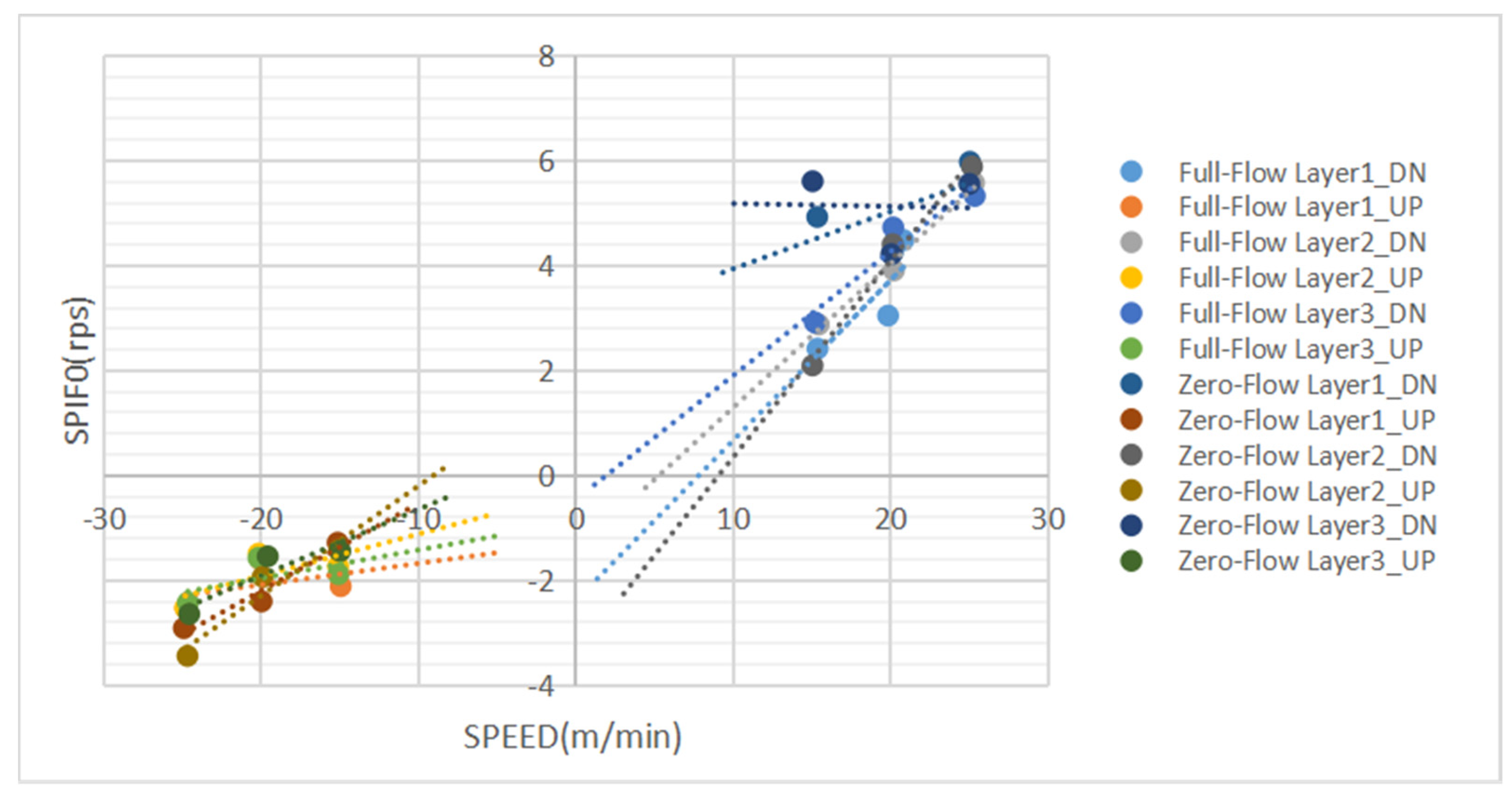
2.3. Analysis of Flow Velocity Influencing Factors

Equation (1) is used to compute the local flow velocity of each spinner after determining its response coefficient (K) and start-up velocity ($V_{th}$). The flow velocity curve of the wellbore cross-section is fitted by the local flow velocity of each spinner using the quartic polynomial. The fitting procedure is as follows: a quadratic polynomial fitting function is used to eventually fit the local flow velocity profiles at various heights throughout the wellbore cross-section, using the height $y_i^{\prime }$ of the five turbines on the wellbore as the dependent variable and the local flow velocity $V_i$ as the independent variable.

Next, the integral is used to calculate the average flow velocity on the wellbore cross-section. Finally, the total flow rate of the horizontal well is calculated. The flow velocity curve in the wellbore cross-section is affected by the cable speed and wellbore deviation as shown in Figure 4. As shown in Figure 4, where the horizontal axis is the fluid flow velocity and the vertical axis is the height of the wellbore section, “DEV” is deviation, and stands for wellbore deviation, “CW” stands for water cut, “QT” stands for total oil–water flow rate and “SPEED” for the cable speed. The values of the vertical axis coordinates of the red hollow dots correspond to the height of the spinner in the wellbore cross-section in the experimental photographs.

The area filled by the oil and water phases is comparable at a wellbore deviation of 90° with 50% water cut, as shown in Figure 4. The lighter mass oil phase has a larger flow velocity when the wellbore deviation is 85°, and the local flow velocity is greatest at the height where spinner 4 is situated. The fitted curves demonstrate that the local flow velocities at the heights of spinner 1 and spinner 4 are similar when the wellbore deviation is 90° and the cable speed is lower. The flow velocity of the oil phase is greater than the flow velocity of the water phase in the whole wellbore cross-section as the absolute value of the cable speed rises, meaning that the local flow velocity at the height where spinner 4 is positioned is greater than that at the height where spinner 1 is located.

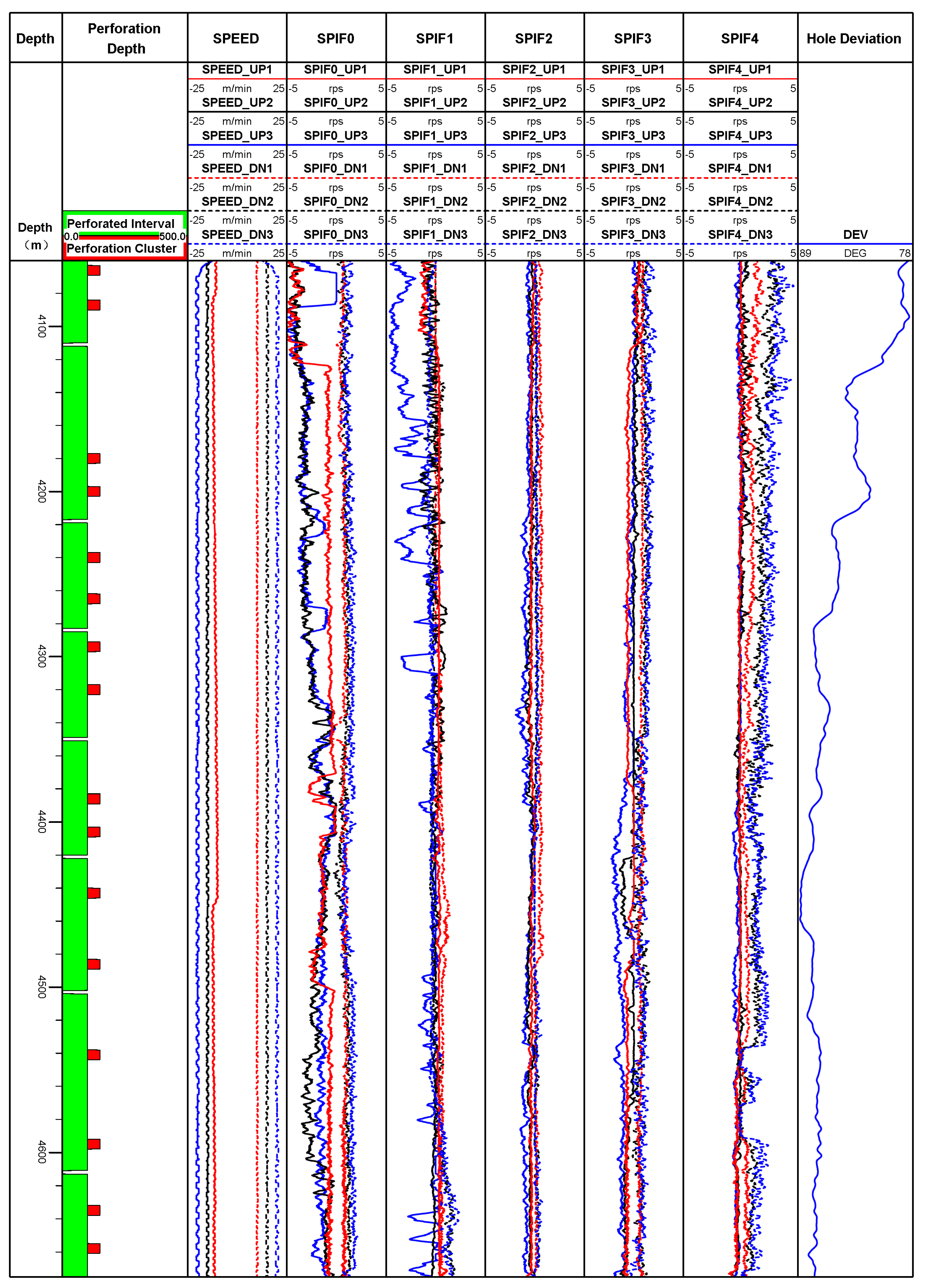
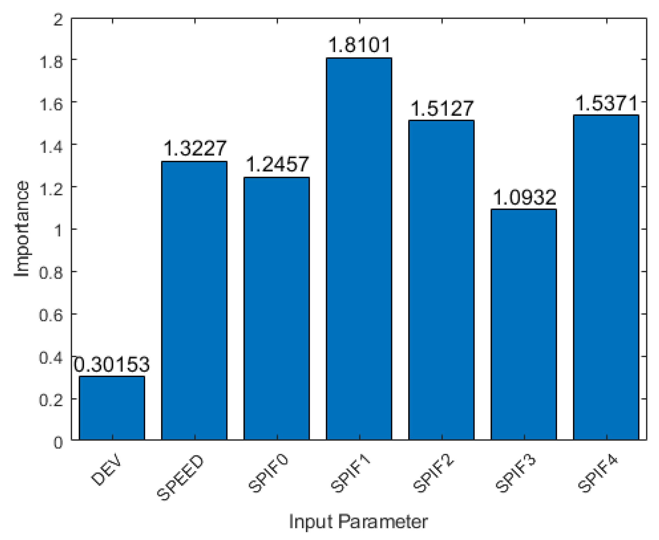
2.4. Characteristic Parameter Analysis

It is known from the previous section that several variables, including the cable speed, turbine response value, and well slope, have an impact on the calculation of the overall flow rate of horizontal wells. In order to create the flow rate prediction model based on the random forest regression technique, the data for the wellbore deviation, the cable speed, and the five spinners response values are employed as input characteristic parameters. The raw data must be cleaned and processed, and any potential outliers must be identified and dealt with in order to assure the consistency and dependability of the data. To ensure that the input characteristics are complete, missing value data are filled in if they exist in the data. Outliers are also removed in order to avoid interfering with the model’s training and prediction.

Table 1. Characteristic parameters for predicting oil–water two-phase flow total flow rate in.

Characteristic Parameter	Range	Mean Value	Standard Deviation
SPEED (m/min)	−21.18~−10.18	−17.73	2.64
SPIF0 (rps)	−7.44~−0.41	−3.24	1.01
SPIF1 (rps)	−7.52~0.42	−4.47	1.76
SPIF2 (rps)	−9.02~−1.47	−4.93	1.53
SPIF3 (rps)	−8.53~4.68	−3.92	1.23
SPIF4 (rps)	−5.64~1.67	0.22	1.38
DEV (°)	85~90	88.21	2.40

displays the characteristics of the input parameter. In the table, “SPEED” is the cable speed, “SPIF” is the spinner response value, and “DEV” is the wellbore deviation. The training set was drawn from a randomly chosen 70% of the dataset, while the test set was drawn from the remaining 30%.

The interpretability of the random forest algorithm is primarily due to its capacity to assess the significance of each input variable and determine the extent to which each input parameter influences the prediction outputs. The process of determining importance typically involves first categorizing the input parameters, then choosing the best features for node splitting by comparing their Gini coefficients before and after splitting, and finally determining the extent to which feature splitting improved the model by using the Out-of-Bag (OOB) error to determine the relative importance of each feature.

The Gini coefficient is calculated as in Equation (3).

$$G=1-{{\displaystyle \sum }}_{i-1}^C{\left(P_i\right)}^2$$

(3)

where C is the number of categories. $P_i$ is the proportion of samples belonging to category $i$ in this node.

For each sample $i$ in the random forest, assuming that there are $T$ trees in the random forest model and sample $i$ is not sampled in the $t$th tree (which is an OOB sample), its prediction can be calculated as ${\widehat{y}}_l^t$. Its OOB error is calculated as in Equation (4).

$$O=1/T_i{{\displaystyle \sum }}_{t=1}^{T_i}L\left(y_i, {\widehat{y}}_l^t\right)$$

(4)

where $O$ denotes the OOB error for the sample $i$. $T_i$ denotes the number of times sample $i$ is in all tree photos as a sample. $L\left(y_i, {\widehat{y}}_l^t\right)$ is a loss function that measures the error between the predicted value ${\widehat{y}}_l^t$ and the true value $y_i$. For regression problems, the squared loss is usually used and is calculated as in Equation (5).

$$L\left(y_i, {\widehat{y}}_l^t\right)={\left(y_i-{\widehat{y}}_l^t\right)}^2$$

(5)

Figure 5 displays a histogram of the significance of each characteristic parameter on the flow rate forecast, which demonstrates that the important values for spinners 1 and 4 are higher, which is more in line with the pattern in Figure 3 overall. The calculation of the horizontal well’s total flow rate is influenced by the cable speed, spinner response value, and wellbore deviation.

3. Random Forest Algorithm and Model Construction

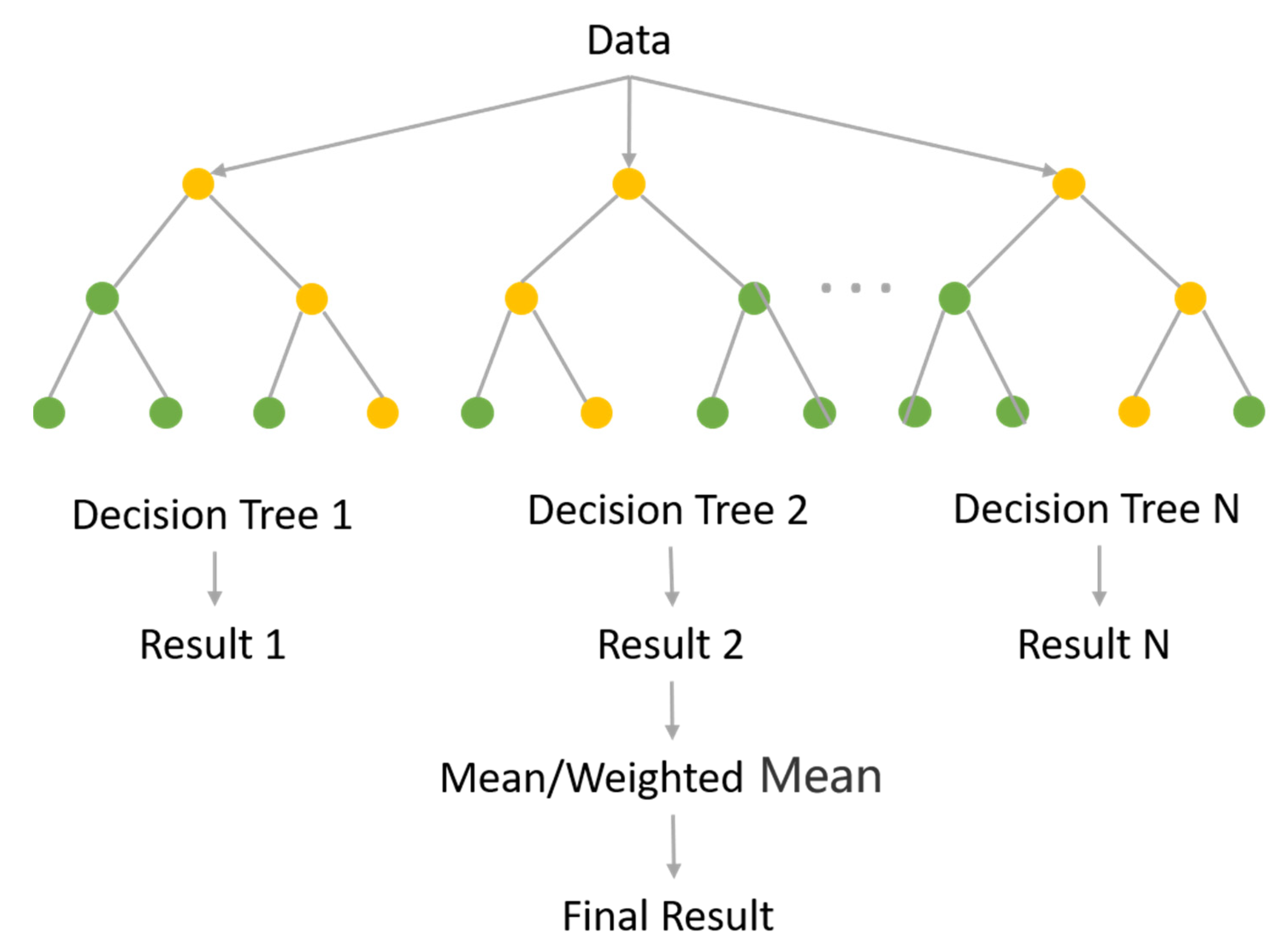
3.1. Principle of Random Forest Algorithm

In the area of machine learning, random forest belongs to the field of integrated learning. Its distinctive quality is that it creates a potent predictive model by constructing numerous separate decision trees. Each decision tree in random forest is created using a randomly chosen collection of features and training data. By introducing this randomness, the model’s accuracy and generalizability are improved as redundant features have less of an impact on the prediction outcomes. The sample data utilized in the random forest training process for constructing each decision tree are also collected by random sampling, further enhancing the model’s diversity. As each decision tree is trained using a different subset of features and data, they have a high degree of independence and are less likely to overfit. The construction procedure is as follows:

(1)

A finite number of samples may be drawn numerous times, and selecting is performed from the original dataset; the gathered samples are the same size as the original dataset.

(2)

Assume that M attribute features make up the sample and that m of those features is chosen at random for node splitting, with m being substantially smaller than M.

(3)

Use step (2) to continue splitting the selected nodes until a stopping condition is fulfilled. This stopping condition may be that the maximum depth of the decision tree has been reached or the number of samples in the node is below a threshold etc.

(4)

Keep repeating steps (2) and (3) to create a multitude of decision trees that eventually combine to form a random forest.

Depending on the tree’s initial data, each decision tree chooses the best splitting method. The decision tree outputs from each decision tree are ultimately averaged or weighted to provide the prediction results of the random forest. With less reliance on the initial data, this method produces more accurate predictions. Figure 6 displays the random forest’s schematic diagram.

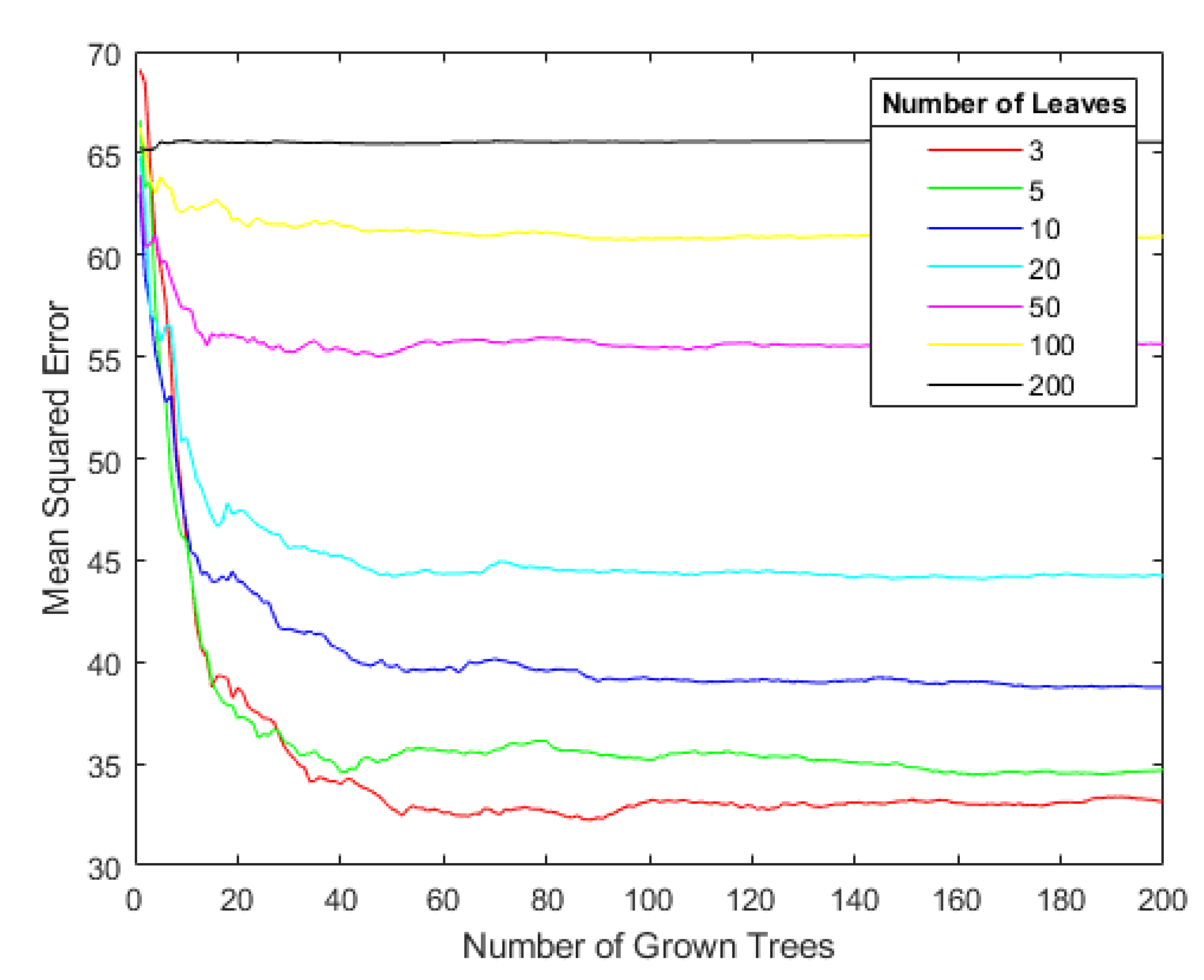
3.2. Model Construction

When creating a single decision tree, the importance of the input feature parameter was used to determine the probability that the feature parameter would be chosen at random as the next leaf node. Once the predetermined number of leaf nodes is reached, the split proceeds downward until the algorithm’s optimal decision tree depth is reached. The optimal number of leaf nodes and decision trees must be identified before building the oil–water two-phase flow total flow prediction model for horizontal wells based on the random forest regression algorithm. In this study, the performance of the model is tested by testing different numbers of leaf nodes, which are set to 3, 5, 10, 20, 100, and 200. The mean square error under different numbers of leaf nodes and decision trees is evaluated, and the mean square error is determined as in Equation (6). Figure 7 displays the mean square error for various leaf nodes and decision tree counts.

$$MSE=1/N\times \sum {\left(y-\widehat{y}\right)}^2$$

(6)

where $MSE$ denotes mean square error. $N$ denotes sample size. $y$ denotes true value. $\widehat{y}$ denotes predicted value.

Figure 7 shows that when the number of leaf nodes is set to 3, the mean square error drops to its lowest value. When there are roughly 60 decision trees, the mean square error of each curve no longer declines. Therefore, the choice is made to build the flow prediction model in this research using a combination of 3 leaf nodes and 60 decision trees.

A flow prediction model built on the random forest method can be created by setting the number of leaf nodes, the number of decision trees, and the regression technique. Use the existing flow prediction model to input the horizontal well logging data for the cable speed, response value, and wellbore deviation to calculate the total oil and water two-phase flow rate.

Figure 8 compares the actual flow rate for the experimental total oil–water flow test sets of 30, 40, and 50 m³/d to the model-predicted flow rate. The training set’s test data, which were acquired by randomly selecting 30% of the total sample data, are represented in the figure by the blue data points. The model’s predicted flow rate is represented by the horizontal coordinate in the graph, while the test data’s actual flow rate is represented by the vertical coordinate. The red solid line’s points indicate that predicted and actual flow rates are equal. The 10% error line between a predicted flow rate and the actual flow rate is represented by the red dashed line. From the figure, it can be seen that the prediction errors are essentially within the range of 10%, indicating that the prediction results of the model were relatively accurate. However, when the predicted flow rate is in error, the predicted flow rate is always greater than 30 m³/d when the true flow rate is 30 m³/d, while the predicted flow rate is always less than 50 m³/d when the true flow rate is 50 m³/d. This phenomenon occurs because the flow rate of the training data used to build the random forest model is between 30 and 50 m³/d, causing the model to have a tendency to converge the flow prediction results to the 30 to 50 m³/d interval during the prediction process.

In this paper, the performance of the developed model is evaluated using the mean square error and the coefficient of determination, which is calculated as follows.

$$SST=\sum {\left(y_i-\overline{y}\right)}^2$$

(7)

where $SST$ means the total variance of the sample. $y_i$ means the true value of the $i$ th sample. $\overline{y}$ means the mean of the true value of the sample.

$$SSE=\sum {\left(y_i-\widehat{y_l}\right)}^2$$

(8)

where $\mathit{SSE}$ means the sum of squared residuals. $y_i$ means the true value of the th sample. $\widehat{y_l}$ means the th model predicted value.

$$R^2=1-\left(SSE/SST\right)$$

(9)

where $R^2$ is the coefficient of determination of the model. $SSE$ denotes the sum of squared residuals. $SST$ denotes the total variance of the sample.

As shown in

Table 2. Table of error results.

Mean Squared Error	Decision Coefficient
2.77	0.95

, the model’s mean squared error, which is 2.77, represents a decent overall prediction performance. The model has a high degree of interpretability, as indicated by the coefficient of determination of 0.95. In conclusion, the model’s predicted flow rate shows good explanatory accuracy.

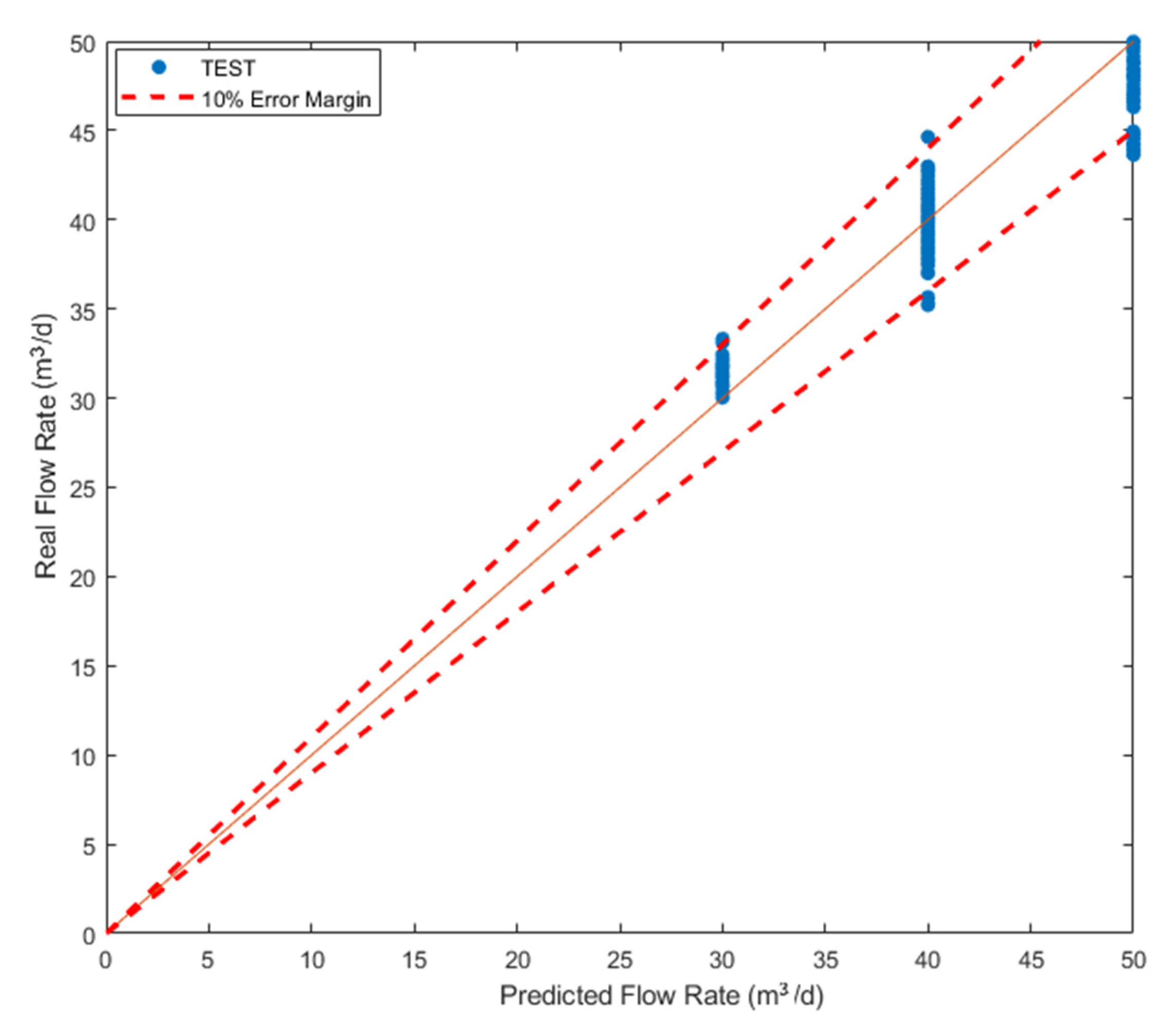
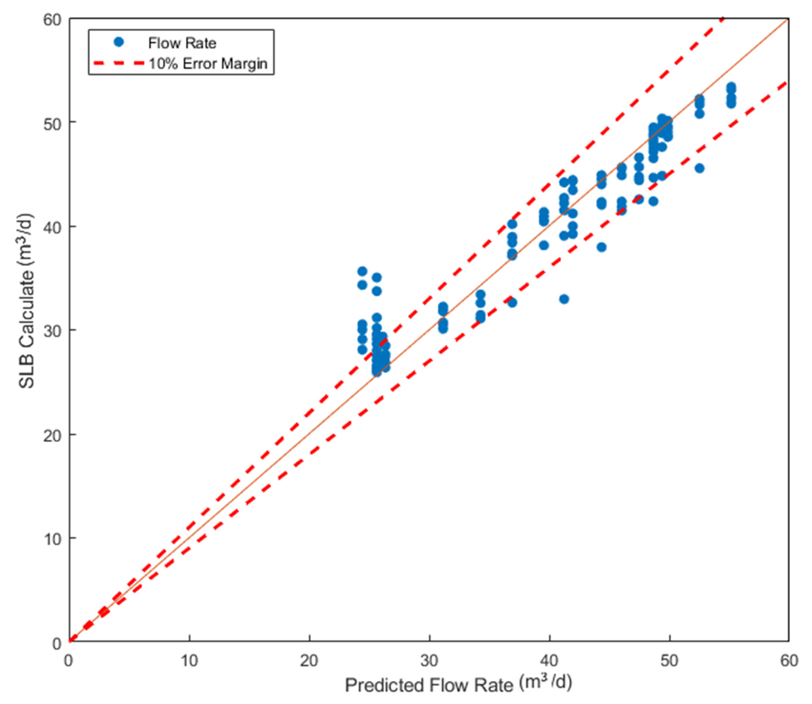
4. Example Verification

The horizontal shale oil well known as well A had eight perforation layers, sixteen perforation clusters, a wellbore deviation between 78 and 89 degrees, a total flow rate of 56 m³/d, and severe fluid accumulation in the wellbore with a water holdup of more than 90%. The cable pull measurement was used, and the measurement included three upward pull measurements and three downward pull measurements, for a total of six trips to measure the speed data, and the measurement data is shown in Figure 9.

A total of 132 sets of data were collected from values gathered close to the perforation cluster. In this study, the flow rate was forecasted using a flow rate prediction model based on the random forest regression technique. The flow rate results for well A were predicted using the cable speed, spinner response value, and wellbore deviation data. Schlumberger’s well logging interpretation findings are concluded by the interpreters’ interpretation expertise following a number of procedures like curve data quality control, spinner calibration, and interpretation technique selection. The mean square error between the flow rate results predicted in this paper and interpreted by Schlumberger is 1.42. A comparison of the flow rate is shown in Figure 10.

According to the model developed in this study, the horizontal coordinates in the image indicate the total oil–water two-phase flow rate at each layer of well A, whereas the vertical coordinates show Schlumberger’s interpretation results. The red dashed line represents the 10% error line, and the points on the red solid line show that the flow rate determined in this study matches Schlumberger’s flow rate interpretation results exactly. According to the graph, when the total flow is between 30 and 50 m³/d, both errors are often less than 10%, demonstrating the great accuracy and usefulness of the flow forecast model. However, a portion of the data has a higher inaccuracy when the flow rate is less than 30 m³/d.

5. Conclusions

Shale oil horizontal well output profile logging is influenced by a variety of circumstances, making the typical logs interpretation approach difficult, requiring highly skilled interpreters, and inadequately generalized. In this study, the oil–water two-phase flow total flow prediction model for horizontal wells was developed utilizing the random forest regression technique based on the measurements of the multi-position array spinner, cable speed measurement, and wellbore deviation data. Using experimental data, the model was tested, and the test mean square error is 2.77, with good overall prediction outcomes and accuracy of forecast. When the model was applied correctly to an example, the mean square error of the model’s predicted flow is 1.42, and the difference between Schlumberger’s interpretation and prediction results is essentially 10%, which is an excellent application result. The model performed better at flow rates between 30 and 50 m³/d, and the accuracy will be decreased in other flow rate ranges, as determined by the properties of the training data. As a result, the follow-up work should carry out more pertinent tests to enhance the model and boost forecast accuracy.

References

1. Zhao, W.; Bian, C.; Li, Y.; Zhang, J.; He, K.; Liu, W.; Zhang, B.; Lei, Z.; Liu, C.; Zhang, J.; et al. Enrichment factors of movable hydrocarbons in lacustrine shale oil and exploration potential of shale oil in Gulong sag, Songliao Basin, NE China. Pet. Explor. Dev. 2023, 50, 455–467. [Google Scholar] [CrossRef]
2. Yuan, S.; Lei, Z.; Li, J.; Yao, Z.; Li, B.; Wang, R.; Liu, Y.; Wang, Q. Key theoretical and technical issues and countermeasures for effective development of Gulong shale oil, Daqing Oilfield, NE China. Pet. Explor. Dev. 2023, 50, 638–650. [Google Scholar] [CrossRef]
3. Li, Y.; Zhao, Q.; Lyu, Q.; Xue, Z.; Cao, X.; Liu, Z. Evaluation technology and practice of continental shale oil development in China. Pet. Explor. Dev. 2022, 49, 1098–1109. [Google Scholar] [CrossRef]
4. Pang, X.; Li, M.; Li, B.; Wang, T.; Hui, S.; Liu, Y.; Liu, G.; Hu, T.; Xu, T.; Jiang, F.; et al. Main controlling factors and movability evaluation of continental shale oil. Earth-Sci. Rev. 2023, 243, 104472. [Google Scholar] [CrossRef]
5. Jin, X.; Li, G.X.; Meng, S.W.; Wang, X.Q.; Liu, C.; Tao, J.P.; Liu, H. Microscale comprehensive evaluation of continental shale oil recoverability. Pet. Explor. Dev. 2021, 48, 222–232. [Google Scholar] [CrossRef]
6. Zhou, X.Y.; Wei, M.X.; Zhang, Y.R.; Li, T.; Xu, S. Reservoir Benefit Classification and Development Countermeasures for Changqing Oilfield. Xinjiang Pet. Geol. 2022, 43, 320–323+340. [Google Scholar]
7. Cai, M. Current situation and prospect of main technology of oil production engineering in Daqing Oilfield. Oil Drill. Prod. Technol. 2022, 44, 546–555. [Google Scholar]
8. Liu, J.F.; Shi, S.B.; Chen, H. Experimental Research on Oil-Water Flow Imaging in Near-Horizontal Well Using Single-Probe Multi-Position Measurement Fluid Imager. Processes 2022, 10, 1051. [Google Scholar] [CrossRef]
9. Andreussi, P.; Pitton, E.; Ciandri, P.; Picciaia, D.; Vignali, A.; Margarone, M.; Scozzari, A. Measurement of liquid film distribution in near-horizontal pipes with an array of wire probes. Flow Meas. Instrum. 2016, 47, 71–82. [Google Scholar] [CrossRef]
10. Xu, L.; Zhang, W.; Zhao, J.; Cao, Z.; Xie, R.; Liu, X.; Hu, J. Support-vector-regression-based prediction of water holdup in horizontal oil-water flow by using a bicircular conductance probe array. Flow Meas. Instrum. 2017, 57, 64–72. [Google Scholar] [CrossRef]
11. Li, Q.Z.; Liu, J.F.; Gao, F.; Dai, Y.X.; Peng, W.S. Interpretation Method of Oil-Water Two-Phase Flow in Horizontal Well Based on Array Spinner and Array Holdup Tools. Well Logging Technol. 2021, 45, 405–410+430. [Google Scholar]
12. Liu, J.F.; Xu, Y.C.; Wu, Q.X. Holdup flow imaging analysis for capacitance and resistance ring array probes. Prog. Geophys. 2018, 33, 2141–2147. [Google Scholar]
13. Cui, S.F.; Liu, J.F.; Li, K. Data Analysis of Two-Phase Flow Simulation Experiment of Array Optical Fiber and Array Resistance Probe. Coatings 2021, 11, 1420. [Google Scholar] [CrossRef]
14. Cui, S.F.; Liu, J.F.; Chen, X.L. Experimental Analysis of Gas Holdup Measured by Gas Array Tool in Gas–Water Two Phase of Horizontal Well. Coatings 2021, 11, 343. [Google Scholar] [CrossRef]
15. Song, H.; Guo, H.; Guo, S.; Shi, H. Partial phase flow rate measurements for stratified oil-water flow in horizontal wells. Pet. Explor. Dev. 2020, 47, 613–622. [Google Scholar] [CrossRef]
16. Cui, S.F. Method of Horizontal Well Array Flow Image Research on Simulation Experiment and Interpretation. Master’s Thesis, Yangtze University, Wuhan, China, 2023. [Google Scholar]
17. Liang, H.; Liu, G.; Zou, J.; Bai, J.; Jiang, Y. Research on calculation model of bottom of the well pressure based on machine learning. Future Gener. Comput. Syst. 2021, 124, 80–90. [Google Scholar] [CrossRef]
18. Nwanwe, C.C.; Duru, U.I.; Anyadiegwu, C.; Ekejuba, A.I.B. An artificial neural network visible mathematical model for real-time prediction of multiphase flowing bottom-hole pressure in wellbores. Pet. Res. 2022, in press. [Google Scholar] [CrossRef]
19. Sami, N.A. Application of machine learning algorithms to predict tubing pressure in intermittent gas lift wells. Pet. Res. 2022, 7, 246–252. [Google Scholar] [CrossRef]
20. Liu, J.; Jiang, L.; Chen, Y.; Liu, Z.; Yuan, H.; Wen, Y. Study on prediction model of liquid hold up based on random forest algorithm. Chem. Eng. Sci. 2023, 268, 118383. [Google Scholar] [CrossRef]
21. Wahid, M.F.; Tafreshi, R.; Khan, Z.; Retnanto, A. Prediction of pressure gradient for oil-water flow: A comprehensive analysis on the performance of machine learning algorithms. J. Pet. Sci. Eng. 2022, 208, 109265. [Google Scholar] [CrossRef]
22. Guo, H.; Dai, J.; Chen, K. Production Logging Principles and Data Interpretation; Petroleum Industry Press: Beijing, China, 2007; pp. 35–37. [Google Scholar]
Figure 1. Schematic diagram of spinner distribution.
Processes 11 02346 g001
Figure 2. Schematic diagram of the spinner in the wellbore section.
Processes 11 02346 g002
Figure 3. Cable speed and spinner speed cross plot.
Processes 11 02346 g003
Figure 4. Wellbore cross-sectional flow velocity curve.
Processes 11 02346 g004
Figure 5. Histogram of the importance of feature parameters.
Processes 11 02346 g005
Figure 6. Schematic diagram of random forest principle.
Processes 11 02346 g006
Figure 7. Plot of mean square error with different leaf nodes and number of decision trees.
Processes 11 02346 g007
Figure 8. Comparison of test flow rate and predicted flow rate.
Processes 11 02346 g008
Figure 9. Measurement curve of well A.
Processes 11 02346 g009
Figure 10. Comparison of predicted flow rate of well A and calculated flow rate of SLB.
Processes 11 02346 g010