Abstract
Feature data refer to direct measurements of specific features, while feature residuals represent the deviations between these measurements and their corresponding benchmark values. Both types of information offer unique insights into the system’s behavior. However, conventional diagnostic systems often struggle to effectively integrate and utilize both types of information concurrently. To address this limitation and improve diagnostic performance, a hybrid method based on the Bayesian network (BN) is proposed. This method enables the parallel fusion of feature residuals and feature data within a unified diagnostic model, and a comprehensive framework for developing this hybrid method is also given. In the hybrid BN, the symptom layer consists of residual nodes representing feature residuals and data nodes representing measured feature data. By applying the proposed method to two chillers and comparing it with state-of-the-art existing methods, we demonstrate its effectiveness and superiority. The results highlight that the proposed method not only accommodates the absence of either type of information but also leverages both of them to enhance diagnostic performance. Compared to using a single type of node, the hybrid method achieves a maximum improvement of 24.5% in diagnostic accuracy, with significant enhancements in F-measure observed for refrigerant leakage fault (34.5%) and excessive lubricant fault (32.8%), respectively.
1. Introduction
Buildings play a critical role as the primary consumers of energy, accounting for around 40% of global energy consumption [1]. Among the energy-consuming systems in buildings, chillers are major contributors. However, when a chiller malfunctions, it can lead to reduced efficiency, energy waste, shortened lifespan, and compromised indoor comfort. In fact, a faulty chiller can result in an additional 30% increase in energy consumption [2]. Therefore, fault diagnosis plays a vital role in detecting and resolving issues with chillers, leading to significant energy savings.
After decades of development, fault diagnosis of chillers has been widely studied, and a large number of methods have been proposed and applied. Generally, these methods can be categorized into two types: model-driven and data-driven methods.
Model-driven methods usually establish a model that can identify and assess deviations (known as residuals) between actual operating levels and predefined normal (benchmark) operating levels. One of the main applications of model-driven methods is the acquisition of feature residuals. These residuals represent the differences between measured feature data and their corresponding benchmark values. The benchmark values are derived from a benchmark model and signify the system’s normal operating state. In the realm of model-based approaches, Browne and Bansal [3] summarized and analyzed the relevant literature on steady-state models of the chiller. Additionally, Zhao et al. [4] and Kim and Braun [5,6] developed fault diagnosis techniques based on simplified physical models and decoupling models, respectively.
Data-driven methods analyze a substantial amount of measured data related to specific features for each fault to extract patterns. These patterns are then utilized to diagnose faults by identifying similarities among them. Data-driven methods are particularly effective in utilizing feature data, which refers to directly measured data of features. In recent years, with the rapid advancements in computer technology and artificial intelligence, data-driven methods have gained significant popularity in the field of fault diagnosis [7]. Examples of such methods include support vector machine (SVM) [8], convolutional neural network (CNN) [9], global density-weighted support vector data description [10], association rule mining [11], and unsupervised clustering models such as K-means, Gaussian mixture model clustering, and spectral clustering [12], among others.
In recent years, there has been a growing interest among researchers in integrating multiple methods to enhance diagnostic performance. Various approaches have been explored to improve existing methods by combining different techniques. For example, Han et al. [13] proposed a fault diagnosis method based on least squares support vector machines (LS-SVM). Three popular machine learning algorithms, namely k-nearest neighbor, SVM, and random forest, have been combined for fault diagnosis in chillers [14]. In the field of CNNs, scholars have introduced methods like sparsely local embedding CNN (SLENet) [15] and combined a data self-production (SP) algorithm with CNN to develop diagnostic methods like SP-CNN [16], aiming to enhance diagnostic performance. Similarly, in deep neural network (DNN) based methods, researchers have utilized optimization algorithms such as simulated annealing (SA) to optimize model parameters, resulting in diagnostic methods like SA-DNN [17]. Additionally, Wang et al. [18] attempted to integrate rule-based knowledge with data, creating a hybrid diagnostic strategy that combines the strengths of both approaches.
Current research results suggest that integrating multiple models into a hybrid method is an effective approach to improving the performance of fault diagnosis. These hybrid methods, which combine multiple models, are considered to be among the best methods currently available. However, it should be noted that existing hybrid methods mainly focus on combining different models without effectively integrating different types of information. In other words, they still rely on either feature residuals or feature data alone for diagnosis without leveraging both types of information simultaneously.
Both feature residuals and feature data contribute valuable information to fault diagnosis and should be leveraged to enhance diagnostic performance. On the one hand, feature residuals can be obtained by constructing a benchmark model for practical field applications. When a chiller experiences a fault, the fault-sensitive feature undergoes noticeable changes, leading to a significant deviation between the actual feature value and the benchmark value. For instance, experimental results demonstrate that the normal value of the condenser inlet–outlet water temperature difference for a chiller under standard conditions is 4.5 °C. However, when there is an abnormal decrease in the cooling water flow rate, the corresponding inlet–outlet water temperature difference abruptly increases to values ranging from 5.1 °C to 7.8 °C, depending on the degradation severity. Similar findings are also reported in the experimental results presented in reference [19]. On the other hand, directly measured feature data are becoming more readily available with the increasing amount of collected data. These feature measurements provide real-time information about the chiller’s performance.
However, while traditional model-driven methods excel at utilizing feature residuals, they face challenges in effectively leveraging large amounts of feature data. On the other hand, data-driven methods are unable to concurrently incorporate both feature residuals and feature data within a single diagnostic system. This limitation hampers their ability to harness the full potential of both types of information.
Therefore, the main motivation for this paper is to maximize the utilization of information and achieve significant improvements in diagnostic performance by simultaneously fusing feature residuals and feature data within a unified diagnostic framework. The major contributions of this word are as follows:
- (1)
- An open topology structure based on BN is proposed, which enables the parallel fusion of feature residuals and feature data within a unified diagnostic model. A comprehensive framework is provided for the development of this hybrid method.
- (2)
- The proposed method not only accommodates the absence of either type of information but also leverages both of them to enhance diagnostic performance.
- (3)
- The proposed method showcases enhanced diagnostic performance, data utilization flexibility, and reduced training and application times when applied to two real-world chillers and compared with state-of-the-art existing methods.
2. Methodology
BN is a widely used probabilistic graphical model that has found numerous applications in fault diagnosis. For example, Li et al. [20] integrated expert knowledge into BN to develop a diagnostic network guided by expert insights. Wang et al. [21] employed virtual in situ calibration based on Bayesian inference and Markov chain Monte Carlo for photovoltaic thermal heat pump systems. Li et al. [22] utilized multiple linear regression to enhance in-situ sensor calibration strategies using Bayesian inference. Chen et al. [23] proposed a discrete Bayesian network-based method for diagnosing cross-level faults in HVAC systems. Hu et al. [24] introduced the Bayesian belief network into the fault diagnosis process of variable refrigerant flow air conditioning systems for diagnosing refrigerant leakage and overcharge. Wang et al. [25,26] developed a series of fault detection and diagnosis methods based on BN specifically for chillers.
The key benefit of employing BN is its flexible network topology, enabling the fusion of diverse information sources by incorporating different types of nodes within the BN structure. The methodology for merging each type of node into the BN is elaborated upon in the following sections.
2.1. BN Driven by Residuals
The steps to obtain feature residuals using a model-driven method are as follows:
Firstly, the construction of a benchmark model is essential. Depending on the modeling approach chosen, the benchmark model can be a precise or simplified physical model or a black-box model based on regression prediction. This model represents the normal operating behavior of the chiller and provides benchmark values for different features.
Secondly, the comparison between measured values and benchmark values is conducted. Feature residuals are calculated by subtracting the measured values from their corresponding benchmark values. When a fault occurs in the chiller, specific features, especially those sensitive to faults, exhibit noticeable deviations from their benchmark values. It is important to note that under normal operating conditions, the measured values of different features should ideally align with their respective benchmark values. However, due to factors such as data collection errors, model inaccuracies, and computational processes, slight deviations between measured values and benchmark values may occur. These deviations are typically small and can be considered negligible within a certain level of statistical confidence.
Thirdly, the analysis of feature residuals takes place. Substantial changes in feature residuals indicate the occurrence of faults or abnormalities within the chiller. By examining the patterns in the feature residuals, it becomes possible to diagnose specific faults.
The fault diagnosis process described above can be integrated into a BN framework. Figure 1 illustrates the structure and parameters of the residual-driven BN, highlighting the utilization of feature residuals in the diagnostic process. By combining the model-driven method with the BN framework, the diagnostic model can effectively leverage the information derived from the feature residuals to enhance its performance.
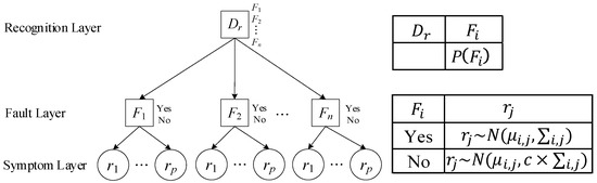
Figure 1.
The structure and parameters of residual-driven BN.
The structure includes three layers, from top to bottom: the recognition layer, the fault layer, and the symptom layer. The recognition layer contains one top node , the fault layer contains fault nodes (), and each fault node is connected to residual nodes () in the symptom layer. The top node has states corresponding to known faults. Each fault node has two states: Yes and No, representing the occurrence and non-occurrence of faults, respectively. Each residual node represents a continuous node consisting of the feature residuals. The residual node enables the utilization of feature residuals.
Its parameters include the prior probabilities of the top node and the conditional probabilities of each sub-node. For the BN shown in Figure 1, the prior probability of each state of the top node can be determined by expert experience or statistical samples. The assignment principle of the conditional probabilities of the fault node given the top node state is shown in Equation (1):
The conditional probability of the residual node is assumed to follow a Gaussian distribution. The two parameters that describe the distribution, mean () and covariance (), given the parent node state, need to be obtained through maximum likelihood estimation from historical data of feature residuals belonging to the fault . The coefficient in Figure 1 is used to determine the conditional probability distribution of the sub-node when the state of the node is No, and its calculation is shown in Equations (2) and (3). The detailed demonstration and validity of Equations (2) and (3) have been presented in the works of Wang et al. [25] and Verron et al. [27].
In the equations, represents the dimension of node , . represents the number of samples, and represents the percentile of the Fisher distribution with degrees of freedom and . is the significance level, which is determined through multiple attempts based on the principle of obtaining optimal diagnostic performance.
2.2. BN Driven by Data
The data-driven approach typically involves constructing a black-box model to establish the mapping relationship between input features and output faults. This approach requires a significant amount of data for training the models. The structure and parameters of the data-driven BN are illustrated in Figure 2.
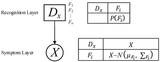
Figure 2.
The structure and parameters of data-driven BN.
The structure includes two layers, from top to bottom: the recognition layer and the symptom layer, each of which includes one top node and one data node X, respectively. The top node has the same states as the top node in Figure 1; the data node X is a continuous node composed of features. The data node X implements the use of feature data.
For the BN parameters, the prior probabilities of the top node are exactly the same as those of the top node in Figure 1. Assuming that the conditional probability of the data node X follows a multidimensional Gaussian distribution, the way to determine the distribution is exactly the same as that of the residual node in Figure 1. Specifically, the two parameters that describe the distribution are the mean vector () and the covariance matrix (), which need to be obtained through maximum likelihood estimation from the feature measurement data belonging to the fault .
2.3. BN Driven by the Fusion of Residuals and Data
The objective of this section is to combine the residual-driven model (Figure 1) with the data-driven model (Figure 2) into a unified BN. Typically, the BN structure is determined by establishing causal relationships between nodes. For complex systems with unclear internal mechanisms, it can be challenging to clarify these causal relationships, requiring the use of optimization algorithms for BN structure learning [28]. However, in the case of chillers, their thermodynamic principles are relatively well-defined, and the influence relationship between typical faults and features is generally understood. Therefore, there is no need to employ structure learning algorithms to determine the BN structure. The structure and parameters of the hybrid BN are depicted in Figure 3. It consists of four layers, namely the decision layer, recognition layer, fault layer, and symptom layer. The configuration of each layer is as follows:
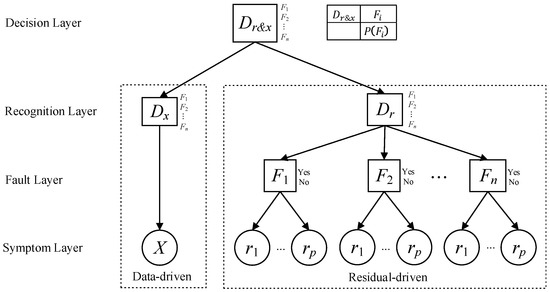
Figure 3.
The structure and parameters of the hybrid BN driven by residual and data.
The function of the symptom layer is to acquire feature residuals and feature data, which serve as evidence for fault diagnosis. With the fusion of the residual-driven and data-driven components, the symptom layer now encompasses both residual nodes and data nodes.
The fault layer plays a critical role in evaluating the evidence obtained from the symptom layer and estimating the probabilities of each fault occurrence. It is specifically included in the residual-driven part of the diagnostic model. This distinction is made because the data-driven part involves numerous features, and almost all faults affect these features. Introducing individual fault nodes, as in the residual-driven part, for each fault in the data-driven part would substantially increase the complexity of model parameter configuration and reduce computational efficiency. Hence, fault nodes are only established separately in the residual-driven part, where the number of features is relatively smaller.
The recognition layer plays a crucial role in inferring the posterior probabilities of each fault by utilizing the posterior probabilities propagated from the fault layer or symptom layer. In the hybrid model combining the residual-driven and data-driven components, the recognition layer consists of two nodes, and , which represent the inference results from the respective parts.
In the diagnostic network presented in Figure 3, the two components involved in the fusion process perform parallel inference computations. Each component independently receives data from the corresponding nodes in its own section of the symptom layer and conducts fault diagnosis in parallel. This parallel inference leads to the generation of separate inference results in the identification layer. To complete the fusion of the identification results from both components, a new top node, , is introduced. The decision layer, as depicted in Figure 3, plays a critical role in combining and consolidating the diagnostic outcomes obtained from the parallel inference calculations performed by the two components. The proposed diagnostic process, which integrates residual-driven and data-driven models within a unified diagnostic framework, is referred to as a hybrid diagnostic method. The effectiveness of this framework has been confirmed in the study conducted by Atoui et al. [29].
The decision layer, represented by node , is a discrete node with the same states as nodes and . To ensure fairness and avoid bias towards any particular state, equal prior probabilities are assigned to each state of node . The principle for assigning conditional probabilities to nodes and in the identification layer follows the same approach. An example of this can be seen in Equation (4), which pertains to node .
The assignment principles for the fault nodes , residual nodes , and data nodes remain consistent with the principles used in the residual-driven and data-driven BN.
2.4. Working Mechanism of Residuals and Data in the Hybrid BN
In this paper, both feature residuals and feature data are utilized to diagnose faults by integrating them into a BN. BN is a probabilistic inference model that employs Bayesian inference to calculate posterior probabilities, specifically , where represents an unobserved state, and represents an observed state with the observed value of . When an event occurs, it serves as evidence (an observed state). When evidence is fed into the BN, the information provided by the evidence is propagated throughout the network to update knowledge and obtain posterior probabilities of the unobserved states. This process is known as inference. BN uses predefined conditional probability distributions and observed evidence for inference.
In BN, the relationships between nodes are represented by the structure and conditional probability distributions. The structure of the BN is determined by the causal relationships between nodes, while the conditional probability distributions are derived from training data. Hence, when integrating feature residuals and feature data into the BN, there is no requirement to explicitly assign weights to these components. In practical applications, BN inherently considers the trade-off between feature residuals and feature data during the computation of posterior probabilities. This means that the diagnostic system automatically takes into account the relative importance and contribution of each type of information. Therefore, it avoids the uncertainty and potential bias that could arise from subjective weight assignments.
It is challenging to theoretically or mathematically show that the simultaneous use of both types of nodes is able to yield better diagnostic performance than using a single type of node, as it involves the complexity of the model and specific data distributions. However, it can be explained through the following reasonable inference.
For a newly observed sample, there are two possible outcomes when it is diagnosed separately by the two types of nodes. The first outcome is that both types of nodes diagnose the sample as the same fault. The second outcome is that the two types of nodes diagnose the sample as having different faults. Integrating the two types of nodes does not affect the first outcome but does impact the second outcome.
For example, let us consider a new observed sample, denoted as , which is diagnosed by the residual node as fault , while the data node diagnoses is as fault . Moreover, the posterior probability of sample being diagnosed as fault by the residual node is only slightly lower than the posterior probability of it being diagnosed as fault . This indicates that the residual node has some ambiguity in diagnosing sample . In this scenario, if the data node unequivocally diagnoses sample as fault , then when both types of nodes are used, sample will be unequivocally diagnosed as fault . If the sample indeed belongs to fault , then the diagnostic result is correct.
This inference process illustrates that when both types of nodes are simultaneously used, it captures more samples that are ambiguously diagnosed by the single-type nodes, thereby improving the diagnostic performance.
3. Framework Based on BN Driven by the Fusion of Residuals and Data
The diagnostic process, driven by the fusion of residuals and data, is illustrated in Figure 4, which consists of two main parts: construction of the hybrid BN model and online fault diagnosis.
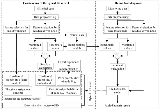
Figure 4.
Framework of the fault diagnosis based on hybrid BN driven by residual and data.
3.1. Construction of the Hybrid BN Model
Construction of the hybrid BN model involves the following steps:
- i
- Data preprocessing and feature selection: The first step is to preprocess the historical data, which encompasses normal operating conditions and different fault types. This process entails removing any obvious transients and anomalies present in the data. Subsequently, appropriate features are selected for both the residual node and the data node .
- ii
- Development of the benchmark model and calculation of feature residuals: By using the normal data as a reference, a benchmark model is constructed for the selected features. Subsequently, the feature residuals are computed by quantifying the deviation between the measured values of each feature and their corresponding benchmark values for each fault scenario.
- ii
- Construction of the hybrid BN driven by residuals and data: Firstly, the structure of the hybrid BN, as depicted in Figure 3, is determined. Next, the prior probability of the top node is established, taking into account expert knowledge or sample statistics. By using the predefined assignment principle, the conditional probabilities of nodes , , and the fault layer nodes are sequentially determined. Finally, the conditional probability distributions of the residual node and the data node X are estimated using maximum likelihood estimation, utilizing the feature residuals and the feature data.
By following these steps, the hybrid BN model is constructed, integrating the residual-driven and data-driven components. This model effectively merges the information from both feature residuals and feature data, allowing for accurate fault diagnosis and analysis.
3.2. Online Fault Diagnosis
In the practical application of the hybrid BN, the real-time monitored data undergo a two-step inference process.
In the first step, the data are input into the symptom layer, where they acquire the feature residuals from the residual-driven part and the feature data from the data-driven part. Through BN inference calculations, the posterior probabilities of the fault layer node in the residual-driven part and the recognition layer node in the data-driven part are obtained.
In the second step, based on the posterior probabilities of the fault layer node , the BN inference calculation is performed again to obtain the posterior probabilities of the recognition layer node in the residual-driven part. These posterior probabilities, along with the posterior probabilities of the recognition layer node from the data-driven part, are propagated to the top layer. Finally, through further inference, the posterior probabilities of the decision layer node are calculated.
According to the principle of maximum posterior probability, the state with the highest posterior probability of the node is outputted as the fault diagnosis result. This ensures that the hybrid BN effectively combines the information from both the residual-driven and data-driven parts, enabling accurate fault diagnoses.
The BN inference algorithm includes two types: the exact inference algorithm and the approximate inference algorithm. Since the hybrid BN developed in this paper is not too complex, the exact inference algorithm, specifically the junction tree algorithm, is used.
4. Application and Performance Evaluation
In this section, the effectiveness and feasibility of the proposed hybrid method are evaluated by applying it to a real-world chiller system used in the ASHRAE RP-1043 project [19], as well as an actual maglev centrifugal chiller. The diagnostic performance of the proposed method is compared with that of existing advanced diagnostic methods.
4.1. Experimental Data
The ASHRAE RP-1043 project [19] used a centrifugal chiller with a cooling capacity of approximately 316 kW. Both the evaporator and condenser were shell-and-tube heat exchangers, with water flowing inside the tubes, and the refrigerant used was R134a, with a thermal expansion valve. The experiments were conducted under 27 operating conditions, and 64 parameters were measured and stored at 10 s intervals, including temperature, pressure, flow, power, etc. Through experiments, a large amount of data was obtained for the normal state of the unit and seven typical faults under four levels of degradation. These faults included reduced condenser water flow (RedCdW), reduced evaporator water flow (RedEvW), refrigerant leak (RefLeak), refrigerant overcharge (RefOver), condenser fouling (CdFoul), noncondensable gas in refrigerant (NcG), and excess oil (ExOil).
4.2. Data Preprocessing and Feature Selection
The data preprocessing method proposed in Ref. [30] was used to perform steady-state filtering on the original experimental data, filtering out any obvious dynamic and abnormal data. Three variables, namely the inlet and outlet temperatures of the chilled water and the inlet temperature of the cooling water, were chosen as the indicators for steady-state filtration.
After steady-state screening, for the normal samples and the samples including faults under four degradation levels, two-thirds of the steady-state data were randomly selected to form the training set, and the remaining one-third of the steady-state data were used for the testing set. For normal and each type of fault under each degradation level, there were approximately 800 and 400 samples in the training and testing sets, respectively. In total, the training set consisted of 23,200 samples, and the testing set consisted of 11,600 samples. This process of dividing the data into training and testing sets was repeated five times, resulting in five sets of training and testing data. Each of these five datasets was used separately to validate the diagnostic performance of the proposed method, providing a more comprehensive demonstration of its effectiveness. The training dataset was used to determine the model parameters, while the testing dataset was used to test and evaluate the diagnostic performance of the model.
Firstly, the features of the residual nodes in the residual-driven part were selected. By referring to previous research findings [18,31,32], a set of fault-sensitive features and their corresponding calculations were determined. These features constitute the residual nodes and are listed in Table 1. For detailed explanations of each feature, please refer to Table 2. Additionally, the association between features and faults can be found in Figure 5.

Table 1.
Features selected by the residual node in residual-driven part.
Table 2.
Features selected by the data node in data-driven part.
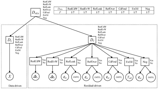
Figure 5.
The structure and parameters of the hybrid method driven by residual and data.
Secondly, the features for the data nodes X in the data-driven part were selected. Considering the results of surveys conducted by Wang et al. [33] regarding the installation status of sensors in on-site chillers, features that are readily available are selected to form the data nodes X. The selected features are presented in Table 2.
4.3. Development of Benchmark Model
To determine the conditional probability distribution of the residual nodes in the symptom layer, a benchmark model first needs to be constructed. Typically, for a fixed water flow rate system, the performance of a chiller can be represented as a relationship between (cooling capacity), , and . Therefore, the features listed in Table 1 are expressed as functions of these three parameters, as shown in Equation (5). This relationship has been proven effective in previous studies [31,32].
where represents the benchmark values of the features listed in Table 1, and .
The task of determining benchmark values for these features can be transformed into a regression-based prediction problem. Previous studies have utilized various regression methods, including multiple linear regression, radial basis function, and support vector regression, for this purpose. In this study, the radial basis function was chosen as the regression method for building the benchmark models based on the comparative analysis conducted by Tran et al. [34]. The benchmark models were constructed with three layers: the input layer, the hidden layer, and the output layer. The input layer consists of three nodes corresponding to , , and . The number () of nodes in the hidden layer was determined by , where is the number of nodes in the input layer. Therefore, in this case, . The output layer comprises five nodes representing the five features listed in Table 1. The weight range between the input layer and the hidden layer was set to [0, 1].
The benchmark models were trained using normal samples from the training set and tested using normal samples from the testing set. The goodness-of-fit of the models was evaluated based on the R-squared () value, where a value closer to 1 indicates better prediction performance. The test results are presented in Table 3, demonstrating the favorable overall prediction performance of the radial basis function-based benchmark models.
Table 3.
Fitting accuracies of the benchmark models based on radial basis function.
4.4. Establishment of the Hybrid BN Driven by Residual and Data
The structure of the hybrid BN is depicted in Figure 5. In order to prevent any bias towards specific states, equal prior probabilities (1/7) were assigned to each state of the top node . The conditional probabilities of the nodes and were determined using Equation (4). The conditional probabilities of each fault node in the fault layer were established based on the assignment principle described in Equation (1). By referring to the relationship between faults and features presented in Table 1, the residual nodes connected to each fault node could be identified. For instance, the features and are sensitive to the RefLeak fault; hence, the residual nodes connected to the RefLeak fault node are the and nodes.
Firstly, the samples corresponding to faults from the training set were input into the trained benchmark models to obtain the benchmark values for each feature. Then, by comparing the benchmark values with the measured values of each feature, the feature residuals were obtained. Maximum likelihood estimation was applied to these feature residuals to derive the conditional probability distributions of the residual nodes. After several attempts, a significance level of 0.025 was chosen, and the value of was calculated using Equations (2) and (3) as 4.
The conditional probability distribution of the data node in the data-driven part was obtained through maximum likelihood estimation using the feature data directly from the training set.
By completing the assignment of prior and conditional probabilities for all nodes in the hybrid BN, the construction of the hybrid BN model was finished.
4.5. Performance Evaluation Indexes
Multiple evaluation metrics were utilized to comprehensively assess the performance of the diagnostic model. These metrics include the confusion matrix, accuracy, precision, recall, and F-measure [35].
By taking the example of a confusion matrix (shown in Table 4) representing a binary classification problem, the calculation of these evaluation metrics is explained. In Table 4, TP represents the number of samples that are true positives (predicted as positive and are actually positive), TN represents the number of samples that are true negatives (predicted as negative and are actually negative), FP represents the number of samples that are false positives (predicted as positive but are actually negative), and FN represents the number of samples that are false negatives (predicted as negative but are actually positive).
Table 4.
Confusion matrix explained by a binary classification problem.
- (1)
- Accuracy
- (2)
- Precision
- (3)
- Recall
- (4)
- F-measure
Precision measures the accuracy of classifying negative samples, indicating the proportion of predicted positive samples that are actually positive. Recall measures the accuracy of classifying positive samples, indicating the proportion of actually positive samples that are correctly predicted as positive. Both precision and recall provide insights into the diagnostic error. F-measure is a harmonic mean that takes into account both precision and recall.
4.6. Fault Diagnosis Results and Discussion
It is important to note that the fault diagnosis results for each scenario were calculated five times using the five datasets formed during the data preprocessing stage. The average of the five computations is presented and discussed as the final fault diagnosis result.
4.6.1. Diagnostic Results Using Only the Residual-Driven Part
In this section, only the feature residuals from the residual-driven part were used for fault diagnosis. The diagnostic performance was evaluated using the data from the testing set, and the test results represented by the confusion matrix are shown in Figure 6, along with the precision, recall, and F-measure. For instance, the precision, recall, and F-measure for RedCdW are determined to be 68.4%, 79.2%, and 73.4%, respectively.
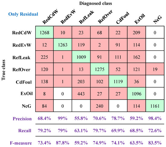
Figure 6.
Confusion matrix representing diagnosis results by using only residual nodes. (The row is the number of samples diagnosed by the method, while the column is the number of actually occurred samples. The correctly diagnosed samples are highlighted in green, and the falsely diagnosed samples are highlighted in red.)
The proposed method achieves a diagnostic accuracy of 73.1% in this scenario. Among the different fault types, the RedEvW and NcG faults exhibit the highest precisions exceeding 90%, while the RefLeak and ExOil faults have the lowest precision, below 60%. The high precision indicates a low false positive rate, meaning that once the fault is diagnosed, there is a high level of confidence that the fault has indeed occurred. The RedCdW, RedEvW, and RefOver faults demonstrate the highest recalls, close to 80%. The high recall indicates a low missed diagnosis rate, meaning that if a fault occurs, it can be accurately diagnosed. Only the RedEvW and NcG faults achieve F-measures above 80%, while the RefLeak fault has the lowest F-measure, at only 59.2%.
These test results validate the effective fusion of the residual-driven model into the hybrid BN model and demonstrate its ability to independently fulfill the diagnostic task only using the feature residual node.
Indeed, the diagnostic performance of using only the residual-driven part for fault diagnosis is strongly affected by the fault-sensitive features listed in Table 1. In this study, the focus was on simplicity and ease of understanding rather than achieving optimal diagnostic performance for the residual-driven part. Therefore, only a small number of features were selected to form the residual nodes.
As shown in Table 1, the selection of the same feature ( and ) for multiple faults (RefLeak, RefOver, CdFoul, and Ncg) has contributed to confusion between these faults. This overlap in feature selection has led to misdiagnosis among these fault types, as evident from the confusion matrix in Figure 6. Consequently, the diagnostic performance for these faults is not satisfactory. However, by incorporating additional fault-sensitive features, the diagnostic performance of the residual-driven part can be effectively enhanced. For example, introducing features such as the difference between the measured condensing temperature and the calculated condensing temperature based on the condensing pressure (which is sensitive to the Ncg fault [18]), including condensing pressure and subcooling (which are highly sensitive to the RefOver, RefLeak, and CdFoul faults [31,36]), or even considering the entropy efficiency of the compressor based on thermodynamic mechanisms and refrigerant flow rate [36,37], can significantly improve the diagnostic accuracy for these specific faults. Furthermore, by combining different types of nodes proposed in this paper, as discussed in Section 4.6.3, the overall fault diagnosis performance can also be further enhanced.
4.6.2. Diagnostic Results Using Only the Data-Driven Part
In this subsection, only feature data from the data-driven part were used for fault diagnosis. The test results, presented in the form of a confusion matrix in Figure 7, demonstrate that the proposed method achieved a high diagnostic accuracy of 94.5% in this case. Among the different fault types, six faults achieved precisions exceeding 90%, with the ExOil fault being the only exception at 86.4%. All seven faults achieved recalls of 80% or higher. Obviously, a low false positive rate and missed diagnosis rate were achieved. The F-measures for six faults are above 90%. The lowest F-measure is observed in the RefLeak fault at 86.1%, which is still considered effective for accurate fault diagnosis.
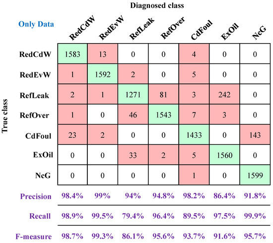
Figure 7.
Confusion matrix representing diagnosis results by using only data nodes (using the same representation as Figure 6).
These test results confirm that the data-driven model is successfully integrated into the hybrid BN model and demonstrate its ability to independently complete the diagnostic task only using the feature data node.
4.6.3. Diagnostic Results Using the Residual-Driven and Data-Driven Parts Together
In this section, feature residuals and feature data from both the residual-driven and data-driven parts were combined for fault diagnosis. The test results, depicted in the form of a confusion matrix in Figure 8, demonstrate that an exceptional diagnostic accuracy of 97.6% was achieved in this case. Among the different fault types, the precisions, recalls, and F-measures for all seven faults were above 90%, indicating an extremely low false positive rate and missed diagnosis rate.
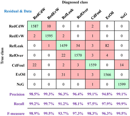
Figure 8.
Confusion matrix representing diagnosis results by using residual and data nodes together (using the same representation as Figure 6).
When comparing the diagnostic results obtained from using only residual nodes or data nodes, it is evident that the diagnostic performance is significantly enhanced when both parts are used together. The diagnostic accuracy improves by up to 24.5%. For individual faults, there is an improvement in precision, recall, and F-measure. The largest improvement in precision is observed for RefLeak, with an increase of 40.5%, while the largest improvement in recall is seen for ExOil, with an increase of 29.4%. As a result, the F-measures for RefLeak and ExOil increased by up to 34.5% and 32.8%, respectively. This improvement can be attributed to the combination of evidence from both types of nodes, allowing for the utilization of more comprehensive information and ultimately enhancing diagnostic performance.
Fully leveraging all available information proves to be an effective approach to improving fault diagnosis performance. The results highlight the effectiveness of fusing residual and data nodes, enabling parallel fault diagnosis with each part independently completing the diagnostic task. When working together, this fusion leads to superior diagnostic performance.
4.7. Performance Comparison with the Latest Advanced Diagnostic Methods
The fault diagnosis performance of the proposed hybrid method was compared with that of the latest advanced methods proposed in similar studies. In order to ensure an impartial and effective comparison, the comparative methods were selected based on the following criteria: (i) they used the same ASHRAE RP-1043 experimental data, and (ii) they employed the latest improved algorithms for model development. As a result, four existing methods were chosen: SLENet-based [15], SP-CNN-based [16], SA-DNN-based [17], and LS-SVM-based [13] methods. These methods are considered to be the most advanced and have been reported to achieve superior diagnostic performance compared to conventional methods.
During the comparison, the proposed method used the same set of features as the comparative methods for fault indication and evaluated the results obtained by jointly utilizing residual and data nodes. The results of the comparison, represented by accuracies and F-measures, are shown in Figure 9 and Figure 10. It is important to note that the performance of the comparative methods is directly sourced from the related literature. The reported performance in these literature sources should represent the best results achieved for the respective comparative methods. For instance, the diagnostic accuracies and F-measures of the SP-CNN-based method are based on the work by Guo et al. [16].
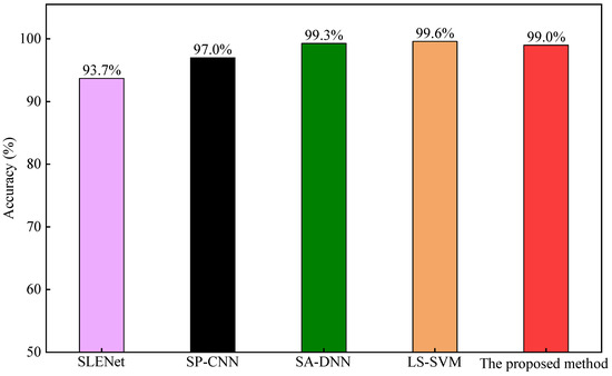
Figure 9.
The comparisons of accuracies among the five diagnostic methods, SLENet from [15], SP-CNN from [16], SA-DNN from [17], LS-SVM from [13].
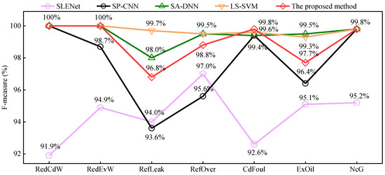
Figure 10.
The comparisons of F-measures among the five diagnostic methods, SLENet from [15], SP-CNN from [16], SA-DNN from [17], LS-SVM from [13].
As depicted in Figure 9 and Figure 10, the diagnostic accuracy of the proposed hybrid method surpasses that of the SLENet-based and SP-CNN-based methods and is on par with the LS-SVM-based and SA-DNN-based methods (with a difference of less than 6%). Regarding F-measures, the proposed hybrid method achieves higher values for all faults compared to the SLENet-based and SP-CNN-based methods. When compared to the LS-SVM-based and SA-DNN-based methods, the proposed hybrid method demonstrates comparable or slightly higher F-measures for all faults, except for RefLeak and ExOil, where the difference is less than 3%.
The training and online diagnosis times of the SVM-based, CNN-based, DNN-based, and proposed methods were calculated and compared. For the model training, all samples from the training set were used, while 100 samples from the testing set were used to simulate an actual fault diagnosis process.
In the case of SVM, the radial basis function was used as the kernel function, and five-fold cross-validation and grid search algorithm were employed to optimize the penalty coefficient and kernel width. The grid searches were conducted within the region of . The CNN architecture consisted of an input layer, two convolutional layers, two activation layers, two pooling layers, one fully connected layer, and an output layer. The rectified linear unit was used as the activation function. The DNN architecture included an input layer, five hidden layers, and an output layer, utilizing the hyperbolic tangent as the activation function. The proposed method incorporated feature residuals and feature data simultaneously for fault diagnosis.
The results are presented in Table 5, indicating that the proposed method requires shorter times for both model training and online diagnosis compared to the SVM-based, CNN-based, and DNN-based models. Particularly for model training, the proposed method demonstrates a significant reduction in time cost ranging from 56.2% to 76.9% compared to the other methods.
Table 5.
The time cost of the model training and online diagnosis for the SVM-based, CNN-based, DNN-based, and proposed methods.
In summary, the proposed hybrid method has two distinct advantages compared to the comparison methods:
- i.
- Method classification: The comparative methods are all data-driven approaches that rely solely on feature data for fault diagnosis. This is similar to the process of the proposed hybrid method when using only data nodes for fault diagnosis. However, the key advantage of the proposed hybrid method is its fusion of additional information, specifically feature residuals, during the fault diagnosis inference process. This fusion of multiple information sources is likely the main reason for the improved fault diagnosis performance.
- ii.
- Model complexity and training cost: The comparative methods incorporate optimization algorithms to optimize model parameters or select the best features to enhance their performance. This, to some extent, increases the complexity of the models and the training cost. The shorter training and application times of the proposed hybrid method provide an additional advantage. The performance comparison results with existing advanced diagnostic methods further validate the effectiveness and superiority of the proposed hybrid method.
4.8. Application of the Proposed Method in Another Chiller
To further validate the effectiveness of the proposed hybrid method, it was applied to another magnetic centrifugal chiller with a cooling capacity of approximately 440 kW. This chiller also featured shell-and-tube heat exchangers for both the evaporator and condenser, with water flowing inside the tubes. The refrigerant used was R134a. The experimental setup involved various operating conditions, including different set points for the chilled water outlet temperature (5 °C, 7 °C, 8 °C, and 10 °C), cooling water inlet temperatures (25 °C, 27 °C, 30 °C, and 33 °C), and load ratios (40%, 50%, 60%, 70%, 80%, and 90%). Data were collected from a total of 51 operating conditions during the experiment, with a data acquisition interval of 10 s. A comprehensive dataset comprising measurements from 25 parameters was obtained. The five types of faults conducted in this experiment were RedCdW, RedEvW, RefLeak, RefOver, and CdFoul.
The experimental data from the magnetic centrifugal chiller underwent the same data preprocessing process as the ASHRAE RP-1043 data. However, since the magnetic centrifugal chiller was an oil-free system, parameters related to lubricating oil were excluded during the feature selection process. The test results demonstrate that the proposed hybrid method achieves an accuracy of 98.3% when both the residual and data nodes were used for fault diagnosis. The F-measures for fault diagnosis were calculated and presented in Table 6. The results reveal that all F-measures for the five faults exceed 95%, providing further evidence of the excellent diagnostic performance of the proposed hybrid method.
Table 6.
The F-measures when both the residual and data nodes were used in the maglev chiller.
4.9. Analysis of the Potential for Field Application of the Proposed Hybrid Method
By applying the proposed method to two actual chillers, it was demonstrated that the method achieves a high diagnostic accuracy of 97.6%. Moreover, when both feature residuals and feature data are used jointly, the method achieves precisions, recalls, and F-measures above 90% for all seven faults. These results indicate the effectiveness and reliability of the proposed method in fault diagnosis.
Furthermore, when compared to existing state-of-the-art methods, the proposed method shows comparable, and in some cases, even superior, diagnostic performance with higher accuracy and F-measure. This highlights the potential of the proposed method to outperform existing methods in practical applications.
The successful application of the proposed method on two actual chillers, the use of readily available features, and the shorter training and application times further demonstrate the feasibility and practicality of the method in real-world scenarios.
In addition to its strong diagnostic performance, the proposed hybrid method also exhibits great potential for practical application in the field. By utilizing feature residuals and feature data in parallel, the method is designed to be robust and tolerant towards any missing parts of the information. For instance, in situations where obtaining an accurate benchmark model is challenging or impractical, the evidence provided by the feature residuals may be unavailable. In such cases, the proposed hybrid method can still perform fault diagnosis by relying solely on the evidence from the feature data. Similarly, if feature data are unavailable or incomplete, the method can utilize only the feature residuals for diagnostic purposes. This flexibility in data utilization enhances the adaptability and robustness of the proposed hybrid method in practical scenarios.
Furthermore, when both feature residuals and feature data are available, the proposed hybrid method can leverage both sources of information simultaneously, resulting in optimal diagnostic performance and making it a promising solution for on-site fault diagnosis in chillers.
5. Conclusions
To effectively leverage the information from both feature residuals and feature data within a unified diagnostic system, a hybrid method based on BN is proposed. The effectiveness and superiority of the proposed hybrid method were validated through its application to two actual chillers. The main conclusions are as follows:
- (1)
- The hybrid method not only enables independent diagnosis using either type of node but also allows for joint diagnosis using both feature residuals and feature data. This capability leads to improved diagnostic performance and enhances the field applicability of the method compared to approaches that solely rely on one type of node.
- (2)
- The hybrid method demonstrates favorable diagnostic performance when utilizing either feature residuals or feature data alone. However, significant improvements in diagnostic performance are observed when both types of nodes are used together. For instance, the accuracy increases to 97.6%, exhibiting a maximum improvement of 24.5%. The precisions, recalls, and F-measures for all seven faults are above 90%, indicating an extremely low false positive rate and missed diagnosis rate. Moreover, the F-measure shows notable enhancements of 34.5% and 32.8% for the challenging-to-diagnose faults of RefLeak and ExOil, respectively. By integrating evidence from both types of nodes, the hybrid method effectively utilizes a wider range of information, surpassing the diagnostic capabilities of using a single type of node alone and leading to enhanced diagnostic performance.
- (3)
- n comparison to the latest advanced methods, the hybrid method has demonstrated comparable, and in some cases, even superior diagnostic performance with higher accuracy and F-measures. Additionally, the proposed method requires shorter training and application times for the model, further highlighting its effectiveness and superiority.
- (4)
- The application of the hybrid method on another actual chiller further validates its effectiveness, achieving a diagnostic accuracy of 98.3% and F-measures above 95% for all considered faults.
Author Contributions
Conceptualization, Z.W.; Methodology, Z.W.; Software, B.L., J.G. and X.L.; Validation, Z.W. and B.L.; Formal analysis, Z.W. and L.W.; Investigation, J.G. and Y.T.; Resources, Y.T.; Data curation, B.L.; Writing—original draft, B.L.; Writing—review & editing, Z.W., X.L. and S.Z.; Visualization, J.G.; Supervision, L.W. All authors have read and agreed to the published version of the manuscript.
Funding
The authors gratefully acknowledge the support of the National Natural Science Foundation of China (No.51806060, No.51876055), the Program for Science & Technology Innovation Talents in Universities of Henan Province (No.22HASTIT025), and the Program for Innovative Research Team (in Science and Technology) in University of Henan Province (No. 22IRTSTHN006).
Data Availability Statement
No new data were created or analyzed in this study. Data sharing is not applicable to this article.
Conflicts of Interest
The authors declare no conflict of interest.
Abbreviations
| CNN | Convolutional neural network |
| BN | Bayesian network |
| DNN | Deep neural network |
| SVM | Support vector machine |
| LS-SVM | Least squares support vector machine |
| SA | Simulated annealing |
| SLENet | Sparsely local embedding CNN |
| SP-CNN | Data self-production algorithm with CNN |
| RedCdW | Reduced condenser water flow |
| RedEvW | Reduced evaporator water flow |
| RefLeak | Refrigerant leakage |
| RefOver | Refrigerant overcharge |
| CdFoul | Condenser fouling |
| NcG | Non-condensable gas in refrigerant |
| ExOil | Excess oil |
References
- Nalley, S. Annual Energy Outlook 2021; Energy Information Administration: Washington, DC, USA, 2021.
- Katipamula, S.; Brambley, M.R. Methods for fault detection, diagnostics, and prognostics for building systems—A review, Part I. HVAC&R Res. 2005, 11, 3–25. [Google Scholar]
- Browne, M.W.; Bansal, P.K. Different modelling strategies for in situ liquid chillers. Proc. Inst. Mech. Eng. Part A J. Power Energy 2001, 215, 357–374. [Google Scholar] [CrossRef]
- Zhao, Y.; Wang, S.; Xiao, F.; Ma, Z. A simplified physical model-based fault detection and diagnosis strategy and its customized tool for centrifugal chillers. HVAC&R Res. 2013, 19, 283–294. [Google Scholar]
- Kim, W.; Braun, J.E. Extension of a virtual refrigerant charge sensor. Int. J. Refrig. 2015, 55, 224–235. [Google Scholar] [CrossRef]
- Kim, W.; Braun, J.E. Development and evaluation of virtual refrigerant mass flow sensors for fault detection and diagnostics. Int. J. Refrig. 2016, 63, 184–198. [Google Scholar] [CrossRef]
- Chen, J.; Zhang, L.; Li, Y.; Shi, Y.; Gao, X.; Hu, Y. A review of computing-based automated fault detection and diagnosis of heating, ventilation and air conditioning systems. Renew. Sustain. Energy Rev. 2022, 161, 8112395. [Google Scholar] [CrossRef]
- Yan, K.; Ma, L.; Dai, Y.; Shen, W.; Ji, Z.; Xie, D. Cost-sensitive and sequential feature selection for chiller fault detection and diagnosis. Int. J. Refrig. 2018, 86, 401–409. [Google Scholar] [CrossRef]
- Li, G.; Yao, Q.; Fan, C.; Zhou, C.; Wu, G.; Zhou, Z.; Fang, X. An explainable one-dimensional convolutional neural networks based fault diagnosis method for building heating, ventilation and air conditioning systems. Build. Environ. 2021, 203, 108057. [Google Scholar] [CrossRef]
- Chen, K.; Wang, Z.; Gu, X.; Wang, Z. Multicondition operation fault detection for chillers based on global density-weighted support vector data description. Appl. Soft Comput. 2021, 112, 107795. [Google Scholar] [CrossRef]
- Liu, J.; Shi, D.; Li, G.; Xie, Y.; Li, K.; Liu, B.; Ru, Z. Data-driven and association rule mining-based fault diagnosis and action mechanism analysis for building chillers. Energy Build. 2020, 216, 109957. [Google Scholar] [CrossRef]
- Guo, Y.; Liu, J.; Liu, C.; Zhu, J.; Lu, J.; Li, Y. Operation Pattern Recognition of the Refrigeration, Heating and Hot Water Combined Air-Conditioning System in Building Based on Clustering Method. Processes 2023, 11, 812. [Google Scholar] [CrossRef]
- Han, H.; Cui, X.; Fan, Y.; Qing, H. Least squares support vector machine (LS-SVM)-based chiller fault diagnosis using fault indicative features. Appl. Therm. Eng. 2019, 154, 540–547. [Google Scholar] [CrossRef]
- Han, H.; Cui, X.; Fan, Y.; Qing, H. Ensemble learning with member optimization for fault diagnosis of a building energy system. Energy Build. 2020, 226, 110351. [Google Scholar] [CrossRef]
- Liu, X.; Li, Y.; Sun, S.; Liu, X.; Shen, J. Fault diagnosis of chillers using sparsely local embedding deep convolutional neural network. CIESC J. 2018, 69, 5155–5163. [Google Scholar]
- Gao, J.; Han, H.; Ren, Z.; Fan, Y. Fault diagnosis for building chillers based on data self-production and deep convolutional neural network. J. Build. Eng. 2021, 34, 102043. [Google Scholar] [CrossRef]
- Han, H.; Xu, L.; Cui, X.; Fan, Y. Novel chiller fault diagnosis using deep neural network (DNN) with simulated annealing (SA). Int. J. Refrig. 2021, 121, 269–278. [Google Scholar] [CrossRef]
- Wang, Z.; Wang, L.; Tan, Y.; Yuan, J.; Li, X. Fault diagnosis using fused reference model and Bayesian network for building energy systems. J. Build. Eng. 2021, 34, 101957. [Google Scholar] [CrossRef]
- Comstock, M.C.; Braun, J.E.; Bernhard, R. Development of Analysis Tools for the Evaluation of Fault Detection and Diagnostics for Chillers; ASHRAE Research Project 1043-RP, HL 99-20, Report #4036-3; Purdue University: West Lafayette, IN, USA, 1999. [Google Scholar]
- Li, T.; Zhao, Y.; Zhang, C.; Luo, J.; Zhang, X. A knowledge-guided and data-driven method for building HVAC systems fault diagnosis. Build. Environ. 2021, 198, 107850. [Google Scholar] [CrossRef]
- Wang, P.; Li, C.; Liang, R.; Yoon, S.; Mu, S.; Liu, Y. Fault detection and calibration for building energy system using Bayesian inference and sparse autoencoder: A case study in photovoltaic thermal heat pump system. Energy Build. 2023, 290, 113051. [Google Scholar] [CrossRef]
- Li, G.; Xiong, J.; Tang, R.; Sun, S.; Wang, C. In-situ sensor calibration for building HVAC systems with limited information using general regression improved Bayesian inference. Build. Environ. 2023, 234, 110161. [Google Scholar] [CrossRef]
- Chen, Y.; Wen, J.; Pradhan, O.; Lo, L.J.; Wu, T. Using discrete Bayesian networks for diagnosing and isolating cross-level faults in HVAC systems. Appl. Energy 2022, 327, 120050. [Google Scholar] [CrossRef]
- Hu, M.; Chen, H.; Shen, L.; Li, G.; Guo, Y.; Li, H.; Li, J.; Hu, W. A machine learning Bayesian network for refrigerant charge faults of variable refrigerant flow air conditioning system. Energy Build. 2018, 158, 668–676. [Google Scholar] [CrossRef]
- Wang, Z.; Wang, Z.; He, S.; Gu, X.; Yan, Z.F. Fault detection and diagnosis of chillers using Bayesian network merged distance rejection and multi-source non-sensor information. Appl. Energy 2017, 188, 200–214. [Google Scholar] [CrossRef]
- Wang, Z.; Wang, L.; Tan, Y.; Yuan, J. Fault detection based on Bayesian network and missing data imputation for building energy systems. Appl. Therm. Eng. 2021, 182, 116051. [Google Scholar] [CrossRef]
- Verron, S.; Tiplica, T.; Kobi, A. Fault diagnosis of industrial systems by conditional Gaussian network including a distance rejection criterion. Eng. Appl. Artif. Intell. 2010, 23, 1229–1235. [Google Scholar] [CrossRef]
- Tan, X.; Gao, X.; Wang, Z.; Han, H.; Liu, X.; Chen, D. Learning the structure of Bayesian networks with ancestral and/or heuristic partition. Inf. Sci. 2022, 574, 719–775. [Google Scholar] [CrossRef]
- Atoui, M.A.; Verron, S.; Kobi, A. A Bayesian network dealing with measurements and residuals for system monitoring. Trans. Inst. Meas. Control 2016, 38, 373–384. [Google Scholar] [CrossRef]
- Kim, M.; Yoon, S.H.; Domanski, P.A.; Payne, W.V. Design of a steady-state detector for fault detection and diagnosis of a residential air conditioner. Int. J. Refrig. 2008, 31, 790–799. [Google Scholar] [CrossRef]
- Xiao, F.; Zheng, C.; Wang, S.W. A fault detection and diagnosis strategy with enhanced sensitivity for centrifugal chillers. Appl. Therm. Eng. 2011, 31, 3963–3970. [Google Scholar] [CrossRef]
- Zhao, Y.; Wang, S.; Xiao, F. A statistical fault detection and diagnosis method for centrifugal chillers based on exponentially-weighted moving average control charts and support vector regression. Appl. Therm. Eng. 2013, 51, 560–572. [Google Scholar] [CrossRef]
- Wang, Z.; Wang, Z.; Gu, X.; He, S.; Yan, Z. Feature selection based on Bayesian network for chiller fault diagnosis from the perspective of field applications. Appl. Therm. Eng. 2018, 129, 674–683. [Google Scholar] [CrossRef]
- Tran, D.A.T.; Chen, Y.; Jiang, C. Comparative investigations on reference models for fault detection and diagnosis in centrifugal chiller systems. Energy Build. 2016, 133, 246–256. [Google Scholar] [CrossRef]
- Zhu, H.; Yang, W.; Li, S.; Pang, A. An Effective Fault Detection Method for HVAC Systems Using the LSTM-SVDD Algorithm. Buildings 2022, 12, 246. [Google Scholar] [CrossRef]
- Zhou, Q.; Wang, S.; Xiao, F. A Novel Strategy for the Fault Detection and Diagnosis of Centrifugal Chiller Systems. HVAC&R Res. 2009, 15, 57–75. [Google Scholar]
- Cui, J.; Wang, S. A model-based online fault detection and diagnosis strategy for centrifugal chiller systems. Int. J. Therm. Sci. 2005, 44, 986–999. [Google Scholar] [CrossRef]
Disclaimer/Publisher’s Note: The statements, opinions and data contained in all publications are solely those of the individual author(s) and contributor(s) and not of MDPI and/or the editor(s). MDPI and/or the editor(s) disclaim responsibility for any injury to people or property resulting from any ideas, methods, instructions or products referred to in the content. |
© 2023 by the authors. Licensee MDPI, Basel, Switzerland. This article is an open access article distributed under the terms and conditions of the Creative Commons Attribution (CC BY) license (https://creativecommons.org/licenses/by/4.0/).