Abstract
In this work, deep reinforcement learning methodology takes advantage of transfer learning methodology to achieve a reasonable trade-off between environmental impact and operating costs in the activated sludge process of Wastewater treatment plants (WWTPs). WWTPs include complex nonlinear biological processes, high uncertainty, and climatic disturbances, among others. The dynamics of complex real processes are difficult to accurately approximate by mathematical models due to the complexity of the process itself. Consequently, model-based control can fail in practical application due to the mismatch between the mathematical model and the real process. Control based on the model-free reinforcement deep learning (RL) methodology emerges as an advantageous method to arrive at suboptimal solutions without the need for mathematical models of the real process. However, convergence of the RL method to a reasonable control for complex processes is data-intensive and time-consuming. For this reason, the RL method can use the transfer learning approach to cope with this inefficient and slow data-driven learning. In fact, the transfer learning method takes advantage of what has been learned so far so that the learning process to solve a new objective does not require so much data and time. The results demonstrate that cumulatively achieving conflicting objectives can efficiently be used to approach the control of complex real processes without relying on mathematical models.
1. Introduction
Model-based controller design and analysis require mathematical models of the real process to be controlled for successful development and implementation. Advanced control, such as model-based predictive control (MPC), has provided stability, robustness, and good performance to control systems. Basically, the mathematical models of complex non-linear processes are approximation models of the real process. However, these approximation models involve a model mismatch with the real process due to the complex dynamics and uncertainties included in the process, which cannot be obtained quantitatively or qualitatively by physical or identification modeling. Accordingly, model-based controllers are not guaranteed successful performance in real implementations.
Wastewater treatment plants (WWTPs) involve complex nonlinear biological processes impacted by weather disturbances, influent uncertainty, difficult-to-predict external factors, and faulty sensors, among others. In recent years, interest in the problems of the operation and control of wastewater treatment plants has increased due to the increasingly demanding regulations on water quality. The activated sludge process (ASP) is the most widely used biological process for mathematical models of wastewater treatment plants. In ASP, sludge is bacteria in suspension, called biomass, that remove contaminants. In particular, the Activated Sludge Model n°1 (ASM1) introduces nitrogen and organic matter removal based on oxygen and nitrate consumption. In these cases, the control of oxygen [1] is the most studied by researchers due to its strong and rapid influence on the sludge within the ASP [2]. Different model-based control strategies have been developed using ASM models [3,4,5]. Nonetheless, the ASM models do not represent the real process models exactly. Consequently, although MPC is a powerful tool for dynamically controlling processes, control systems designed under these simulation models may fail in the real process due to the high uncertainty caused by the biological process, making its deployment in real applications difficult.
In real WWTPs control, a human field operator replies to uncertainty and all the above factors, taking advantage of their experience. Accordingly, we considered it necessary to develop computational intelligence systems proficient at recreating a control role similar to the expert human operator to bring some autonomy to the operational performance of wastewater treatment processes.
Reinforcement learning (RL) is a machine learning methodology that includes data-driven techniques and algorithms to solve optimal control problems using sequential decisions [6,7]. Instead of hard-programming the solution for the controllers, an RL agent learns a desired decision strategy as a human brain through a trial-and-error process. More precisely, this RL agent learns by interacting with the environment: the environment sends a state, the agent responds with an action based on a decision strategy, and the environment responds with a new state and a reward. The new state is the consequence of the action. At the same time, the reward is a scalar value indicative of how good the decision strategy of the agent is. The interaction aims to reach a decision strategy that maximizes the cumulative discounted reward.
In fact, reinforcement learning is the meeting point between control theory and machine learning. On the one hand, RL control theory [7], basically dynamic programming and Bellman optimality, allow for dividing a complex problem into sequentially sub-problems. On the other hand, machine learning and deep learning provide deep neural networks known to contain universal approximation properties. Therefore, from a broader perspective, deep reinforcement learning [8] can employ deep neural networks to address complex a priori unknown environments within high dimension of states and action continuous. Deep reinforcement learning falls into two main categories, value-based and policy-based. In the first one, it optimizes the Q function in search of the action with the maximum Q value given a state applying a policy. The second directly optimizes the policy that maximizes the cumulative discounted reward. For example, the value-based deep Q-network algorithm approximates the Q function using a deep neuronal network. The policy-based policy gradient algorithm approximates the policy using a deep neuronal network. The policy is the decision strategy of the agent. Accordingly, the deep neural network is iteratively optimized in policy-based algorithms. This self-adaptive nature of model-free RL algorithms makes agents potentially competent at discovering near-optimal solutions without the mathematical models of the process.
However, most RL algorithms face sampling efficiency problems [9], making learning an optimal policy in complex dynamics difficult. Transfer reinforcement learning method reduces the samples needed to achieve a policy by reusing previous knowledge. Basically, transfer reinforcement learning method specifies which information is transferred and how it is transferred in a reinforcement learning method context: [10] reward shaping [11], learning from demonstration [12,13], mapping between tasks [14,15], representational transfer [16,17], and policy transfer [18,19], among others. Transferring a policy can be re-training a policy to achieve a similar objective to the one already achieved. Therefore, this reusing policy approach could be useful in addressing a complex process composed of conflicting sub-objectives.
In recent years, deep reinforcement learning has been applied to diverse engineering fields, particularly in continuous control processes [20,21]. A review of applications of RL in continuous process control processes can be found in [22], and [23] summarizes recent developments in RL and discusses its implications for the process control field. The relationships between model predictive control and reinforcement learning are studied in [24], highlighting their strengths and weaknesses.
Machine learning in wastewater treatment plants [25,26] stands out for predicting the risk of violating pollution legal effluent limits. Thus, supervised networks usually participate as predictors in control strategies focused on avoiding these violations [27,28]. In the case of the RL method, unlike the supervised machine learning method one, there is no explicit knowledge of the desired inputs and outputs. Fundamentally, the desired inputs and outputs are achieved using a reward that indicates the objectives as a guide for the optimization. For example, ref. [29] considers LCA indices using multiagent deep reinforcement learning (MADRL) in order to optimize dissolved oxygen simultaneously and chemical dosage in a WWTP, while [30] gives a previous instruction to the reinforcement learning agent before it acts on the plant for the trade-off between effluent quality and operating costs.
The present proof-of-concept attempts to address multiple gaps and, in doing so, make important contributions:
- This work extends the limited research of model-free reinforcement learning in WWTPs control by implementing a simple policy gradient algorithm to achieve multiple objectives.
- For the first time, it demonstrates transfer reinforcement learning in its basic policy reuse format as an option to address multiple competing objectives in WWTP efficiently.
In this work, controller RL agents are trained by a model-free policy gradient algorithm to achieve a reasonable trade-off between the environmental impact and operating costs in wastewater treatment plants. To this end, we reuse a policy to achieve the global control objective by accumulating the fulfillment of competing sub-objectives: first, reducing the environmental impact, and then operating costs, according to legal limits and performance indexes. More precisely, the control is on the aerobic process to reduce ammonia and nitrate pollution and the aeration energy cost. To demonstrate efficient learning, RL agents that used previous experience are compared with those that did not reuse previous experience. Furthermore, although the proposed agents will be trained and evaluated in Benchmark Simulation Model n°1 (), they will also be evaluated in Benchmark Simulation Model n°2 () [31].
The rest of the paper is organized as follows: Section 2 presents the in which the controller RL agents are trained and evaluated, and the . Section 3 details the problem statement to minimize environmental impact and operation costs. Section 4 defines the deep reinforcement learning algorithm employed and the transfer learning approach. Section 5 presents simulation results. Finally, Section 6 assembles concluding remarks.
2. Plant Description
In this section, protocol and benchmarking software tools used to evaluate the performance and control strategies in waste water treatment plants (WWTPs) are presented.
2.1. Benchmark Simulation Model n°1
The Benchmark Simulation Model n°1 [32] includes the mathematical ASM1 model of the activated sludge process (ASP) [33]. The ASP is a widely used biological treatment process that removes pollutants through sludge composed of bacteria in suspension. The pollutants can be nitrogen and/or phosphorus, in addition to organic carbon substances [34]. Nitrogen is removed in serial stages, de-nitrification, and nitrification, managed by anoxic and aerobic conditions. Figure 1 and Figure 2 show the ASM1 process variables in the BSM1 (except oxygen and the alkalinity ) by the sequential relationship between the variables within the anoxic and aerobic processes, respectively. In particular, nitrogen can be found as ammonium , nitrate , and nitrite . Basically, the process is as follows: first, in de-nitrification, nitrate is reduced to nitrogen gas by heterotrophic bacteria (Figure 1). Then, in nitrification, the ammonia is oxidized to nitrate by autotrophic bacteria (Figure 2). As stated, the role of bacteria is fundamental, but, to carry out its function, it needs oxygen, especially in the nitrification process. Furthermore, it is important to note that the reduction of ammonium involves nitrate increases.
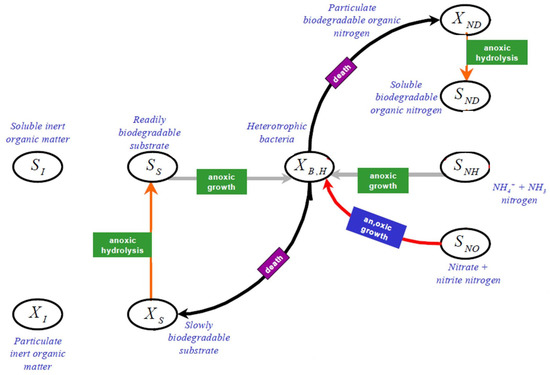
Figure 1.
ASP process variables in the anoxic condition.
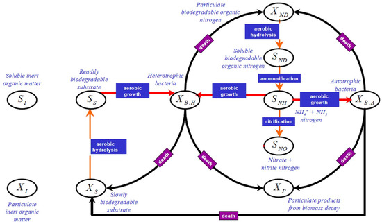
Figure 2.
ASP process variables in the aerobic condition.
The BSM1 includes three influent disturbance profiles: dry, rain, and storm weather. The average influent dry weather flow rate is 18,446 . In particular, each profile contains data from two weeks of simulation with samples every 15 min. The plant layout is as follows: two anoxic reactors (denitrification) with 1000 volume each, three aerobic reactors (nitrification) with 1333 volume each, and a secondary decanter (6000 ). In addition, it includes internal recirculation to ensure nitrates in the anoxic reactors from the aerobic reactors [35] and external recirculation to ensure sludge from the secondary decanter to the anoxic reactors. As for plant control, the default control in Figure 3 is based on the control. More precisely, aeration factor is manipulated in reactor 5, and the internal recirculation is manipulated to arrive at reactor 2. Thus, the oxygen set point is 2 g·m, and the nitrate set point is 1 g·m.
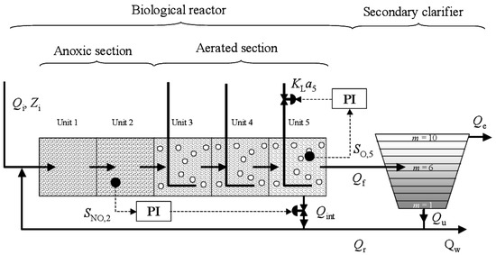
Figure 3.
Benchmark Simulation Model n°1, plant layout and default control.
Oxygen control is fundamental in the control strategies [1], not only because it is needed to ensure the presence of bacteria to remove pollutants but also because of the operating cost linked to its presence. The aerobic process is oxygen-dependent and involves the removal of nitrogen in the structure of ammonia () in reactors 3, 4, and 5 (Figure 3). The oxygen () is food for the bacteria in order to remove ammonia to nitrates, which, by controlled recirculation, is converted to nitrogen gas in the anoxic reactors. Because of the significant and quick effect of oxygen on bacterial growth, concentration is the most studied control in WWTP [36,37].
The mass balance for reactors is defined by the next general equation:
where is the constant volume of the reactor , and the concentration Z with flow Q, is the conversion rate for the component Z. The particularized case of (1) defines the dynamic of according to the next equation:
where is the transfer coefficient, which is the manipulated variable to bring the concentration to desired levels, = 8 [g·m] is the saturation concentration for , and the conversion rate for the So is . As observed in (Equation (2)), the concentration is defined by a complex non-linear dynamic model.
In addition, there is a strong shock of the disturbances in the process, mainly coming from each weather condition. Furthermore, the deal with thirteen state variables; each variable is associated with a conversion ratio resulting from the combination of eight basic processes that define the biological behavior of the system [32]. On the other hand, as an example of the disturbances coming in to the process, Figure 4 and Figure 5 display the flow rate influent and ammonium influent time evolution from day 7 to 14 and sampled every 15 min.
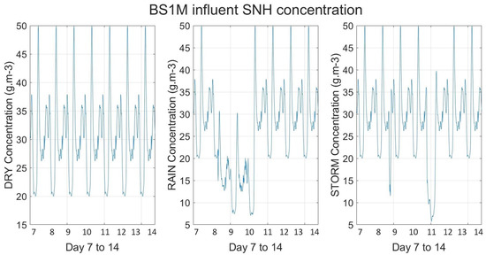
Figure 4.
Influent flow rate disturbances into dry, rain, and storm weather conditions, respectively.
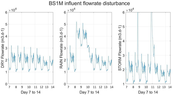
Figure 5.
Influent ammonia disturbances into dry, rain, and storm weather conditions, respectively.
2.2. Benchmark Simulation Model n°2
The Benchmark Simulation Model n°2 (Figure 6) is an extension of the BSM1. Consequently, it represents the following treatments: primary treatment through a settler, secondary treatment (BSM1), and sludge treatment. Also, unlike the BSM1, the plant is designed for an average influent flow in dry weather of 20,648.36 m/day and also considers the temperature seasonal effects within the processes. The volume of each anoxic reactor is 1500 m, and, for each aerobic reactor, it is 3000 m. Furthermore, the secondary settler has a volume of 6000 m. In this case, there is a single influent comprising data corresponding to 609 simulation days and considering temperature, dry, rain, and storm data.
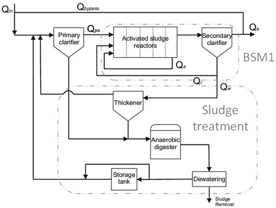
Figure 6.
Benchmark Simulation Model n°2 simplified plant layout.
2.3. Performance Indices
In order to evaluate the control strategies on plant performance, the provides the effluent quality () index and the operating cost index (), also including limits for the concentration of pollutants; Table 1.

Table 1.
Effluent quality limits.
is the weighted average of pollutant concentrations in the effluent:
In turn, is defined as:
where is the aeration energy cost index,
is pumping energy, is sludge production, is external source carbon consumption, and is mixing energy, all of them detailed in [32].
Concerning the limits of the effluent, the ammonia average effluent concentration () is the sum of the discrete levels of divided by the total number of samples, and total nitrogen () is calculated as the sum of and , where is the nitrogen concentration.
3. Problem Statement
Respecting the legal limits of pollution in the effluent is the main objective of wastewater treatment control. On the other hand, efficiently controlling the operation costs to respect these limits is a complementary objective.
The previous section indicates that the BSM1 provides fixed influent disturbances linked to each weather condition, but this is not the case in real WWTP, where other uncertainties are also presented. Consequently, the control carried out by an expert human operator relies on a decision strategy obtained from the accumulated experience according to the operating states of the plant. Therefore, we employed an intelligent agent trained under model-free deep reinforcement learning, taking advantage of previous experience. The objective is the trade-off between effluent quality and operating costs: respecting the legal limits for ammonium and total nitrogen in the effluent, and minimizing aeration energy cost, effluent quality, and operating cost indices defined in the [32].
The control strategy is based on the default control strategy (Section 2); in particular, adding an upper layer to determine the oxygen set points of reactors 3, 4, and 5 (, , and ) that the RL agent will provide. In this sense, controllers PI take the oxygen reference and manipulate their reactor’s oxygen transfer coefficients, , , and . On the anoxic loop side, the nitrate reference sets the constant to 1 g·m.
The oxygen presence leads to a couple of non-beneficial increases: the aeration energy cost index () required to inject oxygen and the nitrates () generated due to ammonia () reduction. Therefore, the controlled variables are in reactor 5 and depend on and normalized by variable scaling, and related to and , respectively, and the oxygen set point (), related to the aeration energy costs ().
For this purpose, it is necessary to consider a trade-off between , a particular case of the trade-off between environmental impact and operating costs in WWTPs. To address effluent quality, minimization of the squared errors of the and concerning the legal limits of ammonia and total nitrogen in the effluent, respectively, is considered. These limits are considered references due to their relationship with each controlled environmental impact variable. Instead, the energy cost of aeration linked to operating costs must also be minimized. Each objective is normalized by variable scaling. Therefore, the objective function takes the following configuration:
Both sub-objectives (Equation (6)) involve conflicts of interest, i.e., the more effluent quality (minimization of and ) we want, the more operating costs (more cost) we will have. Consequently, we will approach the problem in two sequential stages. First, an inexperienced RL agent solves the minimization of and concerning its references. Second, taking advantage of the knowledge obtained to achieve the first, we will approach the minimization of and concerning its references and the minimization of . Nevertheless, also in this work, another RL agent will have as an objective the discrete versions of the effluent quality index Equation (3) and the operating cost index Equation (4) (only PE, AE, and SP are considered).
4. Methodology
The basic elements of training by reinforcement learning methodology are the environment, agent, state, action, and reward. This machine learning methodology is based on optimal control, which includes dynamic programming and Bellman’s optimality principle [7]. Thus, from the control theory outlook, the elements of RL methodology could have their peers: the environment is the controlled system, the RL agent is the controller agent, the states are the controlled variables, the actions are the manipulated variables, and the reward is the cost function.
Considering a standard approach, the environment is modeled as a Markov decision process, a tuple , where is the set of states s, is the set of actions a, is the stochastic transition function, , and the reward function, , and is the initial state. A training episode is a sequence of discrete time steps , where T is the finite horizon. At t, the agent, according to observed state , sends an and receives from the environment a state and a reward , where : the state is the consequence of the action on the environment, and the reward is the qualification of the policy behavior. Hence, the agent sends an action based on a stochastic policy as the definer of its behavior, which maps states to actions . The objective is to achieve a desired policy that maximizes the cumulative discount reward.
The RL methodology has several algorithms to achieve the desired policy, especially for unknown complex dynamics environments with continuous and high-dimensional state S and action A spaces. In deep reinforcement learning, a deep neural network (DNN) can be used as an approximation function of the policy.
4.1. Policy Gradient Algorithm
In this work, we use the policy gradient (PG) algorithm [38]. Because it uses deep neural networks as a function approximation of a stochastic policy, it can learn policies in prior-unknown complex environments with high-dimensional continuous action spaces. In addition, due to its on-policy nature, it directly updates the parameters of the deep neural network. The PG uses the ascendant gradient optimization method [39] to update the parameters of a stochastic policy, a probability distribution of taking action a given a state s, parametrized by an n-dimensional vector and denoted as .
The training consists of a set number of episodes: an episode generates the agent–environment interaction trajectory , where the state , the action , is the scalar reward value, and T is the total number of steps. For each time step in the episode, for , the expected cumulative reward is computed,
where is the reward in step t and is the discount factor. The discount factor makes future rewards influence the expected cumulative reward more or less. The parametrized policy is updated iteratively following the ascendant gradient that maximizes . is a priori unknown because all possible trajectories are a priori unknown, and hence model-free. Consequently, is estimated by the Monte Carlo estimation method [6], based on trajectory samples obtained up to now. Thus, the PG updates according to the next equation:
where the expression is known as the score function, which allows for the optimization without the environment dynamics model. PG updates to increase the probability that maximizes given . Conversely, the more accurate the estimation, the more accurately the weights updates will lead to a desired policy behavior. However, PG needs many samples to perform an accurate . Therefore, has a high variance, resulting in slow convergence and unreliable updates during training. Consequently, the baseline method is employed within the algorithm to approach this issue. In particular and summarizing, the parametrized baseline function , depending on , gives a value that is subtracted from . , where is called the advantage function. Therefore, with the baseline method, the function objective becomes .
4.2. Transfer Reinforcement Learning Approach
We consider for the transfer learning (TL) context the domain as the tuple , and define a task, , as the tuple , where is the reward function of the task . As detailed in Section 3, the trade-off problem is approached stepwise by adding the operation cost, subtask , to the environmental impact, subtask . Therefore, solving both conflicting subtasks is the objective task . The domain for and and objective task is the same, . Nevertheless, since their objectives are different, their rewards are also different, . Consequently, the tasks are characterized as follows: as the tuple and as the tuple , where the reward target is .
The next step is to define what knowledge already achieved is transferred and how it is transferred: The policy solves the sub-task and the policy solves the sub-task . Furthermore, the policy target solves the target task . Since the target task is made up of the conflicting subtasks and , the policy will be achieved by taking advantage of the policy that already solves the task . In contrast, the policy is assumed as unknown. In the next section, we explain how the PG algorithm is exploited within our control context and benefits from the experience.
4.3. Controlling Agents
This section defines the elements to address the complex oxygen control problem (Section 3) from the point of view of model-free reinforcement learning. The reward indicates whether the policy has a desired behavior. Accordingly, our rewards involve a trade-off between effluent quality () and operating costs , where the reward depends on and and the reward depends on . Therefore, the following two agents () will resolve the environmental impact first.
As observed, the rewards are shaped as a weighted quadratic error minimization optimization problem. The difference between both rewards is the weighting weights. Second, on the other hand, all the states s are variables controlled in reactor 5. The states linked to these rewards also differ between agents: the state has the following errors vector:
and the state vector is
where and , (g·Nm) and (g·Nm) are legal limits of average ammonia effluent concentration and average total nitrogen effluent concentration, respectively. Clearly, states dependent on and will receive higher rewards the closer is to zero or is to its references.
As discussed at the beginning of this section, the objective involves the environmental impact and the operating cost linked to aeration energy cost . Therefore, the experience of and will be transferred to and , which includes as the objective. The transfer of experience is carried out as follows: taking into account that the environmental impact task is a sub-task of the target task , the policy that solves the environmental impact will be the starting point for the training until reaching the policy , the one in charge of solving the environmental impact and the operation cost trade-off, both as conflictive subtasks. For this purpose, it is assumed that policies and are closer since one is a sub-task of the other. Considering the above, the policies of and that involve the environmental impact tasks are directly reused to build the policies and , respectively. Finally, to indicate the target task to policy , the reward target, depends on and , is as follows:
Noticeably, the new objective is to balance what has been achieved so far and the new objective added. The following Figure 7 shows the proposed approach of transfer learning in this control process context.
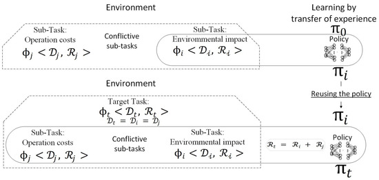
Figure 7.
Schematic approach to transfer learning by reinforcement and reuse of the policy.
As noticed, the trade-off has been approached as a multi-task optimization problem by transferring experience. From now on, to approach the problem, we optimize based on the indices of and , Equations (7) and (8). Consequently, a single agent has the next reward,
The state vector , , (g·Nm), (g·Nm), is the readily biodegradable substrate and (g·Nm). This new state is added because its influence complements the other states in calculating the indexes above (Section 2.1).
In taking this perspective, to achieve the proposed objectives by controlling the states, it is necessary to set up an oxygen reference to reduce without significantly impacting and increments. For this purpose, the actions provided by all the RL agents are three possible increments for the oxygen set point (), , concerning , being (g·Nm): . In addition, the set points of reactors 3 and 4 are and , respectively. As a result, during training, the agent can reach the maximum and minimum oxygen set point values, 0.5 and 6 (g·Nm). For these limits to be respected, the following penalty condition is applied:
As observed, the is smaller the farther the oxygen set pot is from six () or zero (). In addition, minimum is far from the minimum reward, indicating that the penalized policy does not follow a desired strategy.
Once the plant description, the control objectives, the training algorithm, and our state action reward are detailed, it will be easy to identify our agent–environment interaction as shown in Figure 8: At , the agent receives the , and responds with , which is one of the possible increments for , [−0.5 0 0.5] that added to 2 (the initial value) gives the = 2 + , and also and are obtained. At , as a consequence of the set points at t = 0, and a reward value are obtained, and to this feedback, the agent responds by sending , so = + is obtained, and also and are obtained. This interaction is repeated in each episode until the maximum number of time steps t established for training is reached.
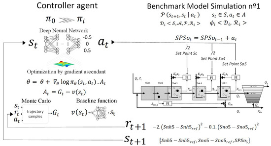
Figure 8.
Control strategy and training approach by the PG algorithm, .
4.4. Deep Neural Network as Policy
The model-free RL benefits from deep neural networks as a function to approximate the parametrized policy . In our case, we used the policy gradient (Section 4) algorithm to update the weights of our deep neural networks until our control objectives are achieved. The setup and structure of these deep neural networks are quite straightforward. Hence, for agents policy, five intermediate fully connected layers with neurons are used, respectively. On the other hand, the policy contains six fully connected layers, with neurons, respectively. As Section 4 discusses, we used the baseline in PG. For this reason, we used a neural network as an approximation function of the baseline function; more precisely, the baseline neural network with three intermediate fully connected layers, composed by 30,30 and 15 neurons, respectively. Furthermore, the baseline neural network contains four fully connected layers, with neurons, respectively.
The policy-DNN and the baseline-NN inputs are the states vector s, the policy-DNN outputs the probability of selecting the action a given a state s, and the output of the baseline network is the baseline value. Furthermore, the policy exploration follows a categorical probability distribution. For this reason, its last layer is a Softmax activation function that gives each neuron the probability of the action, , concerning the state s. This last layer normalizes the input value into an output vector of values that follow a probability distribution, applying the following Softmax function to the input:
where x is the vector values output of the prior layer, is one of our possible increments, , is the probability of select an increment given x, k is the total number of possible increments, , , , is the conditional probability of the increment of given x, and is the prior probability of the increment.
In addition, encountering a set of proper hyper-parameters for training a specific problem is crucial for RL. Although automatically setting the hyper-parameters is an option, we tuned them manually. The configuration of the is as follows: learning rate policy-DNN set to 0.001, learning rate baseline-NN set to 0.01. For , 0.0005 and 0.005 are set, respectively. Furthermore, an adaptive moment estimation (Adam) optimizer was employed.
4.5. Performance during Training
The training of the RL agents was carried out on the : considering ideal sensors and no noise, under dry conditions, with episodes of 14 days and sampling every 15 min, making a total of 1345 RL time steps per episode.
4.5.1. Objectives Evolution
This subsection details the resolution of the sub-tasks along the training and re-training episodes. Therefore, the following metrics are considered: Equation (16) as the integral square error of ammonia in reactor 5 () concerning , Equation (17) as the integral square error of nitrate in reactor 5 () concerning , and Equation (18) as the total aeration energy cost. Each training episode is 14 days of simulation, these 14 days contain 1345 training time steps t.
In order to compare the agents that benefited from the experience, agents and are the same as and , respectively. Nevertheless, and training started without prior knowledge. All the agents are summarized in the following Table 2. Table 2 shows the total number of training episodes, the items on which the reward depends, and the items on which the state depends. The sub-index e indicates that the item is the error concerning its reference.
Table 2.
Agents training by deep reinforcement learning.
In addition, to be clear with the minimization of the sub-task and to benefit from the experience, the training analysis is divided into three fields: the first for agents ; the second for agents ; and the last for agent . Furthermore, to be precise with the evolution of the sub-tasks within the reward throughout the training, Figure 9, Figure 10 and Figure 11 show , , and obtained per episode. Regarding the agents, and (1000 episodes) are yellow lines, and (200 episodes) are red lines, and and are blue lines (2000 episodes).
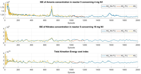
Figure 9.
Evolution of subtasks during training, metrics to assess policy convergence throughout training.
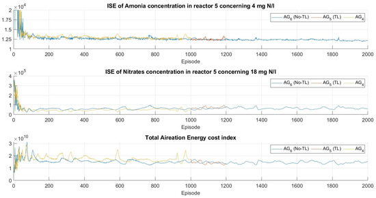
Figure 10.
Evolution of subtasks during training, metrics to assess policy convergence throughout training.
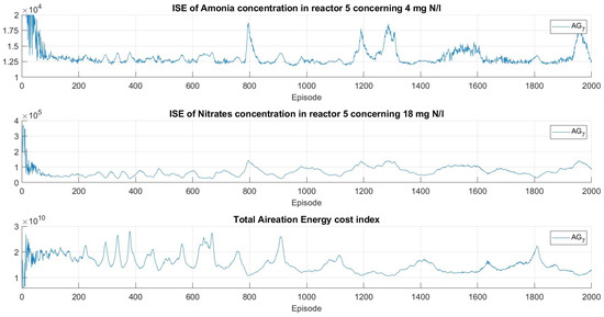
Figure 11.
Evolution of subtasks during training, metrics to assess policy convergence throughout training.
According to Figure 9 and Figure 10, high values at the beginning of the training of the agents that do not take advantage of the experience are shown. Despite the evident continuous decrease in , , do not show an upward trend as expected because of the inverse relationship with . Therefore, all this clarifies the continuous improvement of the decision policies during training. Furthermore, the experience-learning agents continue to learn for the new target stably, without divergence seen at the beginning of the training of the non-experience-learning agents. It is worth noting that, for agents that do not include in their reward, its evolves above those that do include .
Figure 11 shows , whose reward depends on and . The variability of the metrics is higher compared to because , , and in the and indices have different influences, not as direct as in the rewards of .
4.5.2. Oxygen Set-Point Evolution
In this subsection, the evolution of over the episodes is shown to visualize the knowledge transfer. First, Figure 12 and Figure 13 display the () during the first 100 episodes of and , and of and , respectively. Second, Figure 14 and Figure 15 show the divided into groups of 100 consecutive episodes: the last 100 episodes of agents and , the first 100 episodes of agents and (TL agents), and episodes 1000 to 1100 of and . Each line is a throughout the 1345 steps of an episode.
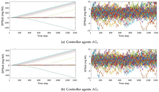
Figure 12.
Oxygen set point of reactor 5 () during exploration in the first 100 training episodes, regular and reduced axe y scale.
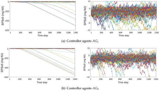
Figure 13.
Oxygen set point of reactor 5 () during exploration in the first 100 training episodes, regular and reduced y axis scale.
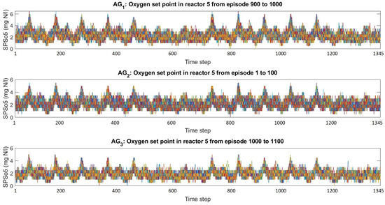
Figure 14.
Controller agents , continuation of learning from the point of view of the obtained with the and the relationship of the dynamics of the with and without knowledge transfer.
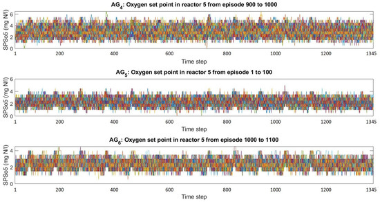
Figure 15.
Controller agents , continuation of learning from the point of view of the obtained with the and the relationship of the dynamics of the with and without knowledge transfer.
The sub-figures of Figure 12 and Figure 13 show the full scale and the −10 to 10 scale. These figures highlight that the scan interval of the first episodes of the four agents is wide, with high contraction violations. Also noteworthy are the very high set points at the start of training, which, as we will see in the following figures, are not repeated due to the effectiveness of penalties.
Figure 14 shows agents . The exploitation of prior knowledge can be explained as follows: the last 100 episodes of show dynamics with no violations of bounds 0 and 6; , which starts its training with the policy of , continues the dynamics of . Moreover, this dynamic has peaks lower than in the case of because includes minimization. Thus, the set points of are comparable to . Basically, this situation is similar for the case of agents , , and in Figure 15. It is important to clarify that the dynamics mentioned above, as will be seen in the results section, are similar to those shown by , which is the element with the highest weight in the rewards of these agents. The policy exploration keeps stable against the added objective and respects the imposed restrictions learned during the previous policy training.
As shown in the previous Figures, the varies roughly. Nevertheless, the filter according to the following equation is added to avoid abrupt changes during the evaluations for validation:
5. Results and Discussion
This section evaluates the agents under the same dry influent training and disturbances, such as the rain and storm influent in and under the . We focus on the differences between the agents trained without and with previous experience. The metrics used are effluent average concentration (), effluent average total nitrogen concentration (), updated aeration energy cost index ( Equation (5)), effluent quality index ( Equation (3)), and operation costs index ( Equation (4)), considering data from the last seven days of simulation according to the BSM1 protocol. The evaluation was performed in MATLAB/Simulink software, 14-day simulations, sampling every 15 min, considering ideal and noiseless sensors, and under the same control strategy as the training (Figure 8).
First, Figure 16 show the evolution of , , , and obtained by the agents over 7–14 days under dry weather conditions. The and involve disturbances: maximums, minimums, and means levels at different intervals. On the other hand, the evolution of follows the concentration on which it directly influences the . Regarding the agents that include the minimization, it is observed that the maximums of are lower than the of agents that do not include . The latter is clearly because the higher the , the higher the cost of .
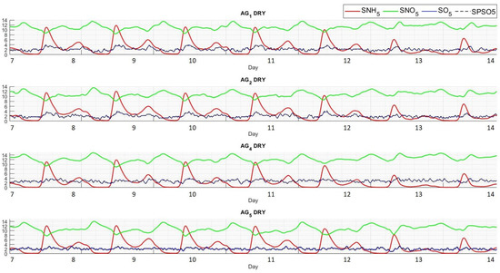
Figure 16.
Controlled concentrations in reactor 5 achieved by along 7 simulation days, including oxygen levels (black discontinued line).
Second, in order to catch the disturbances on the evolution of the levels, Figure 17 () and Figure 18 () show the evolution of , , , and during specific time intervals for dry, rain, and storm weather conditions. According to Figure 17, it is evident that both agents follow the dynamics of the weather disturbances. This situation is similar, although less evident, for agents and in Figure 18. It is noted that the and dynamics reflect the disturbances in the influent. Therefore, following this dynamic means that RL agents give increments that provide peaks at peaks and low values at low levels, as required. In any case, differs between weather conditions due to the different perturbations within the influent. This difference reverberates on , which has an inverse relationship with , specifying that, as the rises, falls and rises. Consequently, the agents respond to this situation with high set points, bringing closer to its reference (18 g·m).
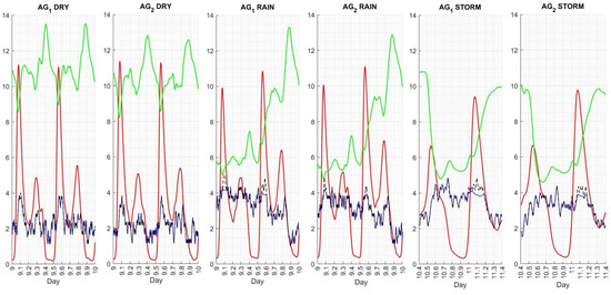
Figure 17.
Controlled concentrations along time in reactor 5 achieved by , including oxygen levels (black discontinued line).
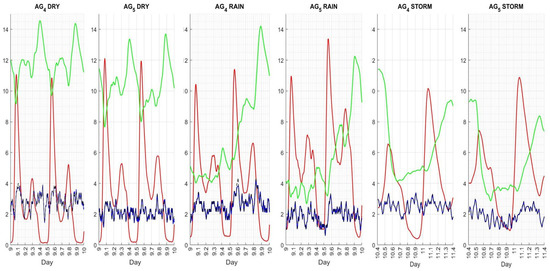
Figure 18.
Controlled concentrations along time in reactor 5 achieved by , including oxygen levels (black discontinued line).
Next, some metrics are analyzed. Figure 19 gives scatters of & under dry, rain, and storm weather conditions for agents. The values are within the limits of ammonia effluent and total nitrogen effluent. On the other hand, considering agents , the (including minimization in its rewards) shows the highest . The inverse relationship between and is efficiently seen. For example, shows lower and high than and . Furthermore, the values obtained are generally grouped into distinct scatter zones due to the different impacts of dry, rain, and storm weather disturbances on plant performance.
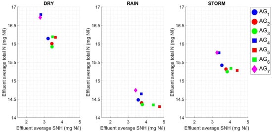
Figure 19.
Average ammonia and total nitrogen concentrations in effluent by a scatter graph for each weather condition.
The numerical values of the above figure are detailed in Table 3. According to Table 3, the difference between the agents that exploited the experience and those that did not is very small. Resultantly, for the and case, the difference in is 0% (DRY), 1.05% (RAIN), and 1.82% (STORM), and the difference in is 0.50% (DRY), 0.34% (RAIN), and 0.45% (STORM), On the other hand, for and , the difference in is 4.91% (DRY), 8.18% (RAIN), and 8.39% (STORM), while the difference in TotN is 0.12% (DRY), 0.34% (RAIN), and 0.39% (STORM). Conversely, the difference between the above and those that did not include the sub-task , , and is significant because of the inverse relation between and . Under these circumstances, aeration energy can be expected to be lower in agents including its minimization. In addition, the table includes , which is the control strategy used by the agents, but with constants = 2 (g·m).
Table 3.
Average ammonia and total nitrogen concentrations in effluent by values for each weather condition.
The following Figure 20 shows the aeration energy cost , a bar chart for each weather condition, highlighting the difference between the agents that do not include and those that include in their rewards, and the similarity between those that do include in their rewards.
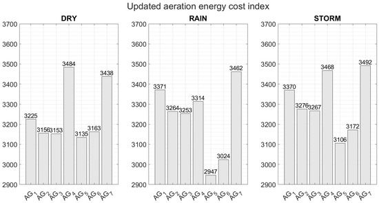
Figure 20.
Aeration energy cost index by bar graph for each weather condition.
Table 4 shows the percentage of operating time in which the and limits were exceeded under DRY, RAIN, and STORM. Much similarity is observed in agents whose reward includes the minimization of aeration energy cost (), and also the highest percentage of violation time. In addition, ammonia violations are higher in RAIN and STORM.
Table 4.
Violations of the maximum effluent total ammonia level (4 mg N/l) and the maximum effluent total nitrogen level (18 mg N/l) limits in percentage (%) of operation time.
Since, in the states of , the agents’ legal limit is present, Table 5 shows the , , and of agents setting (g·m) and (g·m) in its states in order to add a stringent constraint on that concentration. It is observed that, as decreases, also decreases.
Table 5.
Changes in the () reference in the states of the agents .
Alternatively, Figure 21 depicts the evaluation indexes related to environmental impact () and operating cost (). Accordingly, these indexes include , , and , among others, noticed in Section 2. The upper scatter illustrates the values under all weather conditions in order to have a global perspective of the influence of the different weather disturbances on the environmental impact and operating costs. Also, the lower block of scatters presents the disturbances conditions separately. Hereof, for the agents that include in its rewards, the are lower and with their respective consequences on . According to this situation, agents and are the least affected. Regardless, the agent , whose reward was the minimization of and , reveals the best . However, on the other hand, displays high operating costs, except in . Otherwise, in addition to these scatters, numerical results are also detailed in Table 5.
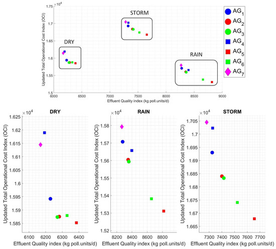
Figure 21.
Effluent quality index and operation cost index by scatter graph for all and each weather condition.
As revealed in Table 6, it is evident that certain effluent quality and operating costs are directly achievable. However, if we want precise objectives, including limits, to be respected, they can also be achieved, as is the case for agents , through TL.
Table 6.
Effluent quality index and operation cost index by value for each weather condition.
As observed, the RL agents achieved the proposed objectives in their simple multi-objective rewards, achieving sub-optimal policies capable of being reused to achieve new objectives. There are no significant differences between the agents trained with and without previous experience, thus highlighting the efficiency of this simple format of reusing policy. Furthermore, the number of episodes required to achieve good results employing transfer learning is considerably smaller.
BSM2
Finally, the obtained agents were validated in the platform: 609-day simulations, sampling every 15 min, considering ideal and noiseless sensors, and under the same control strategy of the training (Figure 8) were considered. The metrics were obtained from days 245–609 and computed using full .
First, Figure 22 shows the evolution of , , , and over days 556 to 562. and involve particular trends but, unlike their peers in the figures’ results, they are closer to zero because the dynamic is not the same as the dynamic. Therefore, the response of the agents is the consequence of being so far from its reference, causing the agent to trigger high to bring the closer to its reference. This situation is similar to the one seen in RAIN and STORM in Figure 18 and Figure 19.
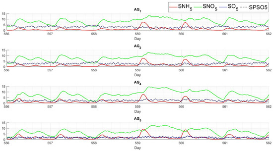
Figure 22.
Controlled concentrations in reactor 5 achieved by along 556-562 days in , including oxygen levels (black discontinued line).
Second, the metrics , , and are detailed in Table 7. Agents that minimize show a lower energy consumption. Consequently, these agents show a high and its respective consequence in . Furthermore, from the general trend of these results, stands out, showing the highest consumption and, of course, the lowest value. In fact, the objective of was to minimize the but not the minimization errors concerning the legal limits.
Table 7.
Average ammonia (mg N/l) and total nitrogen (mg N/l) concentrations in effluent and aeration cost index according to BSM2 protocol.
In fact, from a reinforcement learning context, the transition function of () is different from that of . Consequently, in the evaluation, the state is known but not expected. According to its training, the RL agents respond appropriately to these unexpected states. It is necessary to remark that, despite being evaluated under disturbances and a dynamic not seen during training, the agents provide set point increments that never exceed the restrictions established during training.
6. Conclusions
Due to the complex non-linearity, the relationship between variables, influent disturbances, and uncertainty of the real environment, and, more importantly, the inaccuracy of the mathematical models that approximate it, controlling wastewater treatment processes is challenging. This control problem has motivated researchers to propose methodologies handled by control intelligence. Among them, reinforcement learning is a machine learning methodology that, in addition to having control theory behind it, bases its learning as a human brain would: an iterative trial–error process. A point yet to be resolved in RL is the slow convergence of learning, which makes its applicability computationally inefficient.
In this work, we employed an RL agent as an intelligent controller for this complex oxygen-dependent biological process in WWTPs. The training episodes require high computation costs and time for this complex environment. Necessarily, we used a transfer learning approach between RL agents to make the implementation computationally efficient. More precisely, once an agent has achieved a sub-task, it is re-trained to achieve a new task that turns out to be complementary and a counterpart to the one already achieved. In fact, the most notable difference between agents without and with prior experience is 1.82% for effluent average concentration. To this end, the RL controller can handle the dynamic process without prior knowledge of the dynamic process to perform favorable results, as was demonstrated, achieving the proposed multi-objectives during training and evaluation. Indeed, the evaluation induced the adaptability of RL under different disturbances of the process, despite not training in those unfavorable situations. As an important remark, the RL controllers learned the constraints online and respected them in their evaluation. Therefore, our results are consistent with the motivation to implement model-free reinforcement learning and take advantage of transfer learning.
Another main consideration of the implementation is that, even though the agent has an optimal control theory background, it is simple to define its training elements, especially the design of the reward function, and implement them to approach this control problem, as demonstrated. The deep reinforcement learning methodology emulates the human learning strategy; for this reason, the trial–error training principles can be easily understood by those who are not control specialists.
Author Contributions
Conceptualization, O.A.-R., M.F., R.V., P.V. and S.R.; formal analysis, O.A.-R., M.F., R.V. and S.R.; funding acquisition, M.F. and P.V.; investigation, O.A.-R. and P.V.; methodology, P.V.; project administration, M.F. and P.V.; resources, M.F. and P.V.; software, O.A.-R.; supervision, M.F., R.V. and S.R.; validation, O.A.-R. and P.V.; visualization, O.A.-R.; writing—original draft, O.A.-R.; writing—review and editing, M.F., P.V. and S.R. All authors have read and agreed to the published version of the manuscript.
Funding
This work was supported by projects PID2019-105434RB-C31 and TED2021-129201B-I00 of the Spanish Government and Samuel Solórzano Foundation Project FS/11-2021.
Data Availability Statement
Not applicable.
Conflicts of Interest
The authors declare no conflict of interest.
References
- Li, D.; Zou, M.; Jiang, L. Dissolved oxygen control strategies for water treatment: A review. Water Sci. Technol. 2022, 86, 1444–1466. [Google Scholar] [CrossRef] [PubMed]
- Sheik, A.G.; Tejaswini, E.; Seepana, M.M.; Ambati, S.R.; Meneses, M.; Vilanova, R. Design of Feedback Control Strategies in a Plant-Wide Wastewater Treatment Plant for Simultaneous Evaluation of Economics, Energy Usage, and Removal of Nutrients. Energies 2021, 14, 6386. [Google Scholar] [CrossRef]
- Revollar, S.; Vega, P.; Francisco, M.; Vilanova, R. A hierachical Plant wide operation in wastewater treatment plants: Overall efficiency index control and event-based reference management. In Proceedings of the 2018 22nd International Conference on System Theory, Control and Computing (ICSTCC), Sinaia, Romania, 10–12 October 2018; pp. 201–206, ISSN 2372-1618. [Google Scholar] [CrossRef]
- Vega, P.; Revollar, S.; Francisco, M.; Martín, J. Integration of set point optimization techniques into nonlinear MPC for improving the operation of WWTPs. Comput. Chem. Eng. 2014, 68, 78–95. [Google Scholar] [CrossRef]
- Revollar, S.; Vega, P.; Francisco, M.; Meneses, M.; Vilanova, R. Activated Sludge Process control strategy based on the dynamic analysis of environmental costs. In Proceedings of the 2020 24th International Conference on System Theory, Control and Computing (ICSTCC), Sinaia, Romania, 8–10 October 2020; pp. 576–581, ISSN 2372-1618. [Google Scholar] [CrossRef]
- Sutton, R.S.; Barto, A.G. Reinforcement Learning, Second Edition: An Introduction; MIT Press: Cambridge, MA, USA, 2018. [Google Scholar]
- Bertsekas, D. Reinforcement Learning and Optimal Control; Athena Scientific: Nashua, NH, USA, 2019. [Google Scholar]
- Mousavi, S.S.; Schukat, M.; Howley, E. Deep reinforcement learning: An overview. In Proceedings of the SAI Intelligent Systems Conference (IntelliSys) 2016, London, UK, 21–22 September 2016; pp. 426–440. [Google Scholar]
- Zhang, J.; Kim, J.; O’Donoghue, B.; Boyd, S. Sample Efficient Reinforcement Learning with REINFORCE. Proc. AAAI Conf. Artif. Intell. 2021, 35, 10887–10895. [Google Scholar] [CrossRef]
- Devlin, S.M.; Kudenko, D. Dynamic potential-based reward shaping. In Proceedings of the 11th International Conference on Autonomous Agents and Multiagent Systems, Valencia, Spain, 4–8 June 2012; pp. 433–440. [Google Scholar]
- Harutyunyan, A.; Devlin, S.; Vrancx, P.; Nowé, A. Expressing arbitrary reward functions as potential-based advice. In Proceedings of the AAAI Conference on Artificial Intelligence, Austin, TX, USA, 25–30 January 2015; Volume 29. [Google Scholar]
- Yang, M.; Nachum, O. Representation matters: Offline pretraining for sequential decision making. In Proceedings of the International Conference on Machine Learning. PMLR, Virtual, 18–24 July 2021; pp. 11784–11794. [Google Scholar]
- Hester, T.; Vecerik, M.; Pietquin, O.; Lanctot, M.; Schaul, T.; Piot, B.; Horgan, D.; Quan, J.; Sendonaris, A.; Osband, I.; et al. Deep q-learning from demonstrations. In Proceedings of the AAAI Conference on Artificial Intelligence, Orleans, LA, USA, 2–7 February 2018; Volume 32. [Google Scholar]
- Gupta, A.; Devin, C.; Liu, Y.; Abbeel, P.; Levine, S. Learning invariant feature spaces to transfer skills with reinforcement learning. arXiv 2017, arXiv:1703.02949. [Google Scholar]
- Ammar, H.B.; Taylor, M.E. Reinforcement learning transfer via common subspaces. In Proceedings of the Adaptive and Learning Agents: International Workshop, ALA 2011, Taipei, Taiwan, 2 May 2011; pp. 21–36. [Google Scholar]
- Rusu, A.A.; Rabinowitz, N.C.; Desjardins, G.; Soyer, H.; Kirkpatrick, J.; Kavukcuoglu, K.; Pascanu, R.; Hadsell, R. Progressive neural networks. arXiv 2016, arXiv:1606.04671. [Google Scholar]
- Fernando, C.; Banarse, D.; Blundell, C.; Zwols, Y.; Ha, D.; Rusu, A.A.; Pritzel, A.; Wierstra, D. Pathnet: Evolution channels gradient descent in super neural networks. arXiv 2017, arXiv:1701.08734. [Google Scholar]
- Czarnecki, W.M.; Pascanu, R.; Osindero, S.; Jayakumar, S.; Swirszcz, G.; Jaderberg, M. Distilling policy distillation. In Proceedings of the 22nd International Conference on Artificial Intelligence and Statistics, Naha, Japan, 16–18 April 2019; pp. 1331–1340. [Google Scholar]
- Ross, S.; Gordon, G.; Bagnell, D. A reduction of imitation learning and structured prediction to no-regret online learning. In Proceedings of the Fourteenth International Conference on Artificial Intelligence and Statistics, Ft. Lauderdale, FL, USA, 11–13 April 2011; pp. 627–635. [Google Scholar]
- Dogru, O.; Wieczorek, N.; Velswamy, K.; Ibrahim, F.; Huang, B. Online reinforcement learning for a continuous space system with experimental validation. J. Process Control 2021, 104, 86–100. [Google Scholar] [CrossRef]
- Powell, K.M.; Machalek, D.; Quah, T. Real-time optimization using reinforcement learning. Comput. Chem. Eng. 2020, 143, 107077. [Google Scholar] [CrossRef]
- Faria, R.d.R.; Capron, B.D.O.; Secchi, A.R.; de Souza Jr, M.B. Where Reinforcement Learning Meets Process Control: Review and Guidelines. Processes 2022, 10, 2311. [Google Scholar] [CrossRef]
- Shin, J.; Badgwell, T.A.; Liu, K.H.; Lee, J.H. Reinforcement learning–Overview of recent progress and implications for process control. Comput. Chem. Eng. 2019, 127, 282–294. [Google Scholar] [CrossRef]
- Görges, D. Relations between model predictive control and reinforcement learning. IFAC-PapersOnLine 2017, 50, 4920–4928. [Google Scholar] [CrossRef]
- Corominas, L.; Garrido-Baserba, M.; Villez, K.; Olsson, G.; Cortés, U.; Poch, M. Transforming data into knowledge for improved wastewater treatment operation: A critical review of techniques. Environ. Model. Softw. 2018, 106, 89–103. [Google Scholar] [CrossRef]
- Pisa, I.; Morell, A.; Vilanova, R.; Vicario, J.L. Transfer Learning in Wastewater Treatment Plant Control Design: From Conventional to Long Short-Term Memory-Based Controllers. Sensors 2021, 21, 6315. [Google Scholar] [CrossRef] [PubMed]
- Pisa, I.; Santín, I.; Vicario, J.L.; Morell, A.; Vilanova, R. ANN-Based Soft Sensor to Predict Effluent Violations in Wastewater Treatment Plants. Sensors 2019, 19, 1280. [Google Scholar] [CrossRef] [PubMed]
- Pisa, I.; Santín, I.; López Vicario, J.; Morell, A.; Vilanova, R. A recurrent neural network for wastewater treatment plant effuents’ prediction. In Proceedings of the Actas de las XXXIX Jornadas de Automática, Badajoz, Spain, 5–7 September 2018; pp. 621–628. [Google Scholar] [CrossRef]
- Chen, K.; Wang, H.; Valverde-Pérez, B.; Zhai, S.; Vezzaro, L.; Wang, A. Optimal control towards sustainable wastewater treatment plants based on multi-agent reinforcement learning. Chemosphere 2021, 279, 130498. [Google Scholar] [CrossRef]
- Hernández-del Olmo, F.; Gaudioso, E.; Dormido, R.; Duro, N. Tackling the start-up of a reinforcement learning agent for the control of wastewater treatment plants. Knowl.-Based Syst. 2018, 144, 9–15. [Google Scholar] [CrossRef]
- Jeppsson, U.; Pons, M.N.; Nopens, I.; Alex, J.; Copp, J.; Gernaey, K.; Rosen, C.; Steyer, J.P.; Vanrolleghem, P. Benchmark simulation model no 2: General protocol and exploratory case studies. Water Sci. Technol. 2007, 56, 67–78. [Google Scholar] [CrossRef]
- Alex, J.; Benedetti, L.; Copp, J.; Gernaey, K.V.; Jeppsson, U.; Nopens, I.; Pons, M.N.; Steyer, J.P.; Vanrolleghem, P. Benchmark Simulation Model no.1 (BSM1). In Proceedings of the IWA World Water Congress 2008, Vienna, Austria, 7–12 September 2008. [Google Scholar]
- Ahansazan, B.; Afrashteh, H.; Ahansazan, N.; Ahansazan, Z. Activated sludge process overview. Int. J. Environ. Sci. Dev. 2014, 5, 81. [Google Scholar]
- Gernaey, K.V.; van Loosdrecht, M.C.M.; Henze, M.; Lind, M.; Jørgensen, S.B. Activated sludge wastewater treatment plant modelling and simulation: State of the art. Environ. Model. Softw. 2004, 19, 763–783. [Google Scholar] [CrossRef]
- Santín, I.; Vilanova, R.; Pedret, C.; Barbu, M. New approach for regulation of the internal recirculation flow rate by fuzzy logic in biological wastewater treatments. ISA Trans. 2022, 120, 167–189. [Google Scholar] [CrossRef]
- Revollar, S.; Meneses, M.; Vilanova, R.; Vega, P.; Francisco, M. Quantifying the Benefit of a Dynamic Performance Assessment of WWTP. Processes 2020, 8, 206. [Google Scholar] [CrossRef]
- Revollar, S.; Vilanova, R.; Francisco, M.; Vega, P. PI Dissolved Oxygen control in wastewater treatment plants for plantwide nitrogen removal efficiency. IFAC-PapersOnLine 2018, 51, 450–455. [Google Scholar] [CrossRef]
- Williams, R.J. Simple Statistical Gradient-Following Algorithms for Connectionist Reinforcement Learning. In Reinforcement Learning; Sutton, R.S., Ed.; The Springer International Series in Engineering and Computer Science; Springer US: Boston, MA, USA, 1992; pp. 5–32. [Google Scholar] [CrossRef]
- Agarwal, A.; Kakade, S.M.; Lee, J.D.; Mahajan, G. Optimality and Approximation with Policy Gradient Methods in Markov Decision Processes. In Proceedings of the Thirty Third Conference on Learning Theory, Graz, Austria, 9–12 July 2020; pp. 64–66, ISSN 2640-3498. [Google Scholar]


Disclaimer/Publisher’s Note: The statements, opinions and data contained in all publications are solely those of the individual author(s) and contributor(s) and not of MDPI and/or the editor(s). MDPI and/or the editor(s) disclaim responsibility for any injury to people or property resulting from any ideas, methods, instructions or products referred to in the content. |
© 2023 by the authors. Licensee MDPI, Basel, Switzerland. This article is an open access article distributed under the terms and conditions of the Creative Commons Attribution (CC BY) license (https://creativecommons.org/licenses/by/4.0/).