Article

Intelligent Optimization of Gas Flooding Based on Multi-Objective Approach for Efficient Reservoir Management

1
Research Institute of Petroleum Exploration and Development, PetroChina, Beijing 100083, China
2
CNPC International Hong Kong Limited—Abu Dhabi, Abu Dhabi 999041, United Arab Emirates
3
Shenzhen Branch, China National Offshore Oil Corporation, Shenzhen 518000, China
*
Authors to whom correspondence should be addressed.
Processes 2023, 11(7), 2226; https://doi.org/10.3390/pr11072226
Submission received: 14 June 2023 / Revised: 17 July 2023 / Accepted: 18 July 2023 / Published: 24 July 2023
(This article belongs to the Special Issue Advances in Enhancing Unconventional Oil/Gas Recovery)

Abstract

:
The efficient development of oil reservoirs mainly depends on the comprehensive optimization of the subsurface fluid flow process. As an intelligent analysis technique, artificial intelligence provides a novel solution to multi-objective optimization (MOO) problems. In this study, an intelligent agent model based on the Transformer framework with the assistance of the multi-objective particle swarm optimization (MOPSO) algorithm has been utilized to optimize the gas flooding injection–production parameters in a well pattern in the Middle East. Firstly, 10 types of surveillance data covering 12 years from the target reservoir were gathered to provide a data foundation for model training and analysis. The prediction performance of the Transformer model reflected its higher accuracy compared to traditional reservoir numerical simulation (RNS) and other intelligent methods. The production prediction results based on the Transformer model were 21, 12, and 4 percentage points higher than those of RNS, bagging, and the bi-directional gated recurrent unit (Bi-GRU) in terms of accuracy, and it showed similar trends in the gas–oil ratio (GOR) prediction results. Secondly, the Pareto-based MOPSO algorithm was utilized to fulfil the two contradictory objectives of maximizing oil production and minimizing GOR simultaneously. After 10,000 iterations, the optimal injection–production parameters were proposed based on the generated Pareto frontier. To validate the feasibility and superiority of the developed approach, the development effects of three injection–production schemes were predicted in the intelligent agent model. In the next 400 days of production, the cumulative oil production increased by 25.3% compared to the average distribution method and 12.7% compared to the reservoir engineering method, while GOR was reduced by 27.1% and 15.3%, respectively. The results show that MOPSO results in a strategy that more appropriately optimizes oil production and GOR compared to some previous efforts published in the literature. The injection–production parameter optimization method based on the intelligent agent model and MOPSO algorithm can help decision makers to update the conservative development strategy and improve the development effect.

1. Introduction

Highly uncertain and disputable parameters are one of the main concerns in the process of reservoir management and decision making. Influenced by reservoir heterogeneity and unreasonable injection–production parameter combinations, the abundant remaining oil is difficult to drive and becomes more dispersed. Therefore, the original development plan is unable to achieve satisfactory performance. To improve the effectiveness of the development plan, the injectors are adjusted to reduce the inefficient or ineffective injection volume. Reasonable optimization helps to increase the oil rate and control the risk warning parameters, such as the water cut (WCT) and GOR. Therefore, a reasonable optimization strategy is an effective strategy to improve reservoir development.
To optimize the overall structure, improve the final recovery factor, and reduce development risks, the need to optimize the injection–production parameters has been proposed. In the middle and later stages of development, the existing parameters face challenges, such as unclear effectiveness and high development risks. Specifically, unreasonable parameters lead to fluid intrusion. On the one hand, this renders the remaining oil more dispersed, which restricts the development effect; on the other hand, the unreasonable adjustment of the injected fluid can easily lead to ineffective circulation and even result in high-risk producers.
Water/gas injection is an effective displacement measure that can restore the reservoir pressure and achieve a higher recovery factor. Therefore, the choice of injection fluid has a strong impact on oil recovery. Khormali [1] used two different types of formation water to simulate the effects of reservoir pressure, temperature, injection water, and pairing on inorganic salt formation, and they proposed a reasonable ratio of injection water to formation water, guiding the rational selection of optimized injection–production parameters.
One of the essential tasks in achieving efficient reservoir development is to obtain the best combination of injection–production parameters quickly and accurately. There are four commonly used methods (Table 1). The first method is to distribute the total production and injection volume to all producers and injectors evenly [2], which is simple but carries many disadvantages. Firstly, for strongly heterogeneous reservoirs, the development effectiveness varies greatly between regions. Therefore, it is difficult for a simple uniform distribution to reflect the actual conditions of the reservoir. Secondly, due to the irregular distribution of the remaining oil, it is difficult to achieve efficient potential tapping in this way.
The second method is to allocate the parameters according to the reservoir characteristics. An [3] selected the pore volume and remaining geological reserves as the distribution index. Because the index has a certain physical meaning, this method helps to achieve efficient potential tapping. Moreover, it can effectively suppress the risk of water and gas invasion, ensuring the injection effectiveness simultaneously. However, this method also has certain limitations. First, the appropriateness of the allocation has a strong relationship with the accuracy of the RNS model. Because many basic data and complicated historical fitting are required, it is difficult to reach high accuracy and ensure authenticity. Secondly, the selection of indicators does not consider specific optimization objectives, so it is difficult to determine whether the proposed strategy is the optimal solution.
The third method is based on RNS and statistical methods, represented by the response surface methodology (RSM) [4]. The RSM helps to obtain the global optimal scheme. Specifically, the RSM fits complex unknown functional relationships with relatively simple first-order or second-order polynomial models, which reduces the computational complexity. Secondly, compared with the orthogonal experimental design, the RSM can continuously analyze all levels of the experiment in the process of optimization, which greatly improves the feasibility of the model. Based on the RNS and RSM, Kang [5] designed a optimization process for the EOR and many steam and gas push (SAGP) parameters (including the injection gas type, injection time, injection gas mol, and volume). Based on the results, the best combination of all factors was effectively determined, providing a good reference for the improvement of reservoir development efficiency. Based on a higher-order polynomial equation, Wantawinj [6,7] established a simpler and more efficient reservoir agent model using the RSM. Compared with the commonly used quadratic form model, this method shows higher accuracy in the direction of shale reservoir evaluation, fracture characterization, and production prediction. However, the application of the RSM is limited due to the slow computational speed of RNS models. In addition, if the range of experimental points is not selected properly, it will be difficult to obtain good optimization results. Therefore, reasonable experimental factors and corresponding levels should be determined before using the RSM.
The forth method is to optimize the parameters by defining the objective function and embedding the optimization algorithm into the RNS model. The extreme optimal value of the objective function is searched through iterations. This method can consider specific objectives, further improving the relevance of optimization. Taking the Net Present Value (NPV) as the objective function, Sarma [8] explored a new water injection optimization strategy using the optimal control algorithm and verified it using the black oil simulation model, which showed good application results. In addition, apart from the NPV [9,10,11], different objective functions can be considered, such as GOR, WCT, and so on, depending on the specific situation. However, it is still difficult to overcome some shortcomings, such as the time-consuming process. On the other hand, commonly used optimization algorithms such as particle swarm optimization (PSO) [12,13] and genetic algorithm (GA) [14,15,16,17] mainly focus on a single objective, which limits the scope of application in the oilfield. Instead, two or more objective functions should be taken into consideration.
Many studies have contributed to the MOO problem [18,19] in terms of on-site requirements, which can be summarized into three aspects. The first is to assign weighting factors to each objective, converting multiple objectives into a single function. In this way, a single objective optimization technique such PSO or GA can be utilized to seek the optimal results. This method is easy to understand but it is unable to provide an effective solution for MOO, where the relative importance is not clear. The second is to consider the relative importance of the objective function, called lexicographic optimization. This type of method is suitable for problems where different objective functions have different priorities. However, it cannot provide a comparative analysis of the tradeoffs between different functions. To address the shortcomings of the above methods, the Pareto-based method is favored because it can provide decision makers with a tradeoff analysis [20]. The basic idea is to iterate and plot the Pareto frontier by calculating the fitness, which is suitable for problems where the importance of different objectives is unclear.
Table 1. Comparison of conventional injection–production parameter optimization methods based on RNS.
MethodDescriptionAdvantagesLimitations
Uniform divisionDivided by uniform conditions [2]1. Simple.
2. Suitable for weakly heterogeneous reservoirs.
1. Lack of physical basis.
2. Extremely poor applicability in highly heterogeneous reservoirs.
Proportional divisionDivided by reservoir properties [3]1. Considers the actual conditions of the reservoir to a certain extent.
2. Suppresses the risk of water and gas invasion effectively.
1. Relatively dependent on the accuracy of RNS models.
2. Difficult to determine whether the result is the optimal solution.
Divided according to statistical methods [5,6,7]1. The main factors of the reservoir could be obtained.
2. The computational complexity is reduced.
3. Can continuously analyze various experimental levels.
1. Constrained by the calculation speed of RNS.
2. The optimization results rely heavily on the selection of experimental point ranges.
Divided using iterative optimization [21,22,23]1. Considers specific objectives, improving the relevance.
2. Obtains unique optimal result of the objective function.
1. Relatively dependent on the accuracy of RNS models.
2. Only one objective is considered mainly.
Pareto-based optimization algorithms are often embedded in population-based evolutionary algorithms, such as the non-dominated sorting genetic algorithm II (NSGA-II) and MOPSO [19,24,25,26,27,28]. Wang [29] designed a fracturing optimization scheme based on the least squares support vector regression (LSSVR) and NSGA-II. They applied the proposed framework to a shale gas reservoir, shortening the optimization time and improving the accuracy, and the work provides a reference for subsequent fracturing operations. Desbordes [30] proposed a production optimization framework integrating three evolutionary algorithms, namely NSGAII, MOPSO, and the multi-objective evolutionary algorithm based on decomposition (MOEA/D). Due to the elimination of the population reinitialization step, the method can achieve relatively high fitness with a lower computational cost. Due to the limitations of RNS [31], there is an urgent need for a method that can compensate for its shortcomings in various aspects [32].
Big data and artificial intelligence (AI) technology surpass the traditional physical-driven research thinking and deeply explore the logical relationships existing within data [33]. AI has the advantages of simplicity, high speeds, and high computational accuracy because it can learn the inherent nonlinear mapping relationships of data directly. Reservoir engineers can store and manage data and conduct in-depth mining and analysis to propose development plans. Thanks to advances in computing power and the iterative updating of algorithms, AI has also become a key technology for the intelligent exploration of oilfields. These applications mainly focus on PVT prediction [34,35,36], missing value regression [37], well location prediction [38,39], history matching [40,41,42], and production prediction [43,44,45,46,47,48]. Many studies indicate that AI technology can improve the efficiency and economic benefits. Therefore, AI technology is expected to alleviate the shortcomings of RNS and play a greater role in oil exploration and development.
Transformer is a neural network that processes sequential data based on a self-attention mechanism. The core of Transformer is the attention mechanism; similar to human selective visual attention, it can learn information that is more critical to the current task goal from a variety of information, which enhances the time series modeling ability. With this ability, Transformer has achieved remarkable success in natural language processing and computer vision, demonstrating its powerful time series modeling capabilities. Guo [49] and Bai [50] predicted future traffic flows based on an attention-based graph convolutional network. The prediction results showed that the attention-based model had higher accuracy compared to traditional neural networks. Wang [51] proposed a short-term load forecasting method based on an attention mechanism and the bi-directional long short-term memory (Bi-LSTM) neural network to update data, assign weights, and perform model training and prediction, respectively. After comparing the prediction results of actual datasets, the results showed that the model with the attention mechanism had a lower calculation error, indicating the superiority of the attention mechanism. Similarly, Liu [52] combined an attention mechanism and the Bi-GRU neural network to optimize the hypertext transfer protocol’s security. Niu [53] used an attention mechanism to predict wind power, achieving good results. In the petroleum industry, attention mechanisms have also been applied in production forecasting. Therefore, compared with existing deep learning methods, attention-based methods significantly improve the prediction accuracy.
This article establishes a workflow for injection–production parameters’ intelligent optimization considering the multi-objective tasks of the oilfield. The basic processes include establishing an attention-based Transformer intelligent agent model, to perform multi-objective optimization tasks via the Pareto-based population evolutionary optimization algorithm. This article is divided into the following sections. In Section 2, we introduce the methodology of the Transformer model and MOPSO algorithm. Section 3 introduces the multiple objectives, the basic information of the target reservoir, the data preprocessing process, and the architecture and evaluation criteria. In Section 4, the proposed method is evaluated and compared with other methods. The discussion and conclusions are given in Section 5 and Section 6.

2. Methodology

2.1. Transformer

Currently, many supervised learning algorithms can be used to build intelligent agent models. These methods can be mainly divided into classification algorithms and regression algorithms, represented by decision tree, support vector machine (SVM), random forest (RF), etc. Because of their simple structures and fast speeds, classification algorithms are also widely used in time series prediction. However, since the actual data are mostly non-stationary, the simple structures of classification algorithms do not have the ability to learn complex data. Therefore, this limits their application in time series prediction.
As another powerful tool in time series prediction, artificial neural networks (ANN) are widely used to interpret and predict times series data. The most commonly used deep learning methods for the processing of time series currently include the recurrent neural network (RNN) and its variants, such as long short-term memory (LSTM), the gated recurrent unit (GRU), Bi-LSTM, Bi-GRU, and so on. The RNN is a type of neural network structure aimed at processing time series. The unique connections between hidden layers in the RNN form a directed loop, which enables it to process time series well. As with fully connected neural networks, the simplest RNN consists of three parts: an input layer, hidden layer, and output layer. The value of the hidden layer in the RNN depends not only on the current input x t but also the value of the previous hidden layer h t 1 . The value of the previous hidden layer h t 1 is determined by the input x t 2 and the previous hidden layer h t 2 . In other words, in an ideal situation, its hidden layer can store information for a long time.
o ( t ) = g ( V h ( t ) + b o )
h ( t ) = f ( U x ( t ) + W h ( t 1 ) + b h )
where x ( t ) represents the input vector at time t; o ( t ) represents the output vector; h ( t 1 ) is the hidden cell state at time t − 1; b o and b h are the bias vectors; g ( ) and f ( ) are the activation functions; U , W , V are the weight matrices used for input–hidden connections, hidden–hidden connections, and hidden–output connections, respectively, with the same weight values for the same types of weight connection. L shown in Figure 1 is the loss function, and y is the label of the training set.
To update the RNN weights with the optimal U , W , V , the partial derivatives of the loss function for the three weight matrices are as shown below:
L V = t = 1 n   L ( t ) o ( t ) o ( t ) V
L ( t ) W = k = 0 t   L ( t ) o ( t ) o ( t ) h ( t ) j = k + 1 t   h ( j ) h ( j 1 ) h ( k ) W
L ( t ) U = k = 0 t   L ( t ) o ( t ) o ( t ) h ( t ) j = k + 1 t   h ( j ) h ( j 1 ) h ( k ) U
From Equations (3)–(5), it can be seen that there is no time dependency problem for partial derivatives of V ; however, for U and W , due to the long-term dependence of the time series, h ( t ) will propagate forward with the time series. Due to the gradient vanishing and the explosive linearity of the RNN, its prediction performance is average when processing long sequence data.
To alleviate the gradient vanishing/exploding problem of RNN models, a series of variants have gradually emerged. Information in neural networks represented by LSTM [54] and GRU [55] is transmitted unidirectionally, and only past information can be utilized, without the use of future information. The emergence of bi-directional neural networks, such as Bi-LSTM [46,56] and Bi-GRU [57], has made it possible to consider both past and future information simultaneously. Bi-LSTM connects the two hidden layers of LSTM to the output layer. In this structure, both previous and future information can be utilized at the output layer and this can significantly improve the model performance. However, when using the RNN to process a vector sequence, it requires a “local encoding” of the sequence. Therefore, the RNN has a short-distance dependency and it lacks parallel processing capabilities.
Transformer consists of encoder and decoder stacks. The encoder and decoder of Transformer are both composed of n identical layers [58]. Each encoder layer has two sub-layers, consisting of a multi-head self-attention mechanism and feed forward neural network (FFNN). Each decoder layer has three sub-layers, consisting of a multi-head self-attention mechanism, multi-head attention over the output of the encoder stack, and FFNN. The attention mechanism is the core of Transformer. It indicates the importance of other tags in the input to the encoding of a given tag. The attention mechanism can solve the two problems of the RNN and its variants mentioned above. In response to the difficulty of obtaining long-term dependencies for the RNN and its variants, there is no concept of distance when calculating the attention score. The attention score of each unit and the current unit is independent of their distances, so it can avoid the problem of difficult-to-obtain long-distance dependencies. Transformer can calculate the attention score in parallel to obtain the context vector (Figure 2).
Specifically, we create three randomly initialized training parameter matrices, W Q , W K , and W V   first, and we multiply the encoder input vectors to obtain the corresponding matrices Q , K , and V . Then, we calculate the attention score of each input variable and other units in the data. The attention score represents the degree to which attention is focused on other parts during encoding, and it is calculated by the dot-product of Q and K . Secondly, dividing the score by the square root of the matrix K dimension helps to achieve more stable convergence in training. Subsequently, a SoftMax function is applied to obtain the weights of the values, and each SoftMax value is multiplied. Finally, we add the weighted value vectors together as the corresponding output vectors in the self-attention layer. After the vectors are correlated with each other in the self-attention layer, the corresponding vectors are transferred to the FFNN layer. In the FFNN layer, each link has no correlation, so the FFNN layer can parallelize each input variable. The matrix of output can be computed as in the formula below:
Attention   ( Q , K , V ) = softmax   Q K T d k V
where d k denotes the queries and keys of the dimension.
Multi-head attention is an improvement of the self-attention mechanism (Figure 3). It enhances the model’s ability to focus on various positions by randomly initializing multiple Q / K / V matrices and allows the self-attention layer to have a greater representation space. The specific method is to multiply the calculated multiple output matrices by an additional weight matrix, to obtain information that is the same size as the original and captures all attention heads.
In addition, each self-attention and FFNN layer is linked through a residual and then subjected to layer normalization operation. Furthermore, to read the position information of each piece of data, Transformer adds a position encoding to the input embedding and the final output vector. The calculation formula for the position encoding is as follows:
P E ( p o s , 2 i ) = sin   p o s / 10,000 2 i / d model
P E ( p o s , 2 i + 1 ) = cos   p o s / 10,000 2 i / d model
where p o s is the position and i is the dimension.
Transformer introduces multi-head attention and self-attention modules to first “self-associate” the source and target sequences, enriching the information contained in the embedded representations of the source and target sequences themselves. Furthermore, the subsequent FFNN layers also enhance the model’s expressive and parallel computing capabilities. Therefore, it establishes a good theoretical basis for the subsequent establishment of the intelligent agent model.

2.2. MOPSO

MOO problems are mainly based on multiple conflicting objective functions. Therefore, the optimal solution obtained for a certain goal will not consider other goals in the optimal value and may even lead to degradation. The traditional MOO methods include the weighted sum method, constraint method, objective programming method, distance function method, minimax method, etc. Most of these methods decompose the problem into a single objective problem, relying on different strategies, and single objective algorithms are used to achieve optimization. Due to the reliance on prior knowledge and the inability to select the optimal solution based on different needs, the above methods are not feasible in certain contexts. For example, when MOO problems exhibit complex characteristics such as nonlinearity and high dimensionality, traditional methods are not able to achieve good results.
In recent years, evolutionary algorithms have enabled many breakthrough research achievements in the field of combinatorial and numerical optimization. PSO is an evolutionary algorithm inspired by the foraging behavior of bird populations in nature [27]. Due to its advantages, such as simple implementation, an efficient search, and fast convergence, it has been widely applied in various experimental tests and on-site practical applications.
As an evolutionary version of PSO, MOPSO is currently a popular method [19]. In MOPSO, the individual’s position is treated as the solution to an optimization problem, ignoring the individual’s mass and volume. The main principle is to continuously update the information exchange between individuals in the group and the optimal individual. Moreover, the entire group of individuals is guided to converge towards the optimal individual, retaining their own diversity information.
The update particles are obtained through the organic combination of population history optimal particles and individual history optimal particles. The velocity v i g + 1 of particle i at the next moment is determined by the current velocity v i g , its own optimal position X i , p b e s t g , and global optimal position X i , g b e s t g , which are jointly determined. After updating, the speed changes from the current position X i g to a new position X i g + 1 . As the iteration continues, the entire particle swarm, under the leadership of the leader, completes the search for the optimal solution. The formula is shown below:
X i g + 1 = X i g + v i g + 1 , i N p   and   g N g
v i g + 1 = ω I v i g + ω c R 1 X i , p b e s t g X i g + ω s R 2 X i , g b e s t g X i g
The final visual solution of the MOO problem utilizes the Pareto concept. Pareto optimality refers to an ideal state of resource allocation. In the parameter space S , there is a variable Y , and if there is no variable Y in S that makes all the corresponding objective function values better than the corresponding objective function values, then Y is called the Pareto optimal solution of the objective function, also known as the non-inferior solution. Multi-objective optimization problems have more than one non-inferior solution, and the set composed of all non-inferior solutions is called the non-inferior solution set. The non-inferior solution set is mapped by the objective function to form the Pareto optimal frontier or Pareto frontier surface of the problem. For a problem with two objectives, the Pareto optimal frontier is generally a line.

3. Case Study

3.1. Basic Information of Target Reservoir

Our target is a typical carbonate reservoir in the Middle East, with an anticline reservoir morphology and an initial reservoir pressure of 4425 psi. According to the tectonics of the reservoir, it can be divided into two blocks: the crest area and the flank area. The crest area is mainly developed by injecting miscible gas, and the flank area is mainly developed by WAG. This paper focuses on the crest area. The porosity range is 5–25%, and the permeability ranges from 1.3 to 6.3 mD. Lower permeability is attributed to the blocking of the primary intergranular pore system caused by diagenesis. The specific fluid and reservoir physical parameters are shown in Table 2.
Carbonate reservoirs in the Middle East are mainly composed of porous bioclastic limestone with low permeability, making them very different from fractured-cavity carbonate reservoirs. The micropore structure of a carbonate reservoir is complex, the heterogeneity is strong, and the interlayer and thief layer are generally developed. The reservoir has combinations of platform–edge and reef–shoal, with various types of porous spaces, mainly intergranular pores, while also developing intracrystalline pores, intergranular dissolved pores, intergranular pores, and cavity pores. Such reservoirs are complex and diverse, differing markedly in geologic features and development modes. Therefore, efficient gas injection development is hindered by several challenges.
The crest area injects miscible gas through 11 reverse five-point well patterns, including 18 producers and 11 injectors, with a well spacing of 4100 ft. All wells are completed with 6-inch horizontal wells and open hole completion, with an average horizontal well length of approximately 4000 ft. According to the development plan, as of 2006, the sustainable production amounts to 60 Mbd/day, with a target injection rate of 100 MMscf/d.

3.2. Multi-Objective Function

Due to the presence of a gas cap, the GOR in the crest area continues to rise. While the number of wells opened remains stable, the regional production capacity continues to decline, making it difficult to achieve stable production of 60 Mbd/day. The average GOR of a single well in the reservoir is 1900–2500 scf/bbl. Since the comprehensive transition to WAG development in 2019, the GOR has not significantly decreased. Some wells have approached the shut-in targets set by resource countries, so efficient development is hindered by several challenges.
The MOPSO algorithm is utilized to mathematically define an objective function for a series of objectives in this paper. The final objective function F ( x ) is also called the fitness function. In view of the difficulties in stabilizing the oil production and controlling the GOR in the development of the top area, this paper defines the fitness function as below:
F ( x ) = e x p   Q B R F d , k S n G O R B R F d , k S n + 1
Q and G O R represent the oil production and GOR calculated by the intelligent agent model. The exponential function is used to increase the sensitivity of the objective function. The larger the objective function value, the higher the gas production and the lower the GOR.
An increase in the gas injection volume will increase production, but it will also correspondingly increase the costs. Taking the P-39 well pattern as an example, we first calculate the historical average gas injection rate (GIR) of adjacent wells, as shown in Table 3, and to make the iterative simulation values more realistic, this article adds a constraint on the gas injection volume, as in Equation (12).
1 4 G I R n 50,000   M s c f / d
In this paper, G I R n represents the gas injection rate of the n -th injector.

3.3. Model Training and Data Preprocessing

To establish a high-precision intelligent agent model, 8 types of real parameters of the reservoir were collected from 2006 onwards, including the gas injection volume and injection pressure of 4 adjacent injectors. The output characteristics are the production and GOR. It is worth mentioning that the shut-in state and choke size have a strong improvement effect on oil production and GOR, but they are strongly influenced by human factors. Therefore, to ensure the theoretical authenticity of the model, this article does not consider these two characteristics.
There are four injectors around P-39, namely I-14, I-40, I-74, and I-19. The collected dynamic data cover a range of 4500 days. The relevant characteristic curves of the well group are shown in Figure 4. The heat map between variables is shown in Figure 5.
To improve the quality of the dataset, we sequentially perform data preprocessing steps such as data standardization and data splitting. Due to the different sources of sample features and measurement units, the scales vary greatly, so it is necessary to standardize the sample and convert the features of each dimension into the same value range. Standardized processing can not only reduce the impact of manual intervention in parameter adjustment but also improve the convergence speed of the model. This article introduces a minimum–maximum scaler to normalize the historical dynamic data, and the specific formula is as follows:
x nor   = x i m i n x i m a x x i m i n x i
where x nor   is the input variable after normalization.
The data used in this study are divided into a training set and a testing set, with a ratio of 9:1. The data from the first 4000 days are used as a training set to train the model. The data from the last 500 days are used as a test set to evaluate the prediction performance.

3.4. Model Structure and Evaluation Criterion

The parameter settings involved in the process of building the intelligent agent model based on the Transformer algorithm are shown in Table 4.
In addition, Table 5 lists the hyperparameters of the MOPSO algorithm. The population size is 300, which means that there are 300 particles in each generation that need to be optimized. The iteration number is 10,000, and the inertia weight is 0.7. The individual confidence factor and group confidence factor are both 2.0.
After the prediction, the model needs to be evaluated through statistical evaluation indicators. This paper uses three commonly used error evaluation criteria to study the accuracy of the model results: the root mean square error (RMSE), mean absolute error (MAE), and median absolute error (MedAE). The formulas are as follows:
R M S E = 1 n i = 1 n   y i y ^ i 2
M A E = 1 n i = 1 n   y i y ^ i
M e d A E = M e d i a n   y 1 y ^ 1 , , y n y ^ n
where y i is the i -th actual value, y ^ i is the i -th predicted value, and n is the number of samples in question. y ¯ i is the average actual value of the sample.
To better compare the performance between algorithms, another criterion named accuracy is defined as follows:
A c c u r a c y = 1 1 n i = 1 n   y ^ i y i y i

4. Experimental Results

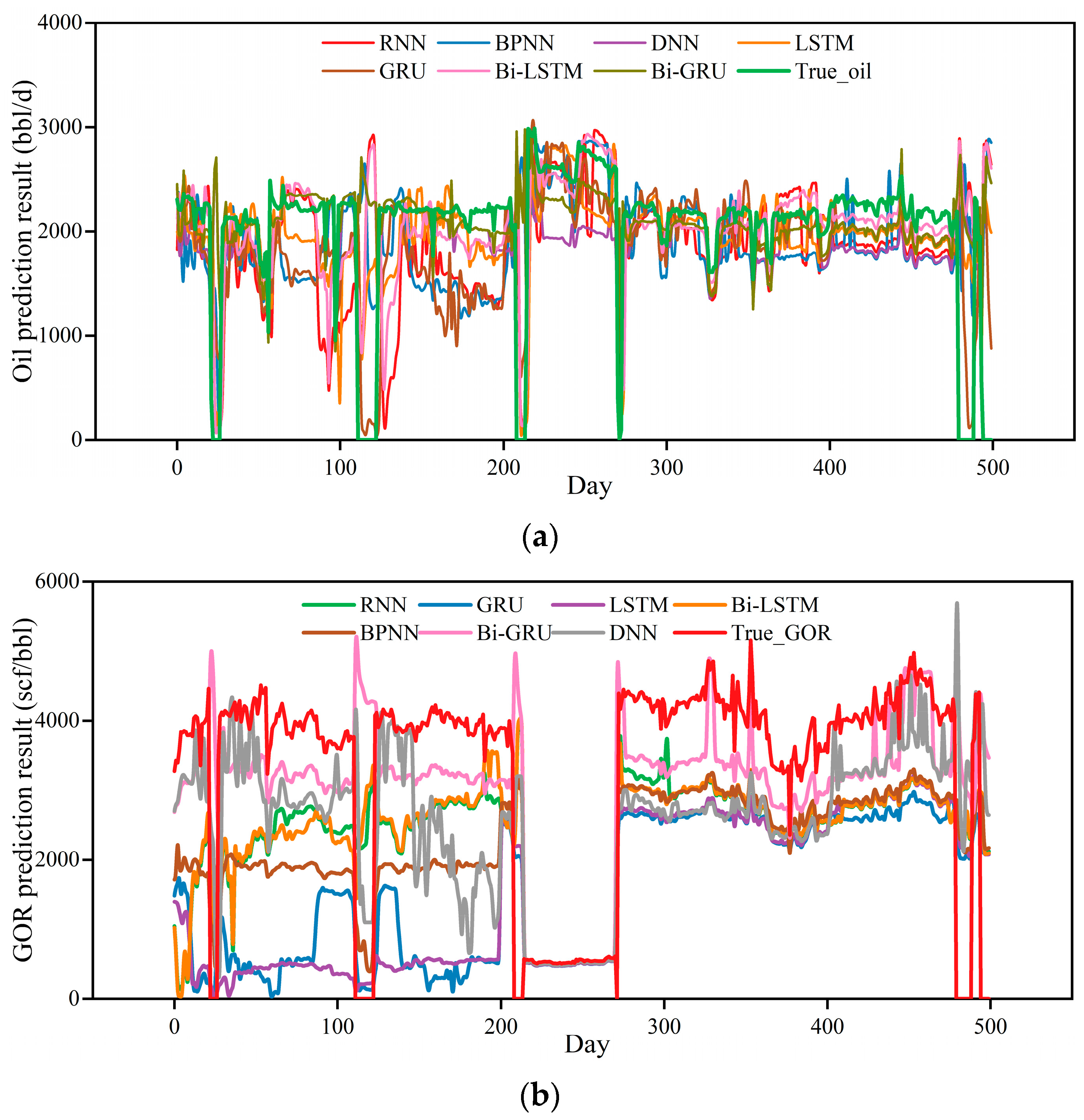
4.1. Performance in Prediction of Production and GOR

Different algorithms are used to predict the production and GOR of the P-39 well, and the ability of the different algorithms to capture information in dynamic prediction is compared. The first is the temporal prediction ability of representative machine learning algorithms. From the prediction results, the machine learning algorithm-based model is not sensitive to changes in time series data, and it yields an almost smooth straight line, with only significant changes occurring at some points (Figure 6). Secondly, in the first 200 days of prediction, the bagging algorithm and RF algorithm are relatively closer to the real data in production and GOR prediction, but the error gradually increases in the later stage. Thirdly, there are fluctuations in production and GOR between 200 and 270 days; however, the machine learning algorithms are unable to capture this trend.
Next, we performed the temporal prediction ability comparison of the neural network algorithms represented by RNN, GRU, LSTM, Bi-LSTM, etc. From the prediction results (Figure 7), the RNN algorithm and its variants are more sensitive to time series data compared with machine learning algorithms. The prediction results have significant fluctuations, similar to the true data, indicating a preliminary trend of capturing time series information. However, due to the difficulty in obtaining long-term dependencies, in the mid- to late stages of prediction, the effectiveness decreases.
By comparing the production and GOR prediction results of common neural network algorithms, we have captured the following information. Firstly, from the overall trend, the deep learning prediction results are more sensitive to time series, reflected in the large fluctuations in production and GOR. Secondly, the GOR prediction trends of Bi-GRU are more closely aligned with the true data; from the statistical error results in GOR prediction (Figure 8b), the RMSE, MAE, and MedAE of Bi-GRU are reduced by 10%, 30%, and 41%, respectively, compared to the RNN. This indicates that the Bi-GRU [55] methods have alleviated the limitations of the RNN.
The error comparison of common algorithms is shown in Figure 8. From the perspective of the production prediction performance, bagging, RF, GRU, Bi-GRU, and Bi-LSTM perform well in terms of the error criteria; the above algorithms perform better than other algorithms in MedAE especially, indicating that such algorithms have better robustness in production prediction. However, in the process of predicting GOR, the prediction error of the AI methods fluctuates greatly. At present, the bagging, AdaBoost, RNN, and Bi-GRU algorithms perform well in terms of the error criteria. Therefore, combining the prediction results of the two development indicators, the bagging and Bi-GRU algorithms have higher accuracy and will be discussed with the Transformer model further.
Finally, the prediction comparison regarding RNS, bagging, Bi-GRU, and Transformer was performed. The prediction results of the Transformer model were compared with those of the commonly used and highly accurate Bi-GRU algorithm. The comparison of the GOR prediction results showed that, compared to Bi-GRU, the RMSE, MAE, and MedAE of the Transformer algorithm were reduced by 28%, 42%, and 78%, respectively, while the accuracy increased by 9%. From the prediction results (Figure 9), the Transformer model [58] is mostly sensitive to time series data and shows better prediction performance throughout the entire prediction stage compared with bagging and Bi-GRU, which, to some extent, alleviates the problem of the traditional RNN being unable to obtain long-term dependencies (Figure 10).
Next, the differences in computational time between different methods were compared. The RNS methods and all intelligent algorithms were executed on professional workstations; the main specifications were as follows: 2 × Intel® Xeon (R) Gold 6230 CPUs @ 2.10 GHz, 256 GB DDR4 memory, and an NVIDIA RTX A5000 graphics card with 24 GB GPU memory. From Table 6, the computation time of RNS was 4600 s, while the computation time of the intelligent algorithms was significantly reduced. The Transformer algorithm has the lowest time consumption, reflecting the parallel computing ability of the attention mechanism.
In conclusion, compared with other methods, the intelligent agent model based on the Transformer model has higher accuracy and a faster computing speed, which can lay the foundation for further injection–production optimization.

4.2. Iteration Result of MOPSO

This section considers the integration of the MOPSO algorithm based on the agent model to find the optimization scheme for the P-39, I-14, I-40, I-74, and I-19 wells. The MOO fitness function integrating production and GOR is defined in Section 3.2, with the aim of finding the optimal solution to achieve both high production and low GOR. Moreover, the required hyperparameters in the MOPSO algorithm are given in Section 3.4.
After 10,000 iterations, the fitness curve and optimal particles of each generation are as shown in Figure 11. Each particle represents the composite pattern of the injection amount and the prediction effect. The horizontal axis represents oil production, and the vertical axis represents the GOR. From the change curve of the fitness function, the fitness gradually increased within 10,000 iterations and became stable in the later period, indicating that the update of the non-dominated solution did not occur within the chosen number of iterations.
According to the above results, the Pareto frontier can be determined. From Figure 12, the Pareto frontier can be divided into three parts, with the curves in part 2 being steeper than those in other parts, indicating that as the oil production increases, the GOR will significantly increase. In parts 1 and 3, the curve is relatively flat, indicating that the GOR is not sensitive to an increase in oil production. Therefore, based on the Pareto frontier, the injection method can be dynamically adjusted on-site. When the reservoir development target is high production, the injection method of particles corresponding to the maximum production rate can be selected. When the production well faces a high GOR, the injection mode corresponding to the minimum GOR can be selected.
Moreover, three optimization schemes are proposed for the P-39 well pattern. Firstly, the average allocation method is proposed based on the target injection volume (50,000 Mscf/d). Secondly, from the perspective of reservoir engineering, the remaining geological reserves in the plane distribution of each well in the simulation model are allocated. Finally, the iterative results proposed in this article are utilized to predict the performance. Then, based on the agent model, the development effects of different injection methods are predicted. The comparison of the injection and production parameters for different schemes is shown in Table 7.
The prediction results of the intelligent agent model are shown in Figure 13. The results indicate that in the next 400 days of production, the average method will face the risk of a production reduction and increasing GOR, which are caused by unreasonable injection parameters. The reservoir engineering method does not have significant production fluctuations, but the development effect needs to be further improved. The method proposed in this article results in higher production and lower GOR. In the next 400 days of production, the cumulative oil production will increase by 25.3% compared to the average distribution method and 12.7% compared to the reservoir method; GOR is reduced by 27.1% and 15.3%, respectively. The method proposed in this article helps to consider the actual situation and find the best injection production plan, which can not only ensure a production increase but also reduce the GOR and development risks.

5. Discussion

This paper selects the Transformer algorithm from many intelligent algorithms to establish an intelligent agent model of an actual injection production well network. Through correlation analysis, this article takes 10 variables, such as oil production data, GOR, the gas injector volume, and the gas injection pressure, as characteristic variables, and the production and GOR are the output variables. This article selects common machine learning algorithms and neural network algorithms for comparison to verify the superiority of the Transformer algorithm in predicting production and GOR. Through the comparison of the evaluation criteria, including RMSE, MAE, MedAE, and accuracy, the Transformer model based on the attention mechanism has a stronger time series data capture ability, higher accuracy, and a faster calculation speed.
An intelligent multi-objective optimization method for well pattern injection–production parameters based on the Transformer model is established. Among them, the optimization objectives that are in line with the actual reservoir are defined, including simultaneously maximizing oil production and minimizing GOR. In addition, the MOPSO algorithm is used to perform 10,000 iterations to draw the Pareto frontier. Based on the Pareto frontier, it is possible to search for the optimal solution under different development requirements. The injection–production parameter results proposed in this article, and those of the traditional uniform distribution method and reservoir physical property distribution method, are input into the Transformer intelligent agent model. The model prediction results indicate that the method proposed in this article can achieve higher cumulative oil production while maintaining a low GOR. The workflow presented can provide a reference for reservoir engineers to optimize the injection–production parameters.
In future work, there will be several trends as follows. Firstly, the number of optimization goals will increase, including economic goals such as NPV and development goals such as WCT. As the number of goals increases, the representation of the Pareto boundaries will also become more complex. It is generally accepted that the Pareto frontier of two targets is a curve, while the frontier of three targets will become a camber. Therefore, in future work, we will continue to focus on the high-dimensional optimization goals of Pareto’s cutting-edge visualization analysis. Secondly, we will consider more advanced AI algorithms to achieve higher prediction accuracy and faster prediction speeds. For example, the graph convolutional network (GCN) algorithm can simultaneously consider time series and spatial relationships, which means that not only the dynamic connectivity between different production wells can be considered, but also the specific flow of underground fluids can be considered. In addition, in future work, we will focus on situations that include more production wells, rather than merely a five-point well pattern. Moreover, based on a larger scope of consideration, risk prediction and real-time injection–production strategy optimization can be further achieved.

6. Conclusions

This paper proposes an intelligent optimization process for well pattern injection–production parameters based on an intelligent agent model and the MOPSO algorithm. Firstly, the ability of common machine learning, neural networks, and the Transformer algorithm in establishing agent models are compared. The Transformer algorithm has higher accuracy and faster computational speeds compared with other methods, and it improves the accuracy by 237% compared to RNS and reduces the computational time by 505%. Secondly, the fitness function of MOO is defined, which aims to maximize production while minimizing GOR. Then, the MOPSO algorithm is utilized to iterate the injection–production parameters. After 10,000 iterations, the Pareto frontier is plotted and divided into three stages according to the severity of the change in GOR during production changes. Finally, three different optimization schemes are proposed, and the development effects of different injection–production schemes are predicted in the intelligent agent model. The prediction results show that the trends are consistent with the proposed schemes. Considering the historical development capacity of the well pattern, the optimal Pareto-based particles of the gas injectors are selected as the optimization values for the development plan. After comparing the prediction performance of the different schemes, it is concluded that the Pareto-based method proposed in this article can increase the cumulative oil production by 25.3% compared to the average distribution method and 12.7% compared to the reservoir engineering method in the next 400 days; GOR is decreased by 27.1% and 15.3%, respectively, which improves the development effect. The intelligent optimization process for injection–production parameters proposed in this article can help reservoir engineers to propose adjustment strategies efficiently and accurately when facing different development scenarios.

Author Contributions

Conceptualization, M.G. and R.H.; methodology, C.W.; software, M.G.; validation, J.Y.; formal analysis, R.H.; investigation, R.H.; resources, C.W.; data curation, C.W.; writing—original draft preparation, M.G.; writing—review and editing, R.H.; visualization, X.Z.; supervision, B.L. and Y.G.; project administration, L.X. and S.L. All authors have read and agreed to the published version of the manuscript.

Funding

This research was funded by Major Science and Technology Special Project of the China National Petroleum Corporation (Grant No. 2023ZZ19-03) and the National Natural Science Foundation of China (Grant No. 51974357).

Data Availability Statement

Data is unavailable due to privacy restrictions.

Conflicts of Interest

The authors declare no conflict of interest.

References

  1. Khormali, A.; Petrakov, D.G.; Farmanzade, A.R. Prediction and Inhibition of Inorganic Salt Formation under Static and Dynamic Conditions—Effect of Pressure, Temperature, and Mixing Ratio. Int. J. Technol. 2016, 7, 943–951. [Google Scholar] [CrossRef]
  2. Chen, C.; Li, G.; Reynolds, A.C. Robust Constrained Optimization of Short- and Long-Term Net Present Value for Closed-Loop Reservoir Management. SPE J. 2012, 17, 849–864. [Google Scholar] [CrossRef]
  3. An, Z.; Zhou, K.; Hou, J.; Wu, D.; Pan, Y. Accelerating Reservoir Production Optimization by Combining Reservoir Engineering Method with Particle Swarm Optimization Algorithm. J. Pet. Sci. Eng. 2022, 208, 109692. [Google Scholar] [CrossRef]
  4. Gunst, R.F.; Myers, R.H.; Montgomery, D.C. Response Surface Methodology: Process and Product Optimization Using Designed Experiments. Technometrics 1996, 38, 285. [Google Scholar] [CrossRef]
  5. Kang, X.; Li, B.; Zhang, J.; Wang, X.; Yu, W. Optimization of the SAGP Process in L Oil-Sand Field with Response Surface Methodology. In Proceedings of the Abu Dhabi International Petroleum Exhibition & Conference, Abu Dhabi, United Arab Emirates, 11–14 November 2019. [Google Scholar]
  6. Wantawin, M.; Dachanuwattana, S.; Sepehrnoori, K. An Iterative Response-Surface Methodology by Use of High-Degree-Polynomial Proxy Models for Integrated History Matching and Probabilistic Forecasting Applied to Shale-Gas Reservoirs. SPE J. 2017, 22, 2012–2031. [Google Scholar] [CrossRef]
  7. Wantawin, M.; Sepehrnoori, K. An Iterative Work Flow for History Matching by Use of Design of Experiment, Response-Surface Methodology, and Markov Chain Monte Carlo Algorithm Applied to Tight Oil Reservoirs. SPE J. 2017, 20, 613–626. [Google Scholar] [CrossRef]
  8. Sarma, P.; Aziz, K.; Durlofsky, L.J. Implementation of Adjoint Solution for Optimal Control of Smart Wells. In Proceedings of the SPE Reservoir Simulation Symposium, The Woodlands, TX, USA, 31 January–2 February 2005; p. SPE-92864-MS. [Google Scholar]
  9. Mohsin Siraj, M.; Van den Hof, P.M.; Jansen, J.-D. Handling Geological and Economic Uncertainties in Balancing Short-Term and Long-Term Objectives in Waterflooding Optimization. SPE J. 2017, 22, 1313–1325. [Google Scholar] [CrossRef]
  10. Da Cruz Schaefer, B.; Sampaio, M.A. Efficient Workflow for Optimizing Intelligent Well Completion Using Production Parameters in Real-Time. Oil Gas Sci. Technol. Rev. IFP Energ. Nouv. 2020, 75, 69. [Google Scholar] [CrossRef]
  11. Zhao, M.; Zhang, K.; Chen, G.; Zhao, X.; Yao, J.; Yao, C.; Zhang, L.; Yang, Y. A Classification-Based Surrogate-Assisted Multiobjective Evolutionary Algorithm for Production Optimization under Geological Uncertainty. SPE J. 2020, 25, 2450–2469. [Google Scholar] [CrossRef]
  12. Xue, B.; Zhang, M.; Browne, W.N. Particle Swarm Optimization for Feature Selection in Classification: A Multi-Objective Approach. IEEE Trans. Cybern. 2013, 43, 1656–1671. [Google Scholar] [CrossRef]
  13. Fu, J.; Wen, X.-H. A Regularized Production-Optimization Method for Improved Reservoir Management. SPE J. 2018, 23, 467–481. [Google Scholar] [CrossRef]
  14. Deb, K.; Pratap, A.; Agarwal, S.; Meyarivan, T. A Fast and Elitist Multiobjective Genetic Algorithm: NSGA-II. IEEE Trans. Evol. Comput. 2002, 6, 182–197. [Google Scholar] [CrossRef] [Green Version]
  15. Yasari, E.; Pishvaie, M.R.; Khorasheh, F.; Salahshoor, K.; Kharrat, R. Application of Multi-Criterion Robust Optimization in Water-Flooding of Oil Reservoir. J. Pet. Sci. Eng. 2013, 109, 1–11. [Google Scholar] [CrossRef]
  16. Bagherinezhad, A.; Boozarjomehry Bozorgmehry, R.; Pishvaie, M.R. Multi-Criterion Based Well Placement and Control in the Water-Flooding of Naturally Fractured Reservoir. J. Pet. Sci. Eng. 2017, 149, 675–685. [Google Scholar] [CrossRef]
  17. Wang, L.; Yao, Y.; Wang, K.; Adenutsi, C.D.; Zhao, G.; Lai, F. Data-Driven Multi-Objective Optimization Design Method for Shale Gas Fracturing Parameters. J. Nat. Gas Sci. Eng. 2022, 99, 104420. [Google Scholar] [CrossRef]
  18. Das, I.; Dennis, J.E. A Closer Look at Drawbacks of Minimizing Weighted Sums of Objectives for Pareto Set Generation in Multicriteria Optimization Problems. Struct. Optim. 1997, 14, 63–69. [Google Scholar] [CrossRef] [Green Version]
  19. Coello, C.A.C.; Lechuga, M.S. MOPSO: A Proposal for Multiple Objective Particle Swarm Optimization. In Proceedings of the 2002 Congress on Evolutionary Computation. CEC′02 (Cat. No.02TH8600), Honolulu, HI, USA, 12–17 May 2002; Volume 6. [Google Scholar] [CrossRef]
  20. Yasari, E.; Pishvaie, M.R. Pareto-Based Robust Optimization of Water-Flooding Using Multiple Realizations. J. Pet. Sci. Eng. 2015, 132, 18–27. [Google Scholar] [CrossRef]
  21. Moshir Farahi, M.M.; Ahmadi, M.; Dabir, B. Model-Based Production Optimization under Geological and Economic Uncertainties Using Multi-Objective Particle Swarm Method. Oil Gas Sci. Technol. Rev. IFP Energ. Nouv. 2021, 76, 60. [Google Scholar] [CrossRef]
  22. Farahi, M.M.M. Model-Based Water-Flooding Optimization Using Multi-Objective Approach for Efficient Reservoir Management. J. Pet. Sci. Eng. 2021, 196, 107988. [Google Scholar] [CrossRef]
  23. Zhao, H.; Li, Y.; Cui, S.; Shang, G.; Reynolds, A.C.; Guo, Z.; Li, H.A. History Matching and Production Optimization of Water Flooding Based on a Data-Driven Interwell Numerical Simulation Model. J. Nat. Gas Sci. Eng. 2016, 31, 48–66. [Google Scholar] [CrossRef]
  24. Coello Coello, C.A.; Reyes-Sierra, M. Multi-Objective Particle Swarm Optimizers: A Survey of the State-of-the-Art. Int. J. Comput. Intell. Res. 2006, 2, 287–308. [Google Scholar] [CrossRef]
  25. Reddy, M.J.; Nagesh Kumar, D. Multi-Objective Particle Swarm Optimization for Generating Optimal Trade-Offs in Reservoir Operation. Hydrol. Process. 2007, 21, 2897–2909. [Google Scholar] [CrossRef]
  26. Fallah-Mehdipour, E.; Haddad, O.B.; Mariño, M.A. MOPSO Algorithm and Its Application in Multipurpose Multireservoir Operations. J. Hydroinform. 2011, 13, 794–811. [Google Scholar] [CrossRef] [Green Version]
  27. Zheng, Y.-J.; Ling, H.-F.; Xue, J.-Y.; Chen, S.-Y. Population Classification in Fire Evacuation: A Multiobjective Particle Swarm Optimization Approach. IEEE Trans. Evol. Comput. 2014, 18, 70–81. [Google Scholar] [CrossRef]
  28. Fu, J.; Wen, X.-H. Model-Based Multiobjective Optimization Methods for Efficient Management of Subsurface Flow. SPE J. 2017, 22, 1984–1998. [Google Scholar] [CrossRef]
  29. Wang, H. Optimal Well Placement Under Uncertainty Using a Retrospective Optimization Framework. SPE J. 2012, 17, 112–121. [Google Scholar] [CrossRef]
  30. Desbordes, J.K.; Zhang, K.; Xue, X.; Ma, X.; Luo, Q.; Huang, Z.; Hai, S.; Jun, Y. Dynamic Production Optimization Based on Transfer Learning Algorithms. J. Pet. Sci. Eng. 2022, 208, 109278. [Google Scholar] [CrossRef]
  31. Li, Y.; Jia, C.; Song, B.; Li, B.; Zhu, Y.; Qian, Q.; Wei, C. Geological Models Comparison and Selection for Multi-Layered Sandstone Reservoirs. In Proceedings of the SPE Middle East Oil & Gas Show and Conference, Manama, Bahrain, 6–9 March 2017; p. D031S026R005. [Google Scholar]
  32. Gu, J.; Liu, W.; Zhang, K.; Zhai, L.; Zhang, Y.; Chen, F. Reservoir Production Optimization Based on Surrograte Model and Differential Evolution Algorithm. J. Pet. Sci. Eng. 2021, 205, 108879. [Google Scholar] [CrossRef]
  33. Alkinani, H.H.; Al-Hameedi, A.T.; Dunn-Norman, S.; Flori, R.E.; Alsaba, M.T.; Amer, A.S. Applications of Artificial Neural Networks in the Petroleum Industry: A Review. In Proceedings of the SPE Middle East Oil and Gas Show and Conference, Manama, Bahrain, 18–21 March 2019; p. D032S063R002. [Google Scholar]
  34. El-Sebakhy, E.A.; Sheltami, T.; Al-Bokhitan, S.Y.; Shaaban, Y.; Raharja, P.D.; Khaeruzzaman, Y. Support Vector Machines Framework for Predicting the PVT Properties of Crude Oil Systems. In Proceedings of the SPE Middle East Oil and Gas Show and Conference, Manama, Bahrain, 11–14 March 2007; p. SPE-105698-MS. [Google Scholar]
  35. Madasu, S.; Rangarajan, K.P. Deep Recurrent Neural Network DRNN Model for Real-Time Multistage Pumping Data. In Proceedings of the OTC Arctic Technology Conference, Houston, TX, USA, 5–7 November 2018; p. D033S017R005. [Google Scholar]
  36. Romero Quishpe, A.; Silva Alonso, K.; Alvarez Claramunt, J.I.; Barros, J.L.; Bizzotto, P.; Ferrigno, E.; Martinez, G. Innovative Artificial Intelligence Approach in Vaca Muerta Shale Oil Wells for Real Time Optimization. In Proceedings of the SPE Annual Technical Conference and Exhibition, Calgary, AB, Canada, 30 September–2 October 2019; p. D011S009R002. [Google Scholar]
  37. Huang, R.; Wei, C.; Li, B.; Xiong, L.; Yang, J.; Wu, S.; Gao, Y.; Liu, S.; Zhang, C.; Lou, Y.; et al. A Data Driven Method to Predict and Restore Missing Well Head Flow Pressure. In Proceedings of the International Petroleum Technology Conference, Riyadh, Saudi Arabia, 21–23 February 2022; p. D032S154R004. [Google Scholar]
  38. Ahmadi, M.-A.; Bahadori, A. A LSSVM Approach for Determining Well Placement and Conning Phenomena in Horizontal Wells. Fuel 2015, 153, 276–283. [Google Scholar] [CrossRef]
  39. Nwachukwu, A.; Jeong, H.; Pyrcz, M.; Lake, L.W. Fast Evaluation of Well Placements in Heterogeneous Reservoir Models Using Machine Learning. J. Pet. Sci. Eng. 2018, 163, 463–475. [Google Scholar] [CrossRef]
  40. Clarkson, C.R.; Williams-Kovacs, J.D.; Qanbari, F.; Behmanesh, H.; Heidari Sureshjani, M. History-Matching and Forecasting Tight/Shale Gas Condensate Wells Using Combined Analytical, Semi-Analytical, and Empirical Methods. J. Nat. Gas Sci. Eng. 2015, 26, 1620–1647. [Google Scholar] [CrossRef]
  41. Hutahaean, J.; Demyanov, V.; Christie, M. Many-Objective Optimization Algorithm Applied to History Matching. In Proceedings of the 2016 IEEE Symposium Series on Computational Intelligence (SSCI), Athens, Greece, 6–9 December 2016; pp. 1–8. [Google Scholar]
  42. Jo, S.; Jeong, H.; Min, B.; Park, C.; Kim, Y.; Kwon, S.; Sun, A. Efficient Deep-Learning-Based History Matching for Fluvial Channel Reservoirs. J. Pet. Sci. Eng. 2022, 208, 109247. [Google Scholar] [CrossRef]
  43. Lee, K.; Lim, J.; Yoon, D.; Jung, H. Prediction of Shale-Gas Production at Duvernay Formation Using Deep-Learning Algorithm. SPE J. 2019, 24, 2423–2437. [Google Scholar] [CrossRef]
  44. Li, X.; Ma, X.; Xiao, F.; Wang, F.; Zhang, S. Application of Gated Recurrent Unit (GRU) Neural Network for Smart Batch Production Prediction. Energies 2020, 13, 6121. [Google Scholar] [CrossRef]
  45. Song, X.; Liu, Y.; Xue, L.; Wang, J.; Zhang, J.; Wang, J.; Jiang, L.; Cheng, Z. Time-Series Well Performance Prediction Based on Long Short-Term Memory (LSTM) Neural Network Model. J. Pet. Sci. Eng. 2020, 186, 106682. [Google Scholar] [CrossRef]
  46. Kocoglu, Y.; Gorell, S.; McElroy, P. Application of Bayesian Optimized Deep Bi-LSTM Neural Networks for Production Forecasting of Gas Wells in Unconventional Shale Gas Reservoirs. In Proceedings of the 9th Unconventional Resources Technology Conference, Houston, TX, USA, 26–28 July 2021. [Google Scholar]
  47. Huang, R.; Wei, C.; Wang, B.; Yang, J.; Xu, X.; Wu, S.; Huang, S. Well Performance Prediction Based on Long Short-Term Memory (LSTM) Neural Network. J. Pet. Sci. Eng. 2022, 208, 109686. [Google Scholar] [CrossRef]
  48. Li, W.; Wang, L.; Dong, Z.; Wang, R.; Qu, B. Reservoir Production Prediction with Optimized Artificial Neural Network and Time Series Approaches. J. Pet. Sci. Eng. 2022, 215, 110586. [Google Scholar] [CrossRef]
  49. Guo, S.; Lin, Y.; Feng, N.; Song, C.; Wan, H. Attention Based Spatial-Temporal Graph Convolutional Networks for Traffic Flow Forecasting. Proc. AAAI Conf. Artif. Intell. 2019, 33, 922–929. [Google Scholar] [CrossRef] [Green Version]
  50. Bai, J.; Zhu, J.; Song, Y.; Zhao, L.; Hou, Z.; Du, R.; Li, H. A3T-GCN: Attention Temporal Graph Convolutional Network for Traffic Forecasting. ISPRS Int. J. Geo-Inf. 2021, 10, 485. [Google Scholar] [CrossRef]
  51. Wang, S.; Wang, X.; Wang, S.; Wang, D. Bi-Directional Long Short-Term Memory Method Based on Attention Mechanism and Rolling Update for Short-Term Load Forecasting. Int. J. Electr. Power Energy Syst. 2019, 109, 470–479. [Google Scholar] [CrossRef]
  52. Liu, Y.; Shan, L.; Yu, D.; Zeng, L.; Yang, M. An Echo State Network with Attention Mechanism for Production Prediction in Reservoirs. J. Pet. Sci. Eng. 2022, 209, 109920. [Google Scholar] [CrossRef]
  53. Niu, Z.; Yu, Z.; Tang, W.; Wu, Q.; Reformat, M. Wind Power Forecasting Using Attention-Based Gated Recurrent Unit Network. Energy 2020, 196, 117081. [Google Scholar] [CrossRef]
  54. Hochreiter, S.; Schmidhuber, J. Long Short-Term Memory. Neural Comput. 1997, 9, 1735–1780. [Google Scholar] [CrossRef] [PubMed]
  55. Cho, K.; van Merrienboer, B.; Gulcehre, C.; Bahdanau, D.; Bougares, F.; Schwenk, H.; Bengio, Y. Learning Phrase Representations Using RNN Encoder–Decoder for Statistical Machine Translation. In Proceedings of the 2014 Conference on Empirical Methods in Natural Language Processing (EMNLP), Doha, Qatar, 25–29 October 2014; pp. 1724–1734. [Google Scholar]
  56. Shahid, F.; Zameer, A.; Muneeb, M. Predictions for COVID-19 with Deep Learning Models of LSTM, GRU and Bi-LSTM. Chaos Solitons Fractals 2020, 140, 110212. [Google Scholar] [CrossRef] [PubMed]
  57. Li, X.; Ma, X.; Xiao, F.; Xiao, C.; Wang, F.; Zhang, S. Time-Series Production Forecasting Method Based on the Integration of Bidirectional Gated Recurrent Unit (Bi-GRU) Network and Sparrow Search Algorithm (SSA). J. Pet. Sci. Eng. 2022, 208, 109309. [Google Scholar] [CrossRef]
  58. Vaswani, A.; Shazeer, N.; Parmar, N.; Uszkoreit, J.; Jones, L.; Gomez, A.N.; Kaiser, Ł.; Polosukhin, I. Attention Is All You Need. Adv. Neural Inf. Process. Syst. 2017, 30. [Google Scholar]
Figure 1. Schematic diagram of circulating neural network.
Processes 11 02226 g001
Figure 2. The Transformer model architecture [58].
Processes 11 02226 g002
Figure 3. Scaled dot-product attention (a); multi-head attention (b) [58].
Processes 11 02226 g003
Figure 4. Parameters of producer and injector.
Processes 11 02226 g004
Figure 5. Heatmap of feature variables’ correlation analysis.
Processes 11 02226 g005
Figure 6. Prediction results of several machine learning algorithms. (a) Production prediction; (b) GOR prediction.
Processes 11 02226 g006
Figure 7. Prediction results of several deep learning algorithms. (a) Production prediction; (b) GOR prediction.
Processes 11 02226 g007
Figure 8. Comparison of errors of several machine learning and deep learning algorithms. (a) Production prediction; (b) GOR prediction.
Processes 11 02226 g008
Figure 9. Prediction results of several performance prediction methods. (a) Production prediction; (b) GOR prediction.
Processes 11 02226 g009
Figure 10. Comparison of errors and accuracy of performance prediction methods. (a) Production prediction; (b) GOR prediction.
Processes 11 02226 g010
Figure 11. Schematic diagram of multi-objective particle swarm optimization results. (a) Fitness curve; (b) iteration result.
Processes 11 02226 g011
Figure 12. Pareto frontier solution for injection–production optimization based on MOPSO.
Processes 11 02226 g012
Figure 13. Comparison of prediction performance of different injection–production schemes. (a) Production prediction; (b) GOR prediction.
Processes 11 02226 g013
Table 2. Fluid and reservoir physical parameters.
Reservoir Physical PropertyValue
Reservoir thickness150–154 ft
Initial reservoir pressure4425 psi
Initial bubble point pressure2980 psi
Porosity range5–25%
Permeability range1.3–6.3 mD
Oil volume coefficient (at bubble point pressure)1.44 rb/STB
Oil phase compression coefficient (at bubble point pressure)15 × 10−6 1/psi
Table 3. Historical average gas injection volume.
Average GIR of I-14 (Mscf/d)Average GIR of I-40 (Mscf/d)Average GIR of I-74 (Mscf/d)Average GIR of I-19 (Mscf/d)Sum
(Mscf/d)
12,804847112,23812,80446,317
Table 4. Transformer model training parameter settings.
ParametersValue
Epoch3000
Batch size64
Time step16
Learning rate0.001
Number of hidden layers2
Number of hidden neurons60
OptimizerAdam
Loss functionRMSE
Activation functionReLU
Table 5. Multi-objective particle swarm optimization hyperparameters.
ParametersValue
Number of particle groups300
Iterations10,000
Inertia factor0.7
Individual confidence factor2.0
Group confidence factor2.0
Table 6. Comparison of calculation time.
MethodRNNGRULSTMBi-LSTMBPNNBi-GRUDNNAttentionRNS
Time (s)9608308909701250108013207604600
Table 7. Injection and production parameters of different schemes.
MethodGIR #1
(Mscf/d)
GIR #2
(Mscf/d)
GIR #3
(Mscf/d)
GIR #4
(Mscf/d)
Sum
(Mscf/d)
Average allocation12,50012,50012,50012,50050,000
Reservoir engineering445726,36016,027315450,000
Pareto result819827,2606662787950,000
Disclaimer/Publisher’s Note: The statements, opinions and data contained in all publications are solely those of the individual author(s) and contributor(s) and not of MDPI and/or the editor(s). MDPI and/or the editor(s) disclaim responsibility for any injury to people or property resulting from any ideas, methods, instructions or products referred to in the content.

