Article

A Cost/Benefit and Flexibility Evaluation Framework for Additive Technologies in Strategic Factory Planning

Department of Mechanical Engineering, University of Applied Sciences Aachen, 52064 Aachen, Germany
*
Author to whom correspondence should be addressed.
Processes 2023, 11(7), 1968; https://doi.org/10.3390/pr11071968
Submission received: 21 May 2023 / Revised: 23 June 2023 / Accepted: 25 June 2023 / Published: 29 June 2023
(This article belongs to the Section Manufacturing Processes and Systems)

Abstract

:
There is a growing demand for more flexibility in manufacturing to counter the volatility and unpredictability of the markets and provide more individualization for customers. However, the design and implementation of flexibility within manufacturing systems are costly and only economically viable if applicable to actual demand fluctuations. To this end, companies are considering additive manufacturing (AM) to make production more flexible. This paper develops a conceptual model for the impact quantification of AM on volume and mix flexibility within production systems in the early stages of the factory-planning process. Together with the model, an application guideline is presented to help planners with the flexibility quantification and the factory design process. Following the development of the model and guideline, a case study is presented to indicate the potential impact additive technologies can have on manufacturing flexibility Within the case study, various scenarios with different production system configurations and production programs are analyzed, and the impact of the additive technologies on volume and mix flexibility is calculated. This work will allow factory planners to determine the potential impacts of AM on manufacturing flexibility in an early planning stage and design their production systems accordingly.

1. Introduction

Additive manufacturing is one of the key elements in the fourth industrial revolution. It is often seen as a keystone element to higher flexibility within production systems [1,2,3,4]. The technologies’ performance, as well as the results achieved, is constantly increasing, and more and more printable materials are added every year [1,5,6,7]. The fundamental difference in the manufacturing process offers unique opportunities compared to conventional manufacturing technologies (e.g., milling and turning). Advantages attributed to 3D printing are, among others, the ability to manufacture entire components instead of single parts, redesign and modifications without penalties, on-demand manufacturing, and the reduction of challenges in the manufacturing process when it comes to the manufacturing of products with complex shapes and forms or internal structures [8,9]. Especially in the field of metal printing, substantial advances have been made. The increasing mechanical properties, as well as the precision that can be achieved (±0.004 mm accuracy) using MPBF (Metal Powder Bed Fusion), allows for complex precision manufacturing [10,11]. These properties make laser-based MPBF, for example, a desired tool for the manufacturing of tools and electromagnetic devices [12]. The same can be said for electron beam MPBF in the field of biomedical and dental applications [13,14]. There are, however, aspects of additive manufacturing technologies that pose challenges. In their reviews of the current state of MPBF, the authors identified aspects like the variation in mechanical properties, surface defects, print failures, and dimensional accuracy in the final parts as current challenges [15,16]. The authors also highlight potential mitigation strategies that contribute to overcoming these challenges. Tools like FEM-based numerical models that can help simulate the MPBF process, physical-based analytical models, or the use of artificial intelligence and machine learning can be named [16,17]. These examples show the great potential additive technologies can have in manufacturing. However, even though the applications of additive technologies in manufacturing have been manifold over the last decade or two, the large-scale breakthrough of these technologies as a serious supplement to conventional manufacturing technologies is still coming.
Simultaneously, manufacturing companies are struggling with the challenges of the megatrends of the last decade. The increasing demand of customers worldwide for more and more options for individualizing their products and the fragmentation of previously rather homogenous production programs are just a few to name. On the manufacturing side, these trends drive up the complexity within the manufacturing systems and the number of parts and processes necessary. These developments tremendously increase the need for flexibility within the production system. Chief among these various types of flexibility are volume and mix flexibility since they contribute substantially to a production system’s ability to counter the rapidly shifting market demands [18,19,20,21,22,23].
In conventional manufacturing and factory planning, a common solution is providing flexibility via additional production resources of the same or similar technology. This approach poses the risk of underutilized machines over more extended time spans. Due to the technology-specific suitability of AM for lot size one or small batch sizes in general, 3D printers may be a potential solution for these challenges. However, even though the manufacturing-related research on flexibility is almost a century old, with the first contributions going back as far as the 1930s and hundreds of papers, books, and dissertations contributing to this area of research, the potentials of additive technologies on the subject have received only limited attention so far (e.g., [20,24,25,26,27]). Even though the very nature of additive manufacturing offers excellent potential both when it comes to the variety of manufacturable parts and components as well as the topic of small economic lot sizes (down to batch size one), the substantial differences in the fundamental manufacturing logic provide challenges when it comes to linking these two dimensions. The critical aspect in this context is that most of the research in this area still focuses on individual machines and specific AM processes, not on the production systems as a whole and with a system-theoretical view [28].
Therefore, this article focuses on the intersection between the design and configuration of manufacturing flexibility in the interplay of conventional and additive production resources within the factory-planning process. A further focus is the quantification of the potential additive resources can have if integrated strategically into manufacturing systems. The goal is to show that additive technologies can benefit the flexibilization of production systems when included in the overall factory-planning process and the system’s design. Since almost all operational flexibility in manufacturing stems from the strategic framework of the factory design [18], this is the place to start when thinking about the impact of additive technologies in terms of flexibility in manufacturing.
The intention of the authors is to provide a tool in the form of a mathematical model that addresses these issues. On the one hand, there are (to the best of our knowledge) no models for the analysis and quantification of manufacturing flexibility that incorporate both conventional and additive manufacturing technologies at the same time. The current state of flexibility research and the identified challenges will be stated and explained in a separate chapter. On the other hand, the quantification of additive potentials and implications towards manufacturing flexibility and system structure are underdeveloped. By proposing a mathematical model that allows for the quantification of core flexibility types within production systems containing both conventional and additive resources and that is also seamlessly integrable into process-oriented factory-planning procedures, the authors hope to contribute to the design and development of more flexible production systems and the further spread of additive manufacturing technologies. Following this line of argument, the paper is organized as follows: Section 2 summarizes the essential elements of literature research in the three core areas of factory planning, manufacturing flexibility research, and additive manufacturing. Building on this review of the current state of the research, Section 3 fleshes out the problem and sets out the solution adopted. Section 4 contains the conceptual model, the corresponding guideline for its application, and the case study with a subsequent discussion of the results. Section 5 discusses these findings related to the overall factory-planning process and indicates further research needed. Section 6 summarizes and concludes this paper.

2. Related Works

The research methodology of this work is divided into two major parts. The first part is the analysis and review of the current state of research regarding factory planning, additive manufacturing, and manufacturing flexibility. The second part presents a conceptual model with a corresponding guideline and a case study.
In recent years, an increasing amount of literature has been published on additive manufacturing. The same is true for the subject of flexibility in manufacturing systems, even though the peak of attention was 10 to 25 years ago, with dozens of publications each year. The following two subchapters briefly provide an overview of the most relevant works within these research fields concerning flexibility design in manufacturing systems and the potential role of additive technologies. Since the overall flexibility of manufacturing systems is determined by the general structure and design of the factory itself, it is vital to understand how and at what point additive technologies need to be addressed and considered alongside conventional ones.

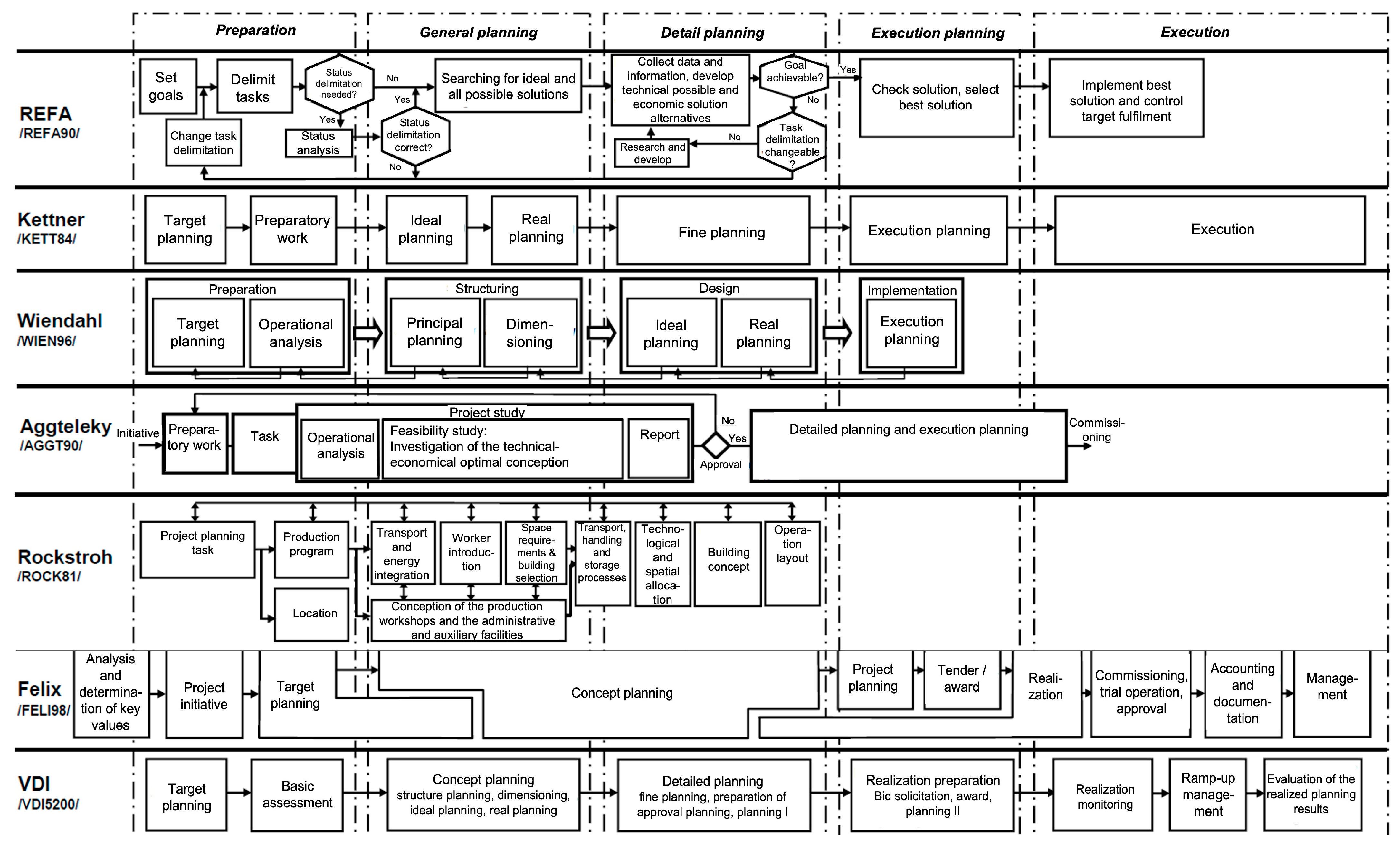
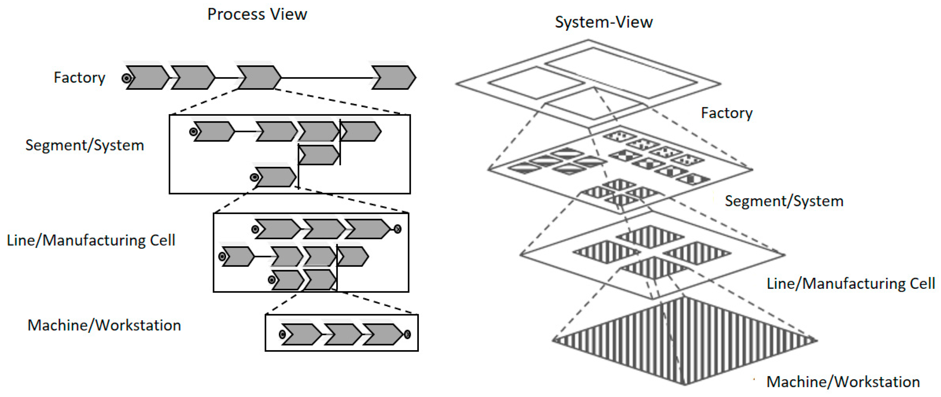
2.1. Relevant Research on Factory Planning

Factory planning is a structured multi-step process using various tools and methods for designing and dimensioning manufacturing systems [22,23,29,30,31,32,33,34]. The general planning process can be divided into several consecutive phases. Those phases address different aspects of the planning process at different stages and have individual levels of granularity [23,33,35,36]. Most guidelines’ planning process starts with defining the project and factory goals (Phase I), then determining and acquiring the necessary basic information and preliminary planning (Phase II). Phase III, then, is the development of the general factory concept, considering aspects like structures, layout planning, or the definition of an ideal solution. Phase IV continues with adapting the ideal solution to the real world by integrating existing restrictions and further developing detailed planning. Figure 1 shows the phases and their content across various planning guidelines by different authors [22,29,31,37,38,39].
Against the backdrop of this paper, phase II is the most important. Within phase II, the general-planning phase, factory planners must decide what kind of technology they want to apply and what products will be manufactured through what technology [22,31]. Most importantly, the planners also decide, at this stage, what kind and level of flexibility the production systems will have and what technologies will constitute this flexibility [18,40]. The decisions made at this point set the framework according to which the consecutive, more detailed planning steps must be aligned. Furthermore, the description, analysis, and quantification of processes, resources, and the general structure of the production system must be based on a system-theoretical foundation and guided by the principle of self-similarity [18,35,41,42,43]; i.e., by using the same elements and connection types within each iteration, planning results can be aggregated and divided across different planning stages and systematic layers within the production systems structure. This is exemplified in Figure 2.
This ability to describe processes and systems using the same elements across different levels of granularity is highly important. The reasons for this are threefold. Firstly, manufacturing products of almost any kind is a rather complex, multi-stage process. In order to organize and implement this process as efficiently and effectively as possible, most production systems and factories are designed in a specific way [22,23,34]. The fundamental idea at this point is to subdivide the factory based on either certain manufacturing processes or certain technologies used based on certain products and their characteristics [46,47,48,49].
An example of the first aspect is the manufacturing of a car. In this case, the press shop, the paint shop, and the assembly are three different sub-systems of a factory. They are, however, organizationally distinct within the overall structure. The assembly, for example, can then (in a higher level of granularity) be broken down into different sub-systems responsible for different parts and components (e.g., front end, engine, wiring harness, etc.). The same accounts for the process chain. Here, the overall process of the pressing of the body might be broken down into the different elements of the body itself: the door panels, side panels, frame side rail, or floor assembly. These processes can then be broken down into the necessary single forming processes.
In the case of the second aspect (the subdivision of factories following products and their characteristics), the example of medical syringes might be applicable. Medical syringes come in all different forms and shapes. From an efficiency point of view, it does not make sense to manufacture all different types on the same machines. Diameters, materials, length, width, and a lot of other parameters vary. Therefore, it makes sense, economic-wise and factory-planning-wise, to define various sub-systems within the factory, that each manufacture a different type, subset, or product variant. The decision on what variants and products to combine in a given segment can be made based on criteria like volume, sales predictability, and customer segments. For further information on this topic, please refer to [22,46,47,48] and the cited literature.
In order to integrate additive technologies into the overall flexibility design of manufacturing systems consistently, methods and tools quantifying this impact must meet these requirements. For the strategic integration of additive manufacturing technologies into the overall flexibility concept of a manufacturing system, it is, therefore, key that these principles of self-similarity and process orientation are met.

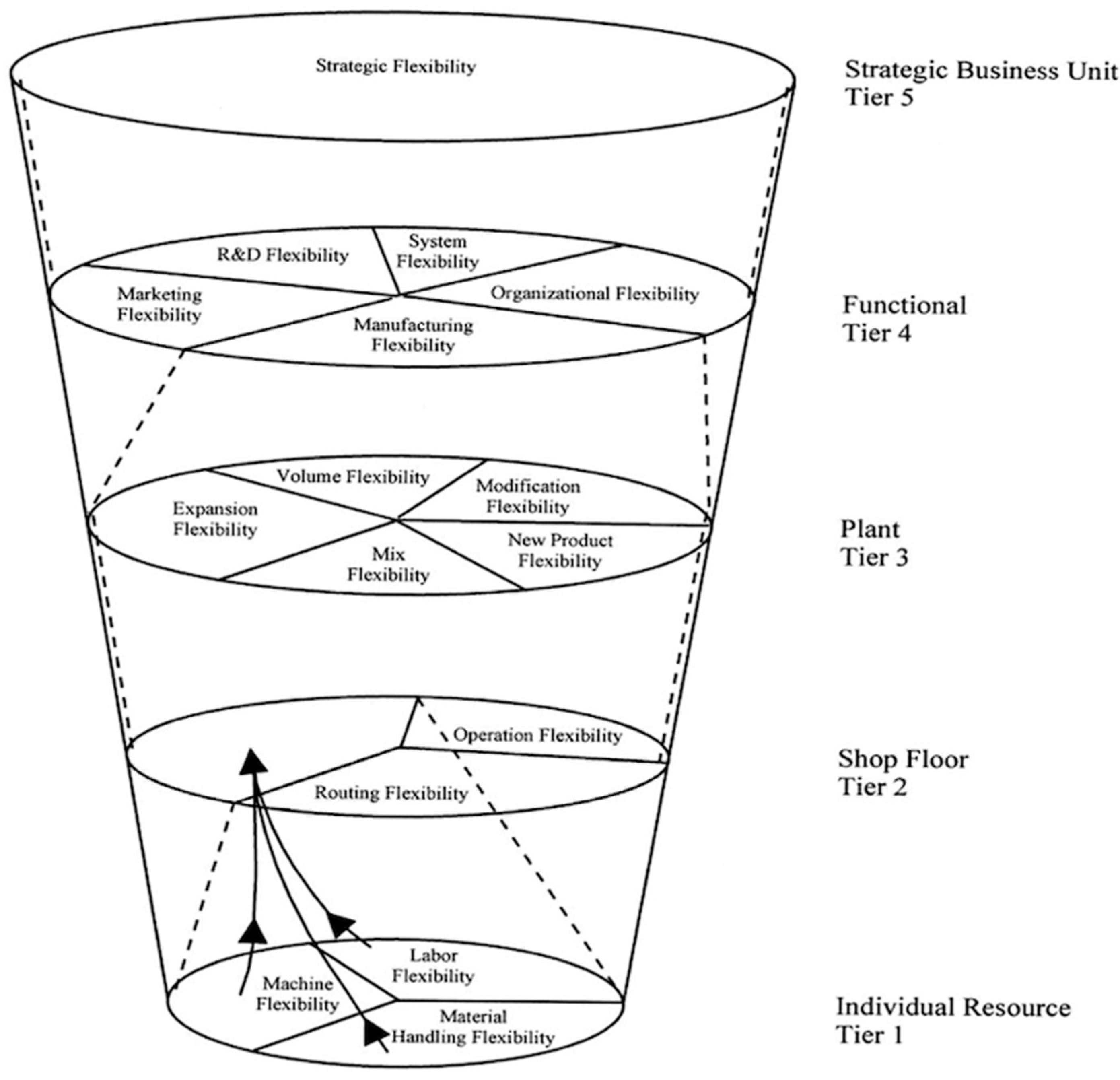
2.2. Relevant Research on Manufacturing Flexibility

The scientific research into the flexibility of production systems is nearly a century old, with the first works focusing on elasticity, the ability of a company to adjust to changing markets [50,51,52]. In the following decades, this relatively narrow view of elasticity was expanded continuously by including planning aspects, investment decisions, or the design of changeable organizational structures [53,54,55,56,57]. In the 1970s and 1980s, Jacob, Meffert, and others coined the term ‘flexibility’ and further expanded the concept [58,59,60,61]. Depending on the personal view of the respective authors, flexibility can be seen as the ability of a production system to actively counter changes in the environment, reorganize itself quickly, or operate efficiently in a given manufacturing corridor [62,63]. In the 1990s, Schewchuck and Moodie listed more than 70 definitions of manufacturing flexibility, and Sethi and Sethi identified upwards of 50 different types of flexibility [64,65]. To structure the different types of flexibility and establish a hierarchical order, Sethi and Sethi designed the first hierarchical framework for manufacturing flexibility [64]. This framework was picked up, expanded, and transferred to a prototypical organizational hierarchy by Koste and Malhorta [66], as shown in Figure 3.
By analyzing many publications related to flexibility, Koste and Malhorta carved out a hierarchical flexibility framework. This framework links different types of flexibility, locates them on different organizational levels within a production system, and shows what kind of flexibilities are constituted by what other lower types. The three dimensions of machine, labor, and handling flexibility are at the bottom of this hierarchy. These three core types or dimensions of flexibility constitute (at least to a significant degree) all other dimensions. Of those three, machine flexibility is recognized as the most important one, quantifying the number and heterogeneity of the machine [66]. Of the higher flexibility dimensions, volume and mix flexibility are generally considered the most important, as they constitute a company’s ability to swiftly react to fluctuations or changes within the production program [18,19,66,67]. This hierarchical classification of different types of flexibility and the structured identification of the dependencies between them is one of the milestones of flexibility research. By applying the hierarchical classification, it is possible to determine the contribution of different manufacturing and logistical resources to a specific type of higher flexibility. Conversely, suppose a company intends to enhance a certain type of flexibility within one specific area. In that case, it is possible to deduct what kind of resources with what properties are needed.
Beyond the notion of a flexibility hierarchy, the framework developed by Koste and Malhorta has the advantage of locating the different types of flexibility at specific levels within the factory. As indicated in Figure 3, different flexibility types can be attributed to different layers or organizational units within the factory structure. These layers are labeled tier 1 to tier 5 in Figure 3. These tiers can generally be connected to the different layers within the factory described in Section 2.1. This makes it possible to connect the different types of flexibility to different layers in the factory and, thus, to different levels of granularity in the process allocation. Since this works both ways, it is possible to directly connect certain stages in the factory-planning process with different types of flexibility. By using self-similar models to describe the different layers of the production system and the processes, it is possible to incorporate this in the design process of the manufacturing system.
These considerations are especially important when considering integrating additive manufacturing technologies into production systems. By applying the logic described above, it is possible to seamlessly integrate additive resources and technologies both in the process chains and into the overall structure of the production system. The potential of AM technologies is directly linked to the printers and their versatility as individual resources. This potential can be quantified via basic types of flexibility like machine flexibility and then extrapolated up the flexibility hierarchy. In connection with a self-similar and process-oriented description model for production systems, it should be possible to quantify the impact of additive technologies on different types of flexibility and production systems as a whole. However, to do so, it is necessary to develop a flexibility model that allows for the simultaneous quantification of conventional and additive process chains and manufacturing logic. Based on the works and frameworks of [64,66], numerous models have been developed for the quantification of different types of flexibility (e.g., [68,69,70,71,72,73,74,75]). Multiple models have been developed, especially for analyzing and evaluating the volume and mix flexibility. Different modeling approaches have been used depending on the authors’ angle on manufacturing and flexibility and the desired results. Alexopoulos et al., for example, used a logic based on dampening systems in mechanical engineering and focused on the time a production system needs to react to a change in market demand for certain products [70,71,76,77]. Peláez-Ibarrondo and Ruiz-Mercader, on the other hand, used a combination of a break-even approach and a bottleneck-based capacity analysis to determine the volume and mix flexibility of a production system [78]. Schuh et al. [69] present an approach based on an object-oriented system concept with different classes and an inheritance model. The model focuses on the simulation of different future scenarios, their probability, and the evaluation of different adaptation strategies for the production system. Wahab, Wu, and Lee developed a two-stage reference model for determining manufacturing flexibility. In the first stage, a data envelopment analysis considering setup and manufacturing times is used to establish the efficiency of different machines for previously defined operations. The second stage integrates internal and external factors. The volume and mix flexibility determination is then based on time, costs, and variety [79]. A more cost- and risk-based approach was designed by Lanza, Rühl, and Peters [80]. In an OEE-based comparison of different product-system scenarios varying production volumes and mixes are simulated. The results of these simulation runs are then interpreted based on the generated costs and existing bottlenecks. In the second step, the impact of varying production volumes on the production system is analyzed [80]. A volatility-based approach is offered by [73,81]. The likelihood of potential changes in the system’s environment is rated and then connected to specific flexibility dimensions. The result is an assessment of the potentially necessary adaptations of the production system to counter those environmental changes. The real options approach to assessing product-mix flexibility was used by Georgoulias et al. [82,83]. Different investment options were analyzed and rated depending on their contribution to the mix flexibility of a given production system and the expected discounted payout. Schuh et al. present a cross-factory approach, which considers flexibility at the network level and focuses, at its core, on the mobility of production volumes between different production sites [84]. On the other hand, Daniels developed an approach for the flexibilization of the operations scheduling within the factory structure based on the work plan flexibility [85].
Two of the most comprehensive approaches for the analysis and quantification of manufacturing flexibility were presented by Rogalski [19] and Luft [18]. Both offer a detailed and cost-centered approach based on the available resources within the production systems, shift models, and general resource availability. Both mathematical models enable a differentiated analysis of the volume, mix, and development flexibility of manufacturing systems while simultaneously offering a cost analysis regarding the production system configuration against the backdrop of various production programs. Rogalski uses the theoretical maximum capacity as the upper limit of a potential flexibility corridor and the break-even logic to determine the lower boundary. The mean square deviation of the individual product-constraint profit optima from the system-optimal production profit is used to calculate the system’s flexibility [19]. On the other hand, Luft uses a task-based approach to quantify the different types of flexibility while also including human resources in the calculation. This allows for the quantification not only of manufacturing processes but also of assembly systems [18].
Various publications also address the potential impact of additive technologies on the flexibility of manufacturing companies or manufacturing supply chains.
A flexibility evaluation approach that explicitly encompasses additive technologies in the context of the flexibility of supply chains is presented by Alogla et al. [86]. The authors show that certain aspects of additive technologies, like the freedom of geometry, the absence of tooling, or the ability for on-demand production, can enhance the flexibility of supply chains. The volume flexibility is measured by the production systems’ capability to satisfy customer needs within a given timespan, determined by the customer’s acceptance of waiting for the product in question. The mix flexibility was measured based on the changeover times between different product families. During various scenarios, the authors showed that these types of flexibility within supply chains could be positively impacted by AM technologies.
Another example quantifying the potential impact of additive resources on a manufacturing supply chain is presented by Baumers et al. [20]. By building on the probability approach for the measurement of volume, mix, and delivery flexibility within supply chains developed by Beamon [87], the authors were able to show in a respective case study not only the potentially positive impact of additive technologies on these types of flexibility within a supply chain, but also its limitations.
Other works like Eyers and Potter’s studied how AM could improve flexibility within a supply chain, especially by optimizing the dynamic allocation of labor [28]. These findings were then repeated and expanded into different types of flexibility across 12 case studies covering various industrial sectors, product volumes, and technologies [24]. Another case from the automotive industry was presented by Delic and Eyers [25], looking at supply chain flexibility and performance. Using a partial least square structural equation modeling approach, they showed that integrating additive technologies into automotive supply chains can enhance flexibility and performance. Similar results regarding supply chain mechanisms and outcomes regarding the implementation of additive technologies were reported by Verboeket and Krikke [26]. Similar results and conclusions can be found with Moho Yusuf et al. [27], who looked at the aerospace industry, or Chung et al. [88] in the context of smart factories and interchangeable processes.

2.3. Further Research on Additive Manufacturing

Additive manufacturing and the respective technologies have opened up a vast field of research activities, ranging from detailed aspects of different manufacturing processes and materials (e.g., [89,90,91,92,93,94,95]) and design for additive manufacturing (e.g., [96,97,98,99]) to hybrid manufacturing (e.g., [100,101,102]), Industry 4.0 (e.g., [103,104,105]), and sustainability (e.g., [98,106,107,108,109,110]).
Out of this spectrum, not all contributions are directly relevant to strategic factory planning. However, flexibility quantification models addressing additive manufacturing processes must be designed to allow the integration of such technological advances without forcing a redesign of the model. They also need to be integrated into the overall structure of the factory in a second step. This underlines, even more, the need for a consistent self-similar and process-centered modeling approach that also considers a system-theoretic view [18,28].
The two most relevant areas of research are, on the one hand, the publications addressing the impact of additive technologies on the design of the factory itself, and, on the other hand, the publications that enable the quantification of additive process times and, especially, cost, sometimes early in the planning process and ideally without any prerequisites for additive machines or software.
Stittgen [97] and Kopf [98] presented the most promising contributions out of the first category. Stittgen offers a larger perspective on the manufacturing system and considers production logistics. He also considers heterogeneous build jobs. These build jobs are then set in relation to typical (conventional) production key figures such as manufacturing times or delivery deviation within the overall framework by Nyhuis and Wiendahl on manufacturing and logistics [22,111,112,113]. The analysis and evaluations were conducted for the laser powder bed fusion (LPBF) process. On the other hand, Kopf presents a quantification method for creating cost-efficient factory structures for AM that considers the data situation in the early manufacturing and strategic-planning phases. The author provides a model for the cost-oriented planning of manufacturing sequences of additive technologies, also with a focus on LPBF. The focus is on the serial application of the technology in an industrial environment with the primary goal of forecasting the costs for the AM process compared to other planning alternatives.
In the second category, the research into manufacturing cost and times in the domain of additive technologies, current research mainly focuses on quantifying costs per unit (e.g., [20,114,115,116,117,118,119,120]). Some approaches are also taking into account particular logical distinctions with conventional manufacturing processes, such as referring to shopfloor key figures; e.g., Fera et al. consider an overall equipment efficiency (OEE) calculation and the printer performance and capacity for heterogenous build jobs. Therewith, they developed a cost model that integrated a more operational view [121]. Baumers et al. include process failure as going beyond current AM cost models [122]. A progressive development can be recognized by looking at the overall development of cost models in the context of additive manufacturing; i.e., they build on each other, and, successively, more perspectives or key figures are integrated (e.g., [123,124,125,126]). Various approaches add substantial value to calculating specific additive manufacturing costs and the factors that might influence the printing times and the printers’ performance across various materials and technologies. However, they do not remarkably contribute to an integrated production system perspective and the overall quantification of manufacturing flexibility since they exclusively focus on the performance of the additive resources and the factors that might influence it. Nevertheless, since times and costs are integral to the strategic technology-planning process, these models provide valuable data that can be integrated into the planning process. The model developed by Hartogh and Vietor offers a means to estimate cost and processing times, especially in a very early planning stage [127,128,129]. In their works, Hartogh and Vietor use the mathematical model of the Sierpinski carpets and a dimensionless complexity key figure to approximate a comparative body of reference that can then be used to calculate printing times and cost for additive series production. The respective abstraction process of a body or part is shown in the following Figure 4.
Even though only homogenous build chambers with one object type can be calculated, the model offers distinct advantages regarding quantifying costs and times for additive parts within the strategic planning process. Since, for the abstraction, no other information is needed than the component height, volume, and surface area, the prediction algorithm can be applied without further specific knowledge and special AM software to calculate the potential manufacturing times and printing cost in a sufficient granularity for the strategic planning process. Another significant advantage against this work’s backdrop is the algorithm’s genericity, i.e., different additive processes can be quantified. As with most comparable AM models, this model, as well, only considers the build process. Pre- and post-processes are not assessed. [128]
As can be inferred from the current research activities around AM, the focus up to now is, with very few exceptions, not on positioning AM in the context of the overall production system; i.e., AM is not yet examined closely in the environment of various production resources and more comprehensive causal relationships, such as capacity utilization or interdependent production key figures. Instead, the AM process’ monetary aspect (costs/profit) is the decisive target variable [131]. Supporting this line of argument, Korner et al. explicitly suggested in their paper, after a comprehensive literature analysis, the need for AM cost models to be integrated into the whole production system [132].
Nevertheless, the existing research and approaches provide valuable input for a more holistic model. Since process times and manufacturing costs are two cornerstones of most existing flexibility models, the respective data must also be available for additive resources, should they be integrated into mathematical models quantifying systemic flexibility.

3. Problem Definition and Solution Process

Our proposal aims to provide a model that enables companies to integrate additive technologies into the strategic factory-planning process and subsequently into (existing) production systems. The mathematical model for analyzing and calculating the impact of additive technologies has to consider the iterative nature of the factory-planning process and the shifting levels of planning detail [35,133]. For the flexibility evaluation model, this means that the basic logic in which the necessary processes are formulated must offer a degree of self-similarity that allows for flexible granularity regarding the planning progress. Furthermore, the model and its application procedure must take into account the substitutive nature of additive technologies. All models, methodologies, and concepts analyzed by the authors compare different resources at each process stage and iteratively distribute the process of the individual products onto the different resources. This process-for-process approach does work for conventional production systems and resources within acceptable limits. However, it fails to address the ability of additive resources to substitute entire conventional process chains. The same applies to integrating post-processes for AM components, which is necessary to modify certain features of previously printed parts, like the surfaces.
In order to achieve this, we first present a modified process-description model based on the logic of the works of [18,134,135,136]. This basic task logic possesses the required self-similarity. It thus allows for the necessary fluid level of granularity in the analytics, but it has also already been applied in the context of flexibility analysis ([18]) and factory planning ([35,133]). Based on this logic, a mathematical quantification model for volume and mix flexibility and a corresponding application guideline were developed. Both the model and guideline were applied in various case studies, one of which will be presented in this paper.

4. Proposed Flexibility Quantification Model

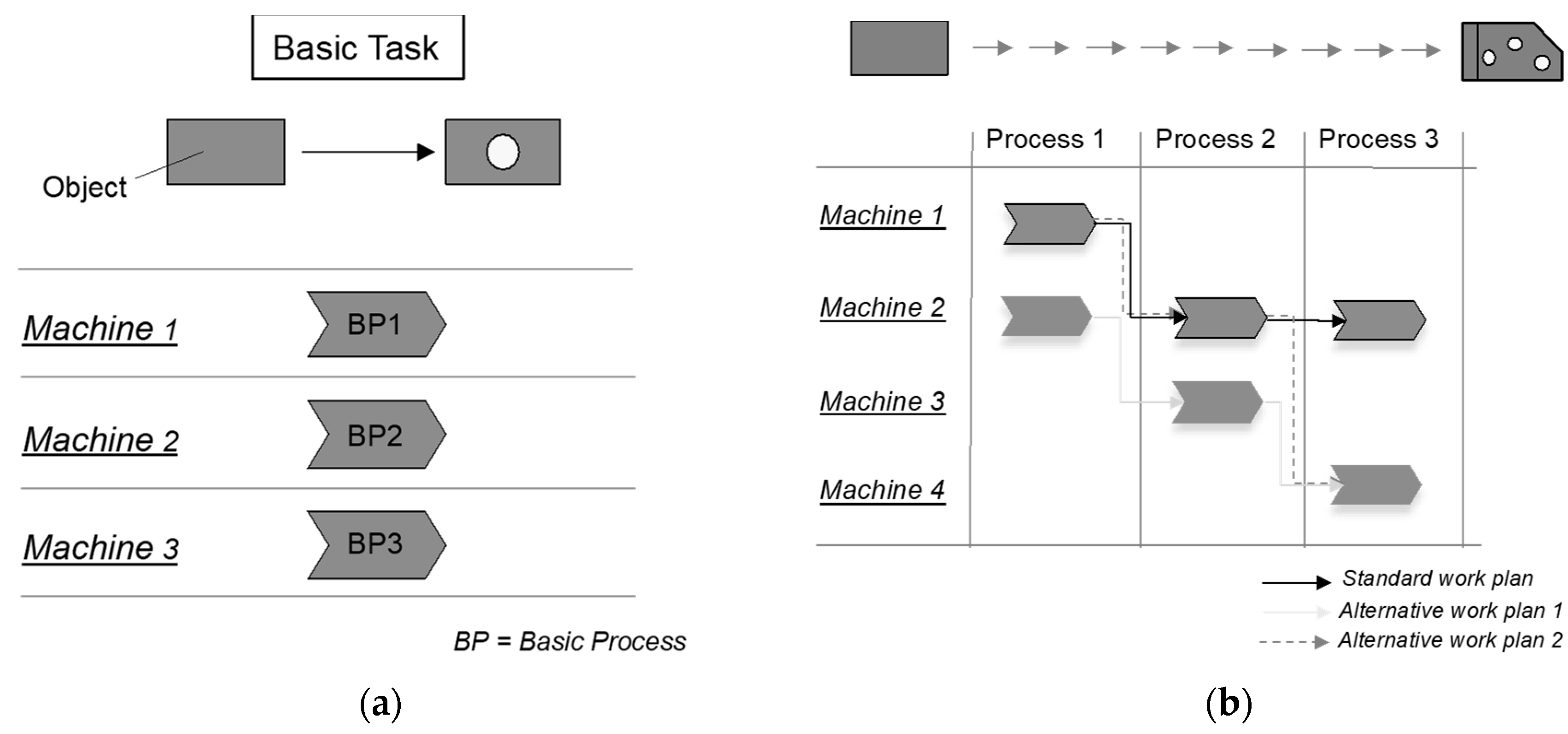
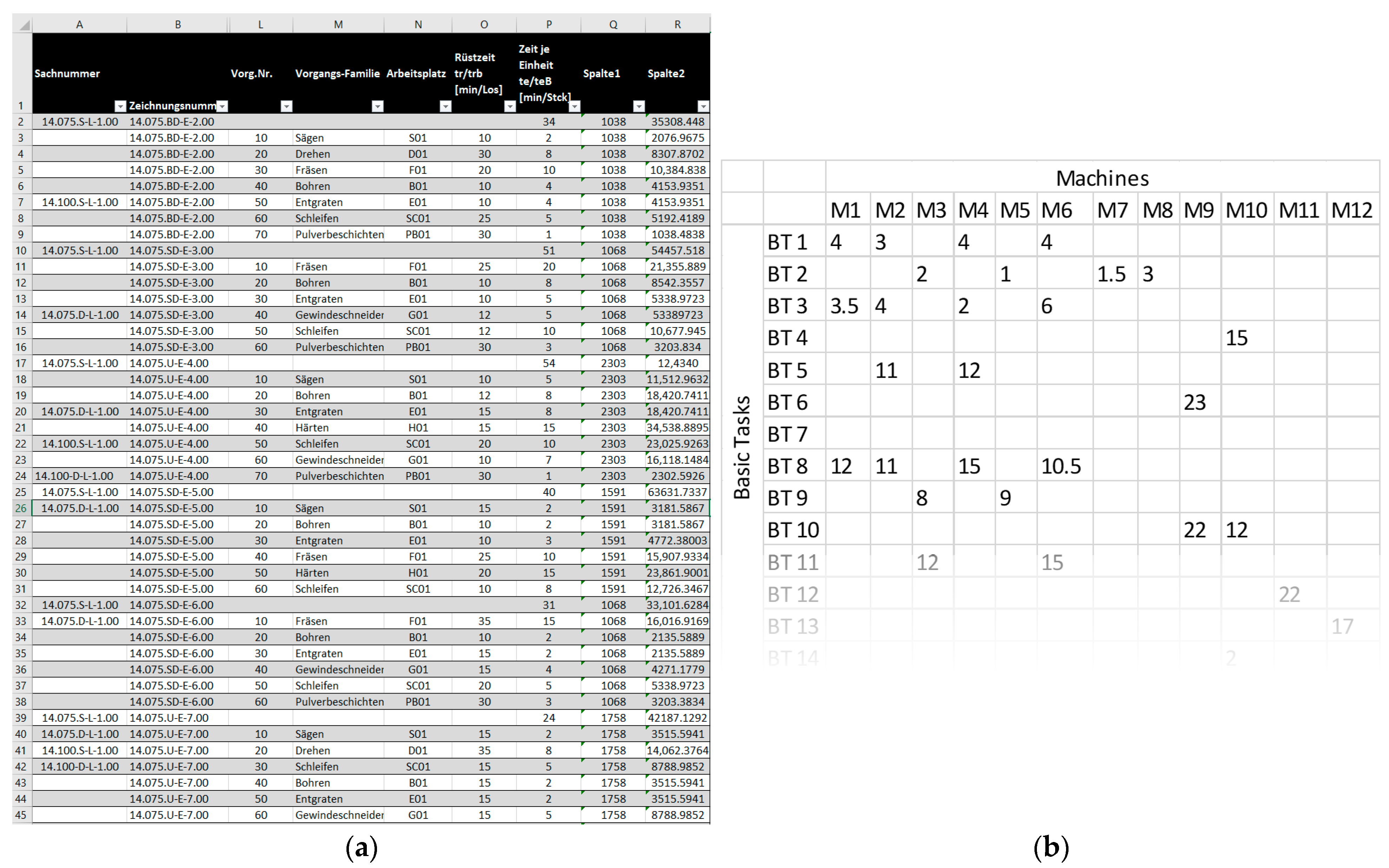
4.1. Basic Task Logic

For a quantification model to be of value in the early stages of the factory design and technology evaluation process, it must be based on a fundamental description logic. This, on the one hand, has to allow a continuous and fluid adjustment of the abstraction level (by means of self-similarity). On the other hand, the substitutional character of additive manufacturing technologies needs to be addressed. The conventional approach using reference work plans and tying processes at certain stages to specific machines’ respective technologies is not sufficient: there is a lack of flexibility in the alternating levels of detail as well as regarding the substitution potential of additive technologies.
For this reason, the authors chose a task-based approach [134,135] based on a process-centered logic for planning and designing production and logistical systems developed by Kuhn et al. [133,137,138,139]. This task-based approach was also applied by Luft [18] for the analysis, evaluation, and development of manufacturing flexibility in conventional production systems. Due to the fundamental process logic at the core of the model and the resulting self-similarity, there is a simple and frictionless adjustment of the level of granularity in the analysis and evaluation, as well as the integration of the substitution potential of additive technologies concerning conventional process chains.
The fundamental idea of the basic task logic is the separation or rather the separate answering of two questions, which, in manufacturing, are usually answered in one step. These questions concern the “how” and the “what” of each transformation within the creation process of a product within the manufacturing system [134,135,136]. These questions are generally answered by generating a work plan in which each necessary transformation (what) is directly linked to a specific machine (how). A core reason for the increasing complexity in manufacturing is created by directly answering these two questions in one stride. The direct link of transformation and means in one document (work plan) also means that every alternative regarding how the transformation can be achieved must also be described in a separate document. Furthermore, it severely limits the adaptability of models for flexibility analysis and evaluation since the same restrictions apply here [18].
In the context of strategic factory planning, this is especially challenging since with the definition of the work plans (even on a rather generic level), many technological questions are answered (and, thus, design options eliminated) at a stage where more flexibility and different design options would be highly beneficial [41,43].
In contrast to work plans, the task-based approach differentiates between tasks and processes. Tasks have both an external and an internal perspective. The external perspective encompasses respective goals (e.g., costs, performance, or efficiency) and objects (e.g., material and information). Against the backdrop of this paper, the primary goal would be the completion of a specific production program (with certain volumes and variants for a defined number of products) within a given time. The most relevant attributes of the objects would be the material (parts and components) necessary for the manufacturing of the production program across all intermediate levels, as well as the initial and final states of these objects related to each task.
Accordingly, the external view of tasks defines, through the exact specification of the respective initial and final states of the task objects along the respective task chain, two things: on the one hand, the logical sequence of the subtasks (pre- and post-events) and, on the other hand, the goals to which the activities for the fulfillment of a task are to be aligned. The activities whose correct execution results in fulfilling the corresponding task are described by the following set of characteristics, which represent the internal view of the task [18,134,136]. Namely, these are resources and methods. The resources are the productive performance potential (human and machine) within the respective production system. Methods, on the other hand, specify by which solution procedure (e.g., work steps), under which rules, and based on which basic principles the goals of a task may be reached. For this paper, the sequences of work steps and the corresponding work instructions, which determine the sequence of transformation tasks to be performed to produce a product (final task object) successfully, are of primary relevance. The process structures described by them determine the division of the production systems into organizational units and, thus, have a significant influence on the structure of a production system and, therefore, also on the levels of system flexibilities to be considered [18].
The execution of the activities necessary to fulfill the task is called a process [140] or an operation [136]. Compared to processes, tasks have more degrees of freedom in that the fulfillment of the task can be triggered by different prior events and, linked to this, also by different input objects, which means that alternative activities can fulfill the goal of a task [134].
The following Figure 5 graphically exemplifies the basic task logic and the concept of standard and alternative work plans.
The task pictured in Figure 5a is the creation of a hole inside the pictured object, the plate. The description of the necessary transformation at this stage would specify the whole, its diameter, tolerances, and so on. It would, however, not determine a specific manufacturing process. The connection of the task (creating the whole while adhering to all constraints) with a specific machine or manufacturing process will create the actual (basic) process. Depending on whether the whole will be created by using machine one, two, or three, it will create a different process. For the manufacturing process of a part or component, this means that there is one basic task chain describing all the necessary transformations. Each of these tasks can then be connected to one or more (different) machines capable of performing this task. A process chain or work plan is generated by combining different processes along the transformation process from raw material to finished part. Each work plan is just one manifestation of the initial basic task chain. This principle is exemplified in Figure 5b, with standard and alternative work plans as a standard means to allocate resources in modern production planning and the control of ERP (enterprise resource planning) systems.
The basic task logic was chosen as a theoretical foundation for the following flexibility model that considers conventional and additive production resources. It (the basic task logic) encompasses both self-similarity as well as a disjunctive description of the “how” and the “what” of a transformation in the context of manufacturing. Furthermore, the already-proven applicability of the basic task logic within the overall factory-planning process as well as the resulting simplification regarding the application of the developed model within this process advocated this decision. The same holds for the interpretation of the results.

4.2. Proposed Basic Mathematical Model

In order to provide potential applicants of the mathematical model with an as-easy-as-possible step-by-step approach, the description of the mathematical model is carried out in four steps. After reformulating the overall production program for conventional and additive manufacturing, the conventional part of the production system and the capacity restriction within will be addressed first. The same will then be performed for the part with additive resources. Since additive manufacturing often requires significant post-processing [1], which impacts the production system in terms of, for example, planning and resource availabilities, this will be added in step three. Subsequently, the formulation of an overall cost function follows, encompassing both types of resources and the post-processes.

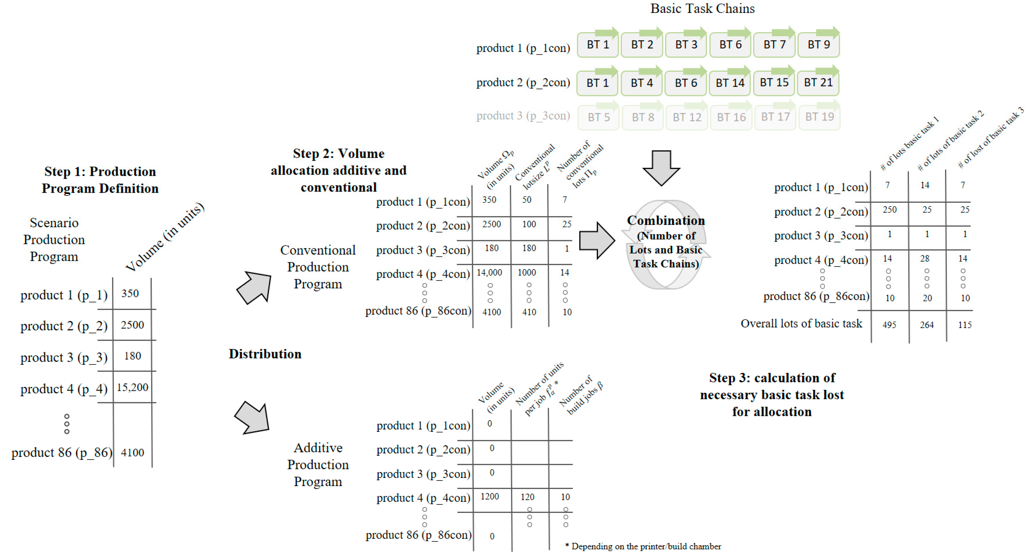
4.2.1. Reformulation of the Production Program

In order to calculate the capacity utilization additive and the conventional production resources (and, subsequently, the flexibility of the system) against the backdrop of a specific production program, it is necessary to reformulate this production program to fit the basic task logic. This reformulation is a three-step process. This process and the corresponding equation will be displayed first and then summarized in Figure 6. The definition of the respective overall production program in the respective scenario is step 1. The overall production program (PP) consists of a certain number of different products. Within every scenario analyzed, each product within the overall production program will be manufactured in a certain volume, in the following, labeled p_1 to p_o. On the level of the individual products, this can be described as follows:
PP ( p ) = p = ( p _ 1 , p _ 2 , p _ o )   with   p   ϵ   N ; o   ϵ   N
In order to make it compatible with the basic task logic and the mathematical model, the program must be divided into an additive and a conventional part. In the current developmental phase of the model, the factory planner has to decide on the precise distribution of the individual production volumes for each product. This is step two of the reformulation process. The assignment of a product to the conventional or the additive part does not have to be exclusive. Products can be manufactured additively and conventionally within one scenario. The planner has to determine what quantities of a product (e.g., p_5) will be manufactured additively (thus contributing to the additive part of the production program ( P P a d d p _ 5 ) and what quantities will be manufactured conventionally (thus contributing to the conventional part of the production program ( P P c o n p _ 5 ).
The following equation ensures that all production volumes for all products in the overall production program have been assigned to the additive or conventional production program:
P P ( p ) = P P a d d p + P P c o n ( p )
Since the mathematical model has to operate on different levels of granularity within the factory-planning cycle, it is necessary to make the description of the production program fit this requirement. Thus, the conventional and additive parts of the production program have to be formulated following the basic task logic. The conventional production program can be described as follows in the basic task logic:
B T i c o n = P P p c o n ° d i p c o n   w i t h   i = 1 , , n ; n   ϵ   0 N
In the equation above, d i p c o n represents the number of times a given basic task i has to be performed in order to manufacture or assemble product p. If, for example, the production p was a car and the task in question was the fitting of a tire; this task would have to be performed four times for each unit.
To make this model and the entire application procedure more applicable, especially for SMEs, the level of granularity chosen for the following discussions is the typical production lot since this is often used across various stages of the planning cycle. L p , thus, represents the standard manufacturing lot size for all basic tasks related to the product p. The demand for a product p ( Ω p ) within the conventional production program P P c o n ( p ) can thus be reformulated as Π p with manufacturing lots ( L p ) as follows:
Ω p L p = Π p   w i t h   a l l   p = 1 , , o   a n d   Π p   ϵ   N ; L p   ϵ   N , L p 0
Together with the calculation of the overall basic task demand (Equation (3)), this lot size calculation represents step 3 in reformulating the production program.
To ensure the consistency of the production program during the simulation runs, it is necessary to secure the manufactured production lots within each simulation run. This is achieved by comparing the number of necessary basic tasks B T i c o n with the number of allocated lots ( x i j p ) and the respective lot size ( L p ):
B T i c o n = p = 1 o j = 1 m x i j p L p   w i t h   i = 1 , , n
Following the reformulation of the conventional production program, the additive part must be adjusted as well. Since additive manufacturing does not take place in batches like conventional production, it is necessary to use a different metric to make the calculations compatible with the conventional and make them applicable within the factory-planning process.
For this purpose, the print job (J) has been selected as an appropriate level of granularity regarding the strategic capacity calculation. As was the case with the production lot in the dimension of conventional manufacturing, each print job contains a number of basic tasks. While it is theoretically possible to run this model with heterogeneous print jobs, only homogenous jobs are considered at this stage. Hence, only one type of basic task is contained in each job. Furthermore, each job must be defined specifically for an individual printer ( β ), containing a certain number of basic tasks of one specific type ( f α p ). This ensures that the number of basic tasks in the job will fit into the printer.
J β = f α p ; f N ; α 1 , , γ ; p 1 , , o | γ , o N w i t h   β = 1 , , δ ;   δ N
To ensure the completeness of the additive production program within each calculation, the number of basic tasks within all jobs printed must match the overall demand for all basic tasks:
B T α a d d = p = 1 o β = 1 δ y β f α p   w i t h   α = 1 , , γ ;   γ N
The following Figure 6 visualizes the three necessary steps in the reformulation of the production program and illustrates the overall procedure.
With the production program reformulated, the second step is the definition of the capacity restrictions both for additive and conventional resources.

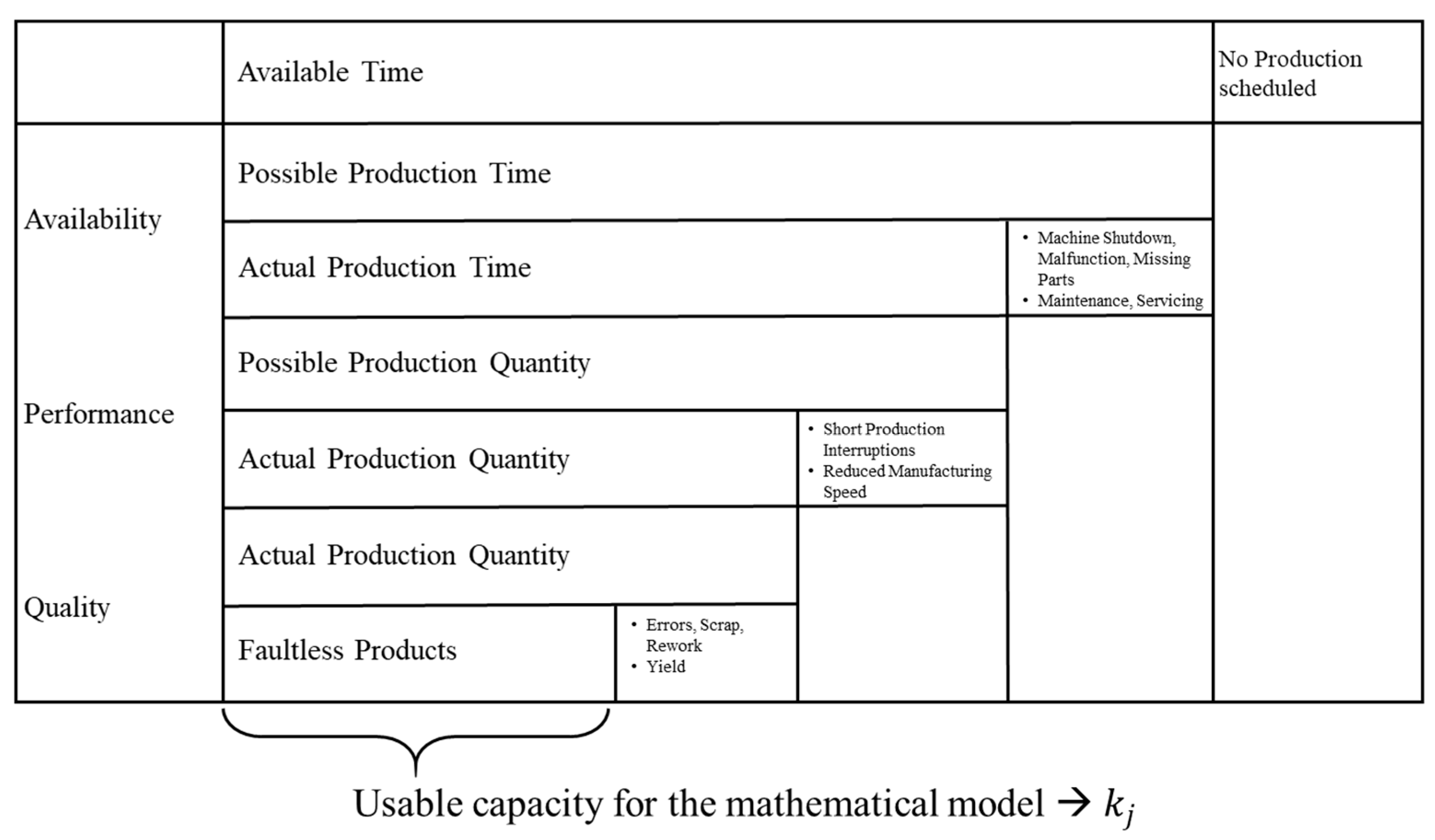
4.2.2. Capacity Restriction of Conventional and Additive Resources

To consider conventional and additive production resources, planners must first define the available capacity of these resources within the given period. The model focuses on the time component for both parts of the production system. At this stage, the authors presuppose that the geometrical capacity restrictions of the printers, as well as the technological feasibility for all resources and technologies, were evaluated beforehand. Regarding this model, all conventional resources j can be assigned a time-availability k j and all additive resources D a capacity time-availability k D . Both are referred to in the following as capacity.
The available capacity for a conventional machine can be defined in various ways. If no data are available, workforce members can offer an estimate based on their experience with the equipment. If the data in question are available in the existing IT infrastructure (e.g., the ERP system or MES), it can be used to specify the available capacity. However, to keep the estimate and, thus, the simulation results as realistic as possible, the authors suggest using the OEE, the overall equipment effectiveness. The OEE is a widely accepted key figure for measuring plant productivity [141]. As a key figure, the OEE identifies and classifies the unused potential of machines and industrial plants. It includes technical faults and losses that affect the performance of a production system. The general idea behind quantifying a system’s OEE is rather simple. It is a step-by-step procedure that considers several capacity-reducing factors. Based on a given production period (e.g., the duration of a to-be-analyzed scenario), the downtimes of the machine or plan are subtracted (step 1). In a second step, all occurring losses due to slowed operations are deducted. The third step is the deduction of the losses attributed to defective parts. This procedure leaves the planner with the period (capacity) available for manufacturing faultless products. Figure 7 shows the overall logic of the OOE and the different types of losses, together with examples.
The OEE approach for quantifying the available capacity within a given period is by no means mandatory. However, the authors strongly suggest using this approach as a structured means to establish the actual available capacity of a given production resource. For more information on the concept of the OEE as well as its differences, please consult the following literature [141,142]. The OEE logic can be applied to both conventional and additive production resources. Even though the fundamental manufacturing logic is different, the capacity-reducing factors addressed in the OEE logic still apply.
To ensure that the capacity of a conventional manufacturing machine is maintained, it is necessary to define the time a production resource j requires to process a lot of specific basic tasks assigned to a certain product p. For the factory-planning process, average setup and changeover times from product A to product B are sufficient. Scheduling considerations like in the research on flexible job-shop scheduling (e.g., [143,144,145,146,147,148,149]) are unnecessary. Thus, the time for processing a certain lot ( T i j p ) on a conventional machine can be formulated, taking into account the processing time of one basic task i on machine j ( t i j ), the lot size of product p ( L p ), and the average changeover time of machine j for basic task i ( t i j r ).
T i j p = L p t i j + t i j r
For conventional production resources, the capacity restriction, thus, can be formulated as follows.
i = 1 n p = 1 o x i j p T i j p k j   w i t h   j = 1 , , m
For the time restrictions on the additive resources, it is assumed that, for every build job defined for any given printer D, a corresponding time T β can be determined, which, in addition to the actual print time t β , also takes into account the time components for the preparation of the printer t β D ( u p ) and downstream times (e.g., removal of the parts) t β D ( d o w n ) of the printer. These are all times when the printer is occupied in any manner in order to fulfill the task and is not available for other operations. The time necessary to print a certain job T β on a printer D can, thus, be calculated analogously to the conventional production lots.
T β = t β + t β D ( u p ) + t β D ( d o w n )
The capacity of the printer over the considered time is, therefore, ensured by the number of jobs J β assigned to the printer D. The cumulative time to produce these jobs must be less than the available capacity of the printer k D , where y β represents the total number of jobs J β that were assigned to printer D during a simulation run using the quantification model.
β = 1 δ y β T β k D   w i t h   D = 1 , , E
For both the conventional and the additive resources, no negative lots might be assigned.
x i j p 0   a n d   x i j p N
y β 0   a n d   y β N

4.2.3. Integration of Post-Processing Processes

Due to the differences in the outcome of additive manufacturing processes compared to conventional ones (e.g., surface quality), it is often necessary to perform the so-called post-processing [5,150,151,152]. These are additional manufacturing steps that must be performed to, for example, remove support structures or enhance the surface of the product. These additional processes or steps must also be integrated into the model since they take up capacity that would otherwise be used solely for conventional manufacturing if performed on conventional equipment. In order to make the integration of those processes compatible with the overall logic, the calculation must also be lot-based. Generally, the factory planner can decide the lot size for the post-processing (as almost all external factors and aspects within this model) depending on the company’s situation. In this initial case, the lot size for the post-processing ( N B β ) will be equivalent to the number of basic tasks α, which are assigned to products p, within the previously defined jobs J β .
N B β = J β
The time required ( T β _ N B j ) for post-processing one lot of additively manufactured parts of a job β on a conventional machine j can be calculated analogously to the conventional batches. This is carried out using setup times t α _ N B j ( u p ) , processing time, and lot size.
T β _ N B j = N B β t α _ N B j + t α _ N B j ( u p )
For the conventional production resources, this results in the following adjusted capacity constraint, in which w β j describes the number of build jobs β to be post-processed on conventional machinery j.
i = 1 n p = 1 o x i j p T i j p + β = 1 δ w β j T β _ N B j k j   w i t h   j = 1 , , m
Again, the nonnegative constraint applies; i.e., no negative post-processing lots may be assigned, and these lots may always be processed completely and not split.
w β j 0   a n d   w β j ϵ N
The lot size of the post-processing must always be equivalent to the number of basic tasks within a given build job. This may be adjusted for scheduling reasons, logistics, or other operational requirements.

4.2.4. Overall Cost Function

The last relevant aspect of the mathematical model against the backdrop of factory planning is the integration of fixed and variable manufacturing costs. The general objective of the factory-planning process is the conceptual design of a manufacturing system that allows the manufacturing of the previously defined production program. Thus, the overall goal is the minimization of the cost, displayed in the following target function:
c t o t a l = j = 1 m p = 1 o i = 1 n x i j p c i j p + β = 1 δ j = 1 n w β j c β _ N B j + β = 1 δ y β c β + j = 1 m C j f i x + D = 1 E C D f i x
This function encompasses variable and fixed costs. The variable costs include the processing of conventional lots on conventional machines c i j p , the processing of post-processing lots on conventional machines c β _ N B j , and the variable costs of printing a job β ( c β ). The total variable costs incurred are also dependent on the number of actual lots ( z i p and w β j ) and jobs ( y β ) that get assigned to the various machines j and printers D. The fixed costs associated with the machines and printers within the production system are represented as C j f i x and C D f i x .

4.3. Necessary Input Data

Since the models’ intended use is as a tool for the strategic factory-planning process, it is necessary to define the different types. The two main aspects are the production system and the production program. For the successful application of the model, it is necessary that the initial production system definition, which poses the system-side framework for the analysis, contains the following details:
  • Number and type of machines;
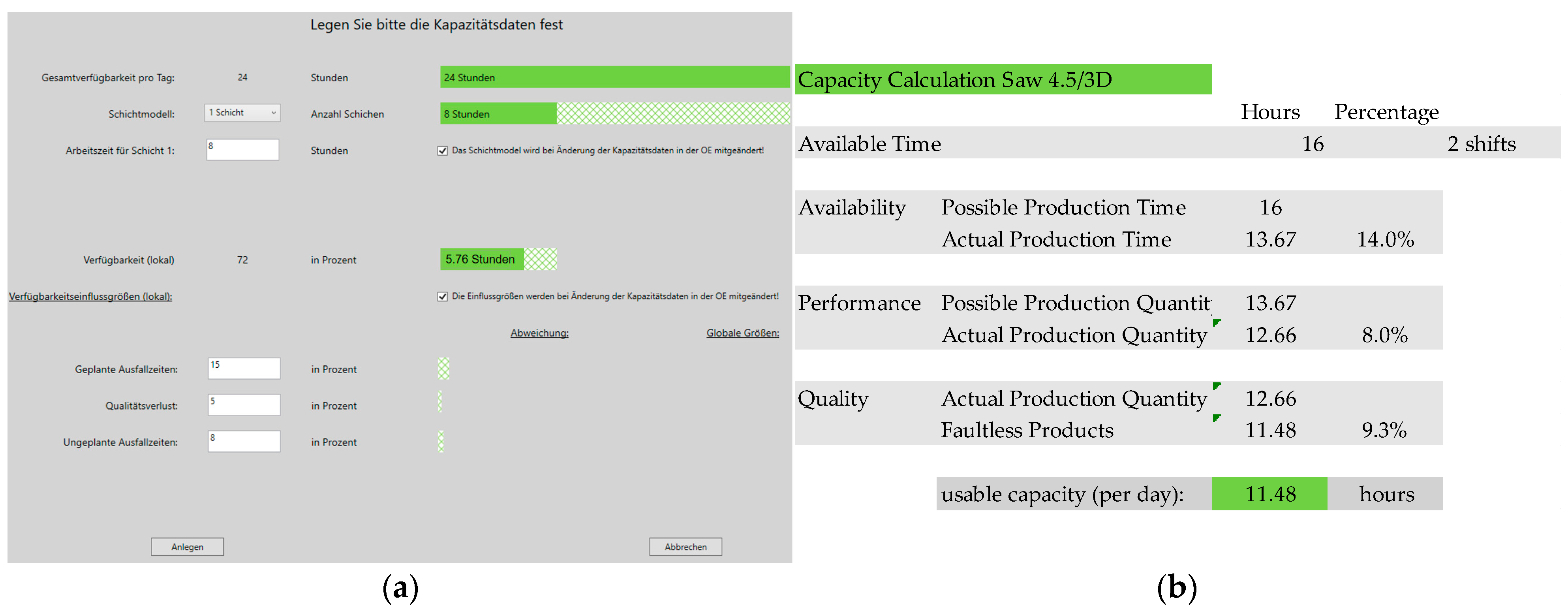
  • Available capacity for each machine;
  • Bill of materials (BoM);
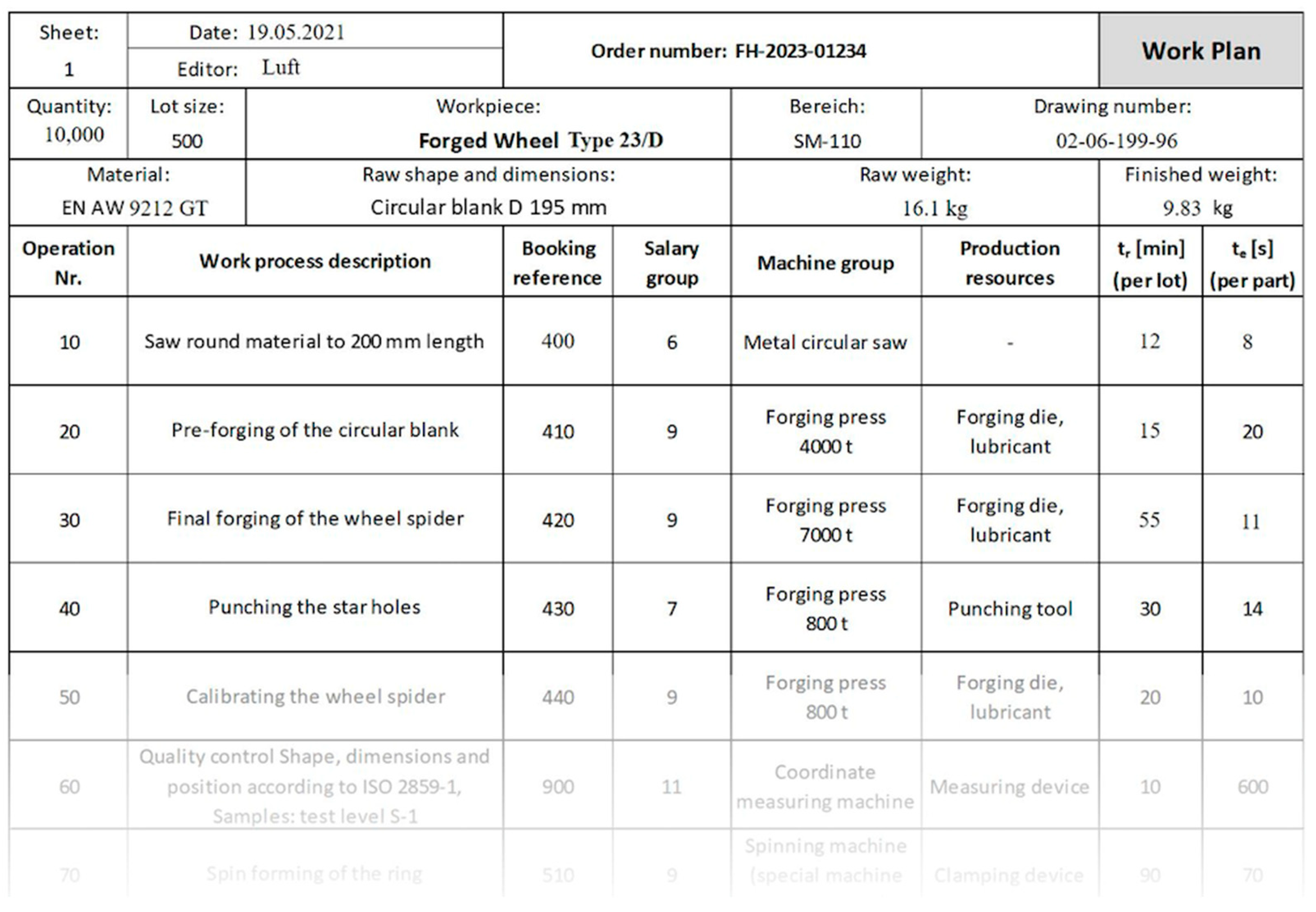
  • Work plans and alternative work plans for every product (including processing times);
  • Information/process plans for the conventional post-processing of additively manufactured parts;
  • Standard lot sizes for all products for the conventional manufacturing process;
  • Actual or calculated and quantified build jobs (printing times can be generated using the model developed by [127,128,129]);
  • Potentially available option for the flexibilization of the production system.
The definition of the production program, on the other hand, must contain the following information:
  • Number of different products;
  • Maximum anticipated production volume for every product;
  • Minimum anticipated production volume for every product;
  • Anticipated rate of substitution between all relevant products (relevant for the mix-analysis);
  • Timespan that is to be analyzed.
The options for the modification of the production program as well as the production system are consequently included in these initial framework conditions.

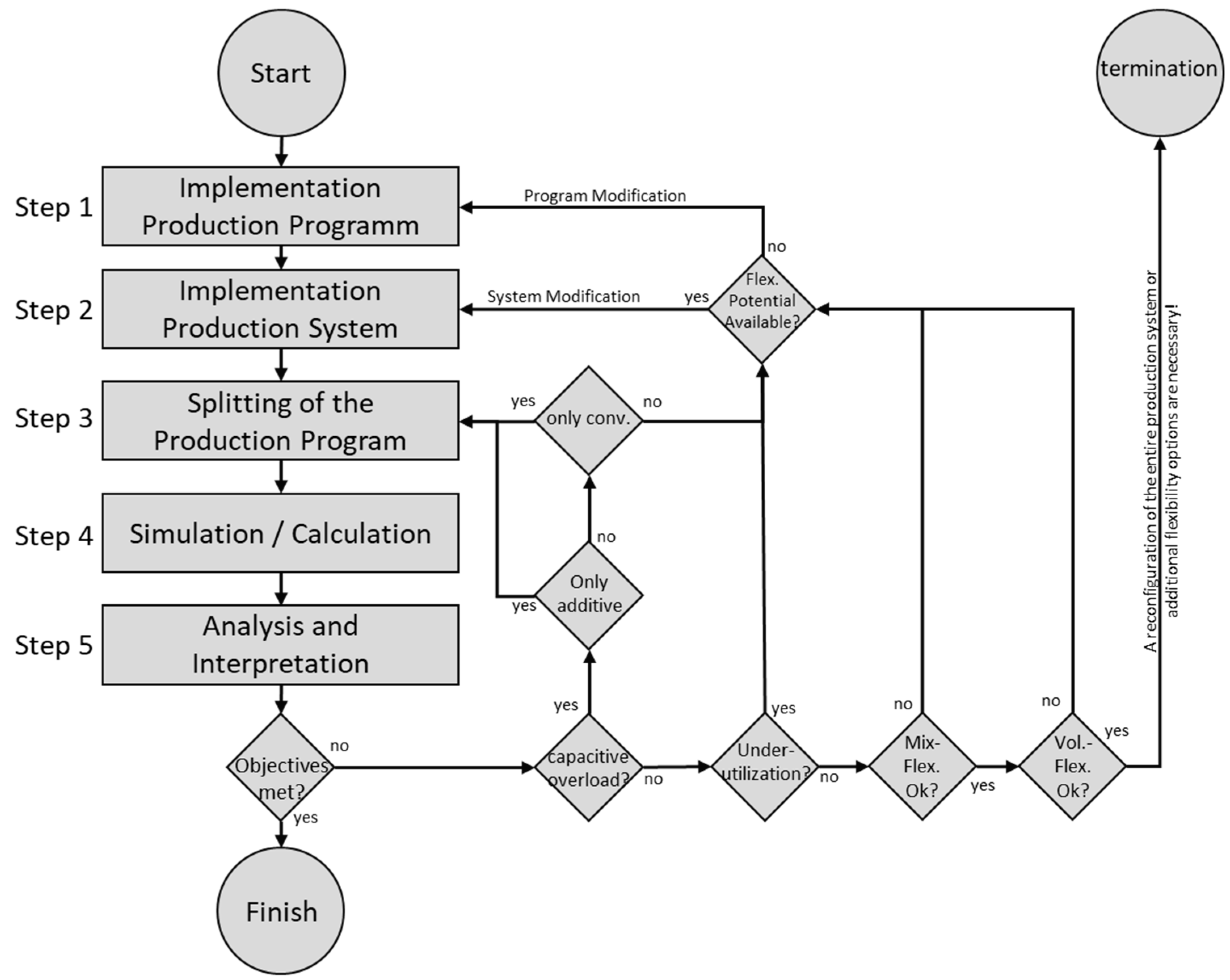
4.4. Proposed Methodology

From the perspective of a software system, a methodology represents a procedure or a step-by-step protocol designed to help with the application of the system [153]. Here, we propose a generic five-step guideline for people to apply the mathematical model. This guideline outlines the general steps needed to generate usable results for the factory-planning process. As a prerequisite, the overall target definition of the project and various pro-planning activities (such as generating the necessary input data) must have taken place already. A clear set of objectives compatible with the possible mathematical results must be in place. An example of a potential objective is the analysis of the volume and mix flexibility of a certain part of the production system against the backdrop of a set of previously defined production programs. Another example is the analysis and evaluation of new machines in the production system and their impact on aspects like cost and different types of flexibility. Moreover, the general structure of the production system, including its resources, must be defined. This means that all of the information described in Section 4.3 is available and has been checked for consistency. For the following steps and the exemplary flow chart displayed in Figure 8, it is assumed that compliance with the available capacity, satisfactory capacity utilization, and an acceptable cost structure, together with reasonable levels of volume and mix flexibility, are the main objectives.
Step 1 is the implementation of a starting version of the previously defined production program. The production program in question has to be defined beforehand as a part of the overall scenario. For every product in the production program, a certain range of potential production volumes was determined for a specific period of time. Since, usually, in the factory-planning process, a scenario analysis for the future production program is conducted, it is recommended at this stage to take the value with the highest entry probability as a starting point. The two central pieces of information for the production program are the timespan to be analyzed and the corresponding production volumes. An example of how the production program can be implemented is displayed in the case study in Section 4.5.2.
Step 2 is the implementation of the initial production system configuration. This includes all the information listed above, e.g., machines with their available capacity, work plans, bill of materials, or standard lot sizes for conventional manufacturing. As discussed in Section 4.2.2, it is advised that the logic behind the data determining the machine capacity is known and accepted by the model users. The suggested OEE logic was perceived as an acceptable common denominator by everybody within the participating company that provided the information for the following case studies. It is, however, not mandatory to use this metric. An example of how an implementation might look or be conducted is displayed in Section 4.5.2.
Step 3 then is splitting the production program into the part for conventional manufacturing and the part designated for the additive resources. There is no general rule on how to approach this at this stage. Planners should start with a rough estimate and then iterate to a more optimal solution. Suppose either the backup capacity of the model on the conventional side or the additive side is utilized within the simulation run. In that case, it is necessary to reallocate volumes to the other part of the production program. This logic is also displayed in Figure 8. The distribution and redistribution of volumes can be carried out in various ways within the software used for the calculations. In the implementation realized by the authors, different basic task chains were designed that could be directly connected with specific production volumes. Examples of this are displayed in Section 4.5.2.
Step 4 is the actual calculation itself. In order to achieve a minimum application hurdle, the model was formulated so that the calculations could be performed in Excel using a linear solver or comparable methods, depending on the complexity of the individual problem. Since the process of factory planning is in large part about the design of a flexible and robust production system, it is advised to take the initial production system configuration and test it against a broad range of production programs varying within the boundaries set by the planners initially. By generating these different scenarios, the necessary data for the latter interpretation of volume and mix flexibility can be generated.
The tools used for this calculation are up to the planner. These calculations can be performed using specific software for factory planning or can be conducted in Excel. Using factory-planning software might prove difficult, depending on the designed scenario. Most factory-planning solutions capable of this kind of machine-process allocation are based on the work plan logic. Thus, it might be difficult to implement the basic task logic. It is, however, also possible to implement the production program and the production system in Excel and then use a simplex algorithm or a different tool capable of optimizing these linear optimization problems. Examples of how this might look are given in Section 4.5.
Step 5, then, is the analysis and following interpretation of the generated results. Depending on the initially formulated results, this can be multi-dimensional. An analysis of the general capacity utilization and identification of potential bottlenecks are possible, as well as the quantification of the volume and mix flexibility of the production system against the backdrop of the previously defined and calculated scenarios.
Depending on the analysis results, there are various options for how the planner might proceed. If all the objectives have been met and none of the backup resources have been utilized, the scenario can be seen as concluded. The planner can then move on to a different scenario or start optimizing the structure of the production system based on the capacity utilization of the resources under consideration.
If the objectives have not been met, it is necessary to determine what kind of problem occurred. If the problem is a capacity overload in the conventional or additive part of the production system, the planner can try to redistribute volumes. In order to do so, it is necessary to analyze the capacity utilization of the considered production resources and then determine which resource has reached maximum capacity and what tasks have been assigned to the backup capacity. Based on this information, the planner can then redistribute limited volumes of the, for example, conventional production program towards the additive or vice versa.
If the capacity of the production system as a whole or of some machines specifically is not meeting the requirements defined beforehand, the planner can start to adjust the production system configuration. Depending on the analysis results, the planner can remove certain underutilized resources and restart the simulation. If the remaining capacity is sufficient, this will boost the overall capacity utilization and reduce the overall costs.
If the volume or the mix flexibility is insufficient, the planner has to choose between the adaptation of the production system (e.g., by adding new resources) or the modification of the production program. Since the production program often cannot be influenced by the company, adapting the system is usually the next step. The planner then has to determine what resources might be best to boost either type of flexibility. This, for example, can be achieved by comparing the individual capacity utilization of the machines within the system.
If none of the options described above is applicable, the planner has to terminate the analysis and the simulation, and fundamentally question the overall design of the scenario. Thus, either the production system configuration, the potentially addable resources, or the overall production program must be adjusted.
Figure 8 shows a simplified and compressed process for the model application to analyze a production system.
Depending on the results of the calculations and whether the objectives have been met, various iterations of parts or the entire process might be necessary to determine an acceptable production system configuration. The specific composition of the individual calculation runs can, of course, vary from time to time, depending on the project-specific requirements. The generalized process in Figure 8 shows a rather low level of granularity.

4.5. Case Study

4.5.1. Case Study Objectives

The objectives for the conduction of the case study were twofold. The first objective was the verification of the mathematical model in terms of the correctness of the calculated results. This was ensured by a double check of the calculated levels of capacity utilization against data generated by the company’s internal production planning as a scheduling system and separate calculations performed in a specific factory-planning software. Even though not all specifics could be modulated within those two systems, the results generated could be used to verify the mathematical model’s functionality and correctness regarding task allocation and capacity utilization.
The second objective was the analysis of a multitude of potential production systems’ configurations against the backdrop of an uncertain future, simulated by various production programs. During this process, the methodology of the scenario technique [40,154,155] was applied.
The target here was not to prove that manufacturing a part or component with additive technologies can be cheaper, even though that was the case in some scenario configurations. The overall objective was to evaluate whether the entire system would be more flexible when manufacturing fluctuating production programs. Thus, even if the additively manufactured part was more expansive than it would have been conventionally, the transition of this part to the additive resources enhanced the flexibility of the system for other parts and components disproportionately. Consequently, the additive resources contributed to the overall flexibility of the production system, even though the individual part on a printer, when looked upon in isolation, did not.

4.5.2. Background Information

A case study was generated with a co-operating company to verify the mathematical model. The company in question is in the process of expanding its product portfolio and is considering the increase in the production volume of various products. Due to various insecurities on the sales side, the company is already facing the challenge of varying production volumes of up to 200% for various products within its portfolio. Furthermore, the general capacity situation in the production system and the existing layout do not allow for the generation of isolated production sub-systems solely to manufacture a specific portion of the overall portfolio. Amidst these challenges, the company is considering using additive manufacturing technologies to compensate for demand fluctuations and enhance the production systems’ flexibility and unique selling proposition.
A sub-part of the existing production system containing processes like milling, hardening, turning, deburring, and laser-marking was isolated and used for the analysis. Furthermore, the company defined a corresponding production program with the required potential variations of the production volumes and potential shifts within the mix. In addition, the necessary post-processes were defined and quantified, and all the other necessary data (see Chapter 4.3) were generated.
During the analysis, various production system configurations and production programs were tested against one another. The general procedure followed the process described in this paper (Figure 8) and is described in extracts in the following chapters.
In order to simulate and analyze different scenarios, the company provided relevant information (e.g., the production layout, work plans, machines, shift models, maintenance intervals, costs, production volumes across different market scenarios, manufacturing lot sizes, potential interruptions, and scrap rates). Due to the existing confidentiality agreement, the original data cannot be published. The following Figure 9 shows an example of a standard work plan. The intention is to exemplify how the partnering company provided information. The work plan connects necessary transformations for manufacturing a product with machines. It also (among other things) specifies the processing and setup times and a basic process description of the transformation.
The information regarding the machines was provided in the form of an Excel file containing shift models, maintenance intervals, and other capacity-relevant information (please see Figure 7 for further relevant information).

4.5.3. Implementation of the Production Program

The production program was implemented, on the one hand, in Excel and, on the other hand, in a specialized factory-planning software that works on the basic task logic described earlier. The production program was implemented so that changes in volume and composition could be carried out with little effort. This was achieved by generating an initial consistency check that confirmed the conformity of the production program entered with the restrictions on lot sizes and build jobs described in Section 4.2.1. Different basic task chains were defined to facilitate the latter splitting of the production program. Therefore, specific parts of the production volumes could be directly connected with different work plans. For the additive part of the production program, this meant defining the basic tasks representing the print jobs and the necessary post-processes. The work plans were important for the conventional part of the production program (schematically displayed in Figure 10a). In a second step, the task–machine allocation specified in the different work plans has been abstracted and combined into a task–machine table, schematically displayed in Figure 10b. The table in Figure 10b also contains the individual machines’ processing times (in minutes).
The distribution of production volumes between the conventional and the additive part of the production system can be facilitated by changing the percentage of the overall volume between the different parts of the system.

4.5.4. Implementation of the Production System

The implementation of the production system was also carried out in Excel and the factory-planning software. The implementation included not only the data about machines, work plans, bill of materials, and the like, but also the implementation of certain flexibility options like backup machines or additional shifts, so that the potential development of the production system could also be considered up to a certain point.
Following the description of the capacity-relevant parameters in Section 4.2.2, different capacity-reducing aspects were considered and implemented. Figure 11a shows the implementation of these factors within the factory-planning software. The implementation within Excel followed the same logic. For consistency and acceptance reasons regarding the generated results, we recommend following the basic logic of the OEE description in Section 4.2.2. Figure 11b displays this for a machine that works in a two-shift operation.
The adherence to the OEE logic and its elements/components offers two distinct advantages. Firstly, the OEE is well-known in manufacturing companies, and its validity and elements are broadly accepted. Secondly, the differentiated breakdown of overall plant availability into individual factors enables a differentiated analysis of the potential of individual optimization points. In this way, conclusions can be drawn about where the production system should be optimized in the future.

4.5.5. Splitting of the Production Program

The production program was split by creating two versions of the new product. One version of the product was connected to various conventional work plans, and the other was connected to work plans containing additive processes and post-processing. In doing so, changes in the product allocation between additive and conventional could be made quickly. The allocation key was changed on a percentage basis to facilitate splitting without adjusting the overall production program.

4.5.6. Simulation/Calculation

The basic process for calculating capacity utilization, volume, mix flexibility, and the overall cost was based on comparing the scenario-specific production program with the scenario’s production system configuration. This was achieved based on different breakdowns of the overall production program into conventional and additive parts and alternations of the product mix within the production program.
The calculation of the different production programs and production system configuration was performed using a linear solver implemented in Excel as well as the factory-planning software. The calculations were performed for different production programs, production program allocations (conventional and additive), and production system configurations. The general target was, as stated before, to evaluate how an additively upgraded production system would change flexibility, capacity utilization, and costs.
The choice of the solver in Excel and within the factory-planning software was determined by the availability of the tools within the project and not based on performance considerations. The solver used for the calculations within Excel was What’sBest!, and that implemented in the factory-planning software was a simplex algorithm. The iterative process of changing the production program (within the parameters given by the partnering company), the production system modification, and the shifting of production volumes between the additive and the conventional part of the production system was repeated between 10 and 30 times until the calculated results offered no new insights into the scenario’s overall configuration. Then a new overall scenario for the factory plan was designed, and the process started again.

4.6. Results

4.6.1. Verification of the Mathematical Model

The application of the model within the described case study in conjunction with a specific factory-planning tool and the existing software for production planning within the partnering company allowed for a conclusive analysis and verification of the proposed mathematical model. The backup calculations performed in these systems showed that the basic-task–machine allocations generated using the mathematical model were consistent and did not violate any capacity restriction. The calculated costs were also within the acceptable margin of error for the designated task, namely, the rough assessment of the strategic production system design. Furthermore, the fuzziness regarding the setup times and other capacity-reducing aspects, which could not be modeled exactly due to the relatively high level of aggregation in the general-planning phase, remained within an acceptable range.

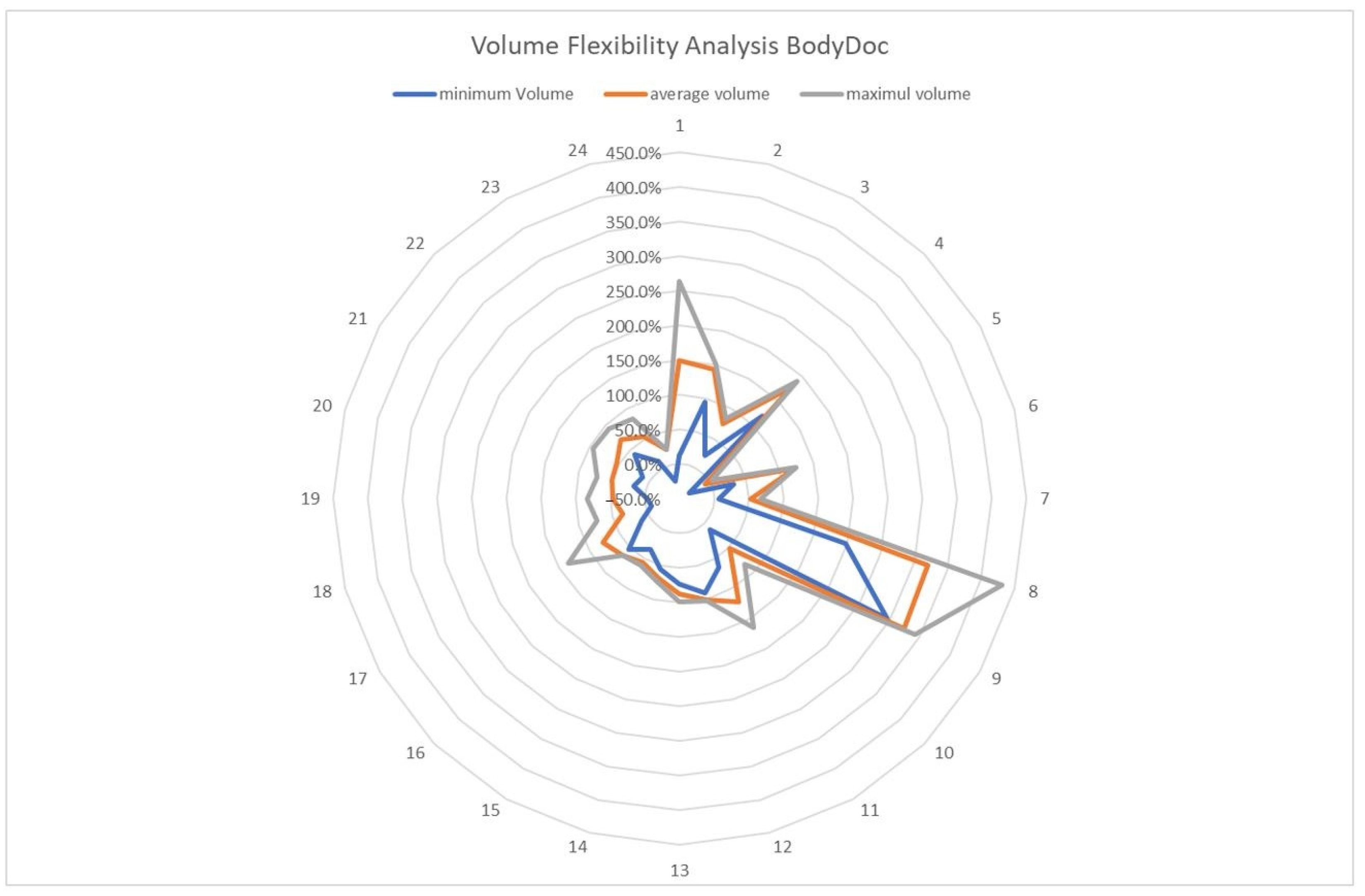
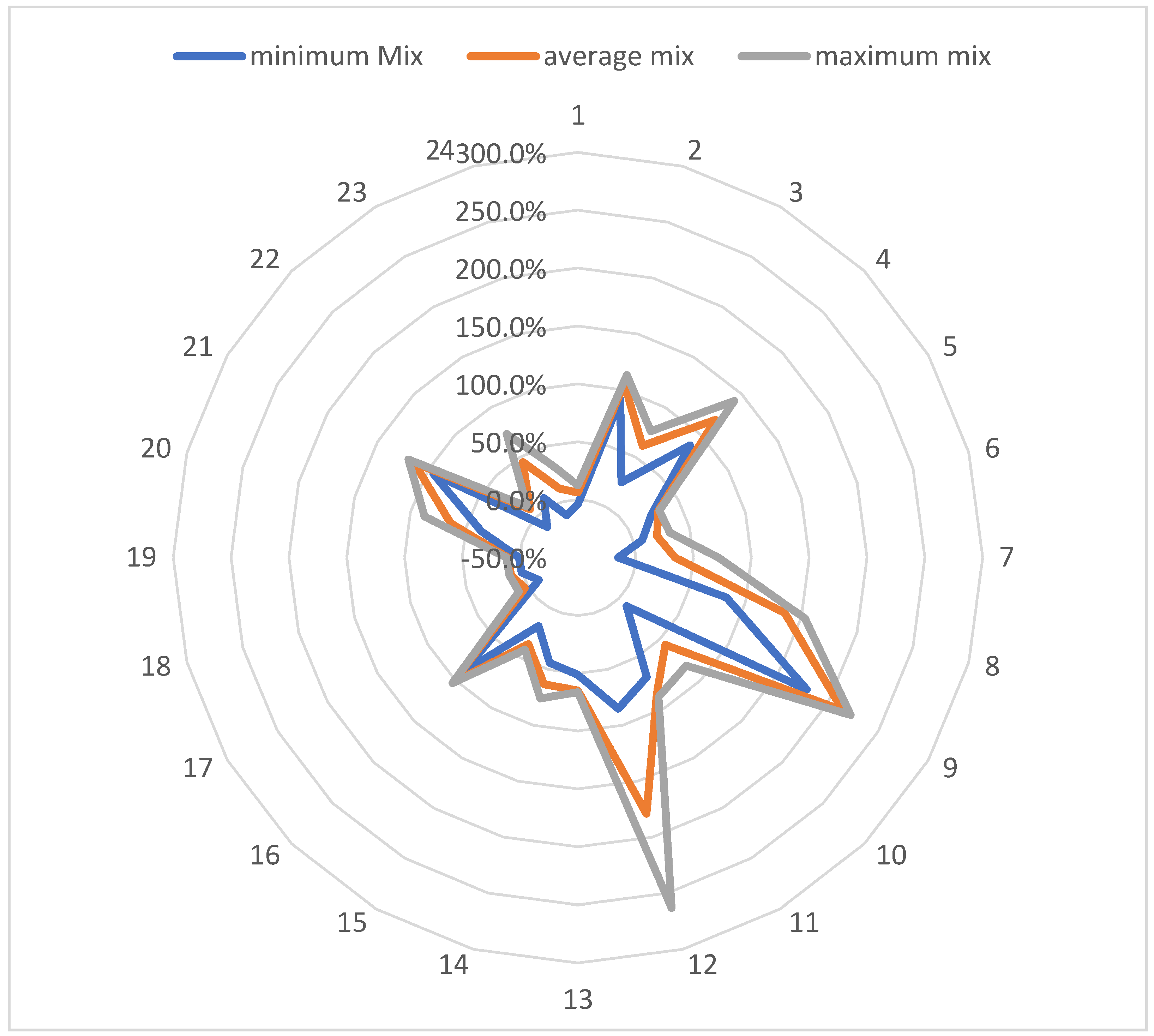
4.6.2. Cost, Volume, and Mix Flexibility

The calculated results of the different simulation runs were analyzed, interpreted, and, in the case of the flexibility assessment, used to set the benchmark of the production system again without additive resources. The following figures show different aspects of the analysis across various scenarios. The scenarios displayed within the figures always comprised a fixed production system configuration. This configuration was then tested against changing production programs or varying part allocations between the conventional and the additive part of the production program. Figure 12 shows the development of the calculated costs of a specific product across 20 different scenarios. The product in question was manufactured additively and conventionally across all scenarios. Figure 12 displays the maximum, minimum, and average cost for the product within each scenario across all production programs and program mixes tested within each scenario.
The flexibility of the production system regarding the manufacturing of various parts and components was also analyzed across various scenarios. The analysis of volume and mix flexibility was set up so that these two dimensions could be measured across all parts of the production program. The scenarios were designed so that the overall production program was kept stable, and only one part (in the case of the volume flexibility) or a pair (in the case of the mix flexibility) would be altered. The analysis did not focus on a specific part that was manufactured additively but rather on the impact of the additive manufacturing of a part on the entire production system and the overall production volumes.
The following two figures show a subset of volume and mix flexibility results. In Figure 13, the volume flexibility of the production system regarding the manufacturing of a specific item C is displayed across various scenarios.
The most interesting aspect of this analysis was that the biggest gains in volume flexibility (scenarios eight and nine) were achieved when shifting a different part (not part C) towards additive manufacturing, thus freeing manufacturing capacities within the conventional system and significantly boosting the output of part C. This effect can mostly be attributed to a bottleneck situation within the conventional part of the manufacturing system that was then eased up with the reallocation of one part towards the additive resources.
The analysis of the mix flexibility followed the same pattern, with the difference that two parts were chosen out of the production program. The production volume of one of these parts was then reduced to zero, with the rest of the production program kept the same. The question to be answered then, as an indicator for the production system’s mix flexibility, was how much the maximum producible production volume increase would be. The following Figure 9 shows the volume flexibility across various scenarios. This analysis was performed with various pairs of parts across different production system configurations and programs. Each scenario (1 to 24) in Figure 14 represents one part-pair within a number of production programs measured against a specific production system configuration and shows the changes in the level of volume flexibility that could be achieved. During the analysis of the mix flexibility, specific attention was paid to the question of how much the integration of additive resources and the subsequent reallocation of production volumes within the system impact the overall mix flexibility of the production system. This was, amongst other things, achieved by monitoring the capacity utilization of the additive resources compared to the conventional ones and the distribution of the overall production program among additive and conventional resources. All measurements were carried out against the backdrop of a purely conventional production reference system.
As seen in Figure 2 and Figure 3, the integration of additive resources can substantially affect production systems’ volume and mix flexibility. The effects are, however, not always positive or substantial enough to justify the integration of these new technologies. The calculations performed by applying the mathematical model showed that looking at a specific component and its manufacturing with additive technologies is a much too limited view of the question of how additive technologies can enhance production systems. Within various scenarios, the biggest impact was achieved by cost advantages not when looking at a single part or component, but rather when looking at the overall capacity utilization, the capacity bottlenecks within the production system, and the products using these scarce resources. Even though the current case study only looked at a small part of the production system and did not take into account the company’s entire production program, the analyses showed that the contribution AM can make to manufacturing must be viewed against the larger background of an entire production system and a more heterogeneous production program. Positive effects on volume and mix flexibility often occurred due to alternative task-capacity allocations that were only possible due to the additive manufacturing of a small part of the overall production program.

5. Discussion

The development of the mathematical model for the quantification of volume and mix flexibility for production systems containing additive technologies in the context of strategic production system design and planning offers new insights into what contribution these technologies may offer. The approach reduces a gap in the existing research for strategic factory planning when it comes to the quantification of the potential impact of additive technologies on the overall performance of the production system. More specifically, the model and the application offer an opportunity to quantify the contribution to the key success of factory volume and mix flexibility. Even though the calculations are made on the level of general capacity planning and scheduling issues that are not in scope yet, the results offer a good estimate of what additive technologies can achieve if integrated in a rather holistic way in the context of the entire production system. Due to the general setup of the model and the underlying structure of the basic task logic, CAD or STL files of products are not necessary. Calculations for AM build times can be performed based on the data generated by approximate methods like the model of Hartogh and Vietor, which lowers the initial investments (e.g., software and personal) and makes the model more applicable in the early planning stages, when additive technologies, the respective software, or the necessary skillset might not be available within the company on a sufficient level.
However, it should be noted that, even though both additive and conventional manufacturing processes can be calculated and evaluated within one manufacturing system and in the context of a single total cost function, the model does not allow for a single production program; i.e., it is necessary to split up the overall production program and then use an iterative approach to determine the best distribution of tasks between the additive and the conventional part of the production system. This step does increase the necessary planning effort and might prolong the identification of the best achievable solution.
Following this line of argument, the model and the application guideline in their current state only provide a tool for calculating solutions planners have designed in the first step and then the consecutive iterative optimization based on the interpretation of the results. The tool cannot determine the ideal configuration of the production system or what kind and type of machines should be integrated with which quantities. The same holds for further aspects like personal factors and skills, logistics, or the entire field of the structural restrictions of the buildings and the specific requirements additive technologies have on these dimensions. The mathematical model focuses only on production capacities, tasks, and processes. This, however, is sufficient for the strategic capacity planning within the overall factory-planning process and the technology planning within [22,23,33,34,35,36,42].
The proposed mathematical model was designed to quantify the two core types of flexibility, volume and mix flexibility. This was achieved, as demonstrated with the case study. However, as shown in Figure 3, these types of flexibility are only two out of many. In order to fully assess the flexibility of production systems comprising additive and conventional resources, it is thus necessary to assess the remaining types of flexibility and create a holistic and consistent model that allows for the quantifying of all aspects of the flexibility concept in the field of manufacturing, and, subsequently, the contribution additive technologies can make to it.
The case study used to verify the basic functionality and correctness of the mathematical model is not inclusive of all possible aspects, and some limitations should be noted. The main challenge for the application of the model is the necessary database. The required data contain numerous pieces of information that are most often unavailable in manufacturing companies. Chief among those is the alternative work plans and, thus, the necessary process times for the manufacturing lots in machines other than the standard work equipment. This information usually exists in the form of implicit knowledge in the heads of the employees but is not easily accessible for strategic capacity planning.
Following the line of argument regarding the availability of various pieces of information within the production system (e.g., alternative work plans), the basic task logic used to connect all this information into the overall factory-planning process is also not implemented widely. Nevertheless, describing the transformation performance to be achieved in a production system in a disjunct way regarding the available production resources and the respective technologies is an essential step. This not only holds true for factory planning but also targets the core of Industry 4.0 and the decentralized and service-oriented future of manufacturing in general [156,157,158,159,160,161,162,163].
The last point is that the mathematical model is designed to assist strategic planning. It consequently lacks applicability in the operational domain, where additional restrictions and requirements apply. Tasks like operational scheduling and production sequence planning are outside the scope of the current solution. However, the fundamental structure of the model is also applicable for this kind of tasks. The premise is that the process-chain-substituting ability of additive resources can be modeled in a way that does not disproportionately increase the number of machines and processes in the system.

6. Conclusions

In the literature on additive manufacturing technologies and manufacturing flexibility, the focus is often on comparing the conventional manufacturing process of a product versus the additive way. This is then analyzed and interpreted across the dimensions of cost, volume, and mix flexibility or lead times within a single company or across a supply chain [20,24,25,26,27,28]. No studies, however, examine the potential implications of additive technologies within a larger picture and, most notably, in an early phase of production or factory planning. The analysis of the impact of additive technologies on manufacturing in the context of an entire manufacturing (sub-)system in combination with a production program consisting of numerous different products with fluctuating demands has not been addressed so far. This is especially important because much of a production system’s flexibility is determined during early planning [18,19,22,23,42].
To gain further insights and to offer some degree of assistance within this planning phase, a mathematical model, together with a corresponding guideline, was developed. It builds on a task-based and process-oriented description logic for production and logistical systems and the modification of existing flexibility models. This novel model and the corresponding guideline allow for the analysis of volume and mix flexibility within production systems that contain both conventional and additive production resources. This allows for a scenario-based analysis and evaluation of various production system configurations against altering production programs within the factory-planning process. This approach enables planners to determine a system’s volume and mix flexibility and how manufacturing costs and capacity utilization of specific resource configurations fare against changing market demands. Thus, planners can design more flexible, robust, and adaptable factory solutions.
The developed model was tested against a modified application use case with a partnering company. During these tests, the model addressed various core aspects of the strategic factory-planning process related to flexibility design. The model was used to analyze different production system configurations and to quantify their inherent potential regarding volume and mix flexibility. The analysis covered production system configurations containing only conventional production resources and hybrid production system configurations containing additive and conventional production resources. The model was specifically used to identify limiting factors (resources) within the conventional production system and mitigate these bottlenecks by shifting parts of the production program onto additive resources. This identification of potential capacity bottlenecks within the conventional production system, together with the ability for the targeted reallocation of limited amounts of the production volume to additive resources, enabled a new view on the strategic potential additive technologies can have on the design of different types of manufacturing flexibility. The model’s capability to calculate conventional and additive production resources together enabled a differentiated understanding of additive potentials at an early planning stage. This, in turn, allowed planners during the project to analyze and evaluate production system configurations that would otherwise not even have been considered. Especially, the opportunity for a low-effort analysis of a larger number of different production programs against a set of conventional and hybrid production system configurations enabled the development of more efficient and more flexible production system configurations containing both additive and conventional resources. In doing so, the developed model can be used to integrate additive technologies into the early factory-planning process. This gives planners new possibilities for designing and configuring more flexible production systems without the limiting framework conditions of conventional manufacturing technologies. These insights cannot be achieved by applying conventional models for flexibility assessment due to their incompatibility with the different AM-process logic and their limited integrability in a process-oriented factory-planning process.
The analysis of various production system configurations against numerous altering production programs showed that additive technologies hold great potential for the flexibilization of production systems. Depending on the production system configuration and the composition of the corresponding production program, the flexibility gains using additive technologies for some part of the production program led to volume flexibility gains of up to 425%. In the case of the mix flexibility, these gains exceeded 200% in some scenarios. The main insight, however, was that these flexibility gains were often not for the additively manufactured product but rather due to capacitive reallocations due to the shifts within the production program from conventional to additive and the subsequent gains in free conventional production capacity. The gains in flexibility, however, frequently came with higher costs for the additively manufactured product. However, this mostly depended on the efficiency and complexity of the alternative, conventional manufacturing process, and is very situational.
The results offered in this paper are only a small first step in the direction of an integral, more holistic approach when it comes to analyzing and evaluating the potential impact additive technologies can have on manufacturing flexibility. The developed model provides a first solution for the analysis and evaluation of production systems containing both conventional and additive manufacturing technologies. Our current research has only looked at two types of flexibility out of many (see Figure 3). In order to create a comprehensive picture of the flexibility of a manufacturing system encompassing additive technologies, more flexibility types need to be integrated and connected. The impact of AM concerning lead times and manufacturing complexity is also an increasingly relevant topic that should be considered with flexibility and complexity in mind. The task-centered logic for modeling transformational processes within manufacturing systems offered within this paper might serve as a starting point. Finally, the authors suggest more research on the interdependencies of strategic production system planning and additive resources. AM is an important part of today’s modern production systems and thus needs to be considered in conceptualizing and planning them as an integrative aspect.

Author Contributions

Conceptualization, A.L. and N.L.; methodology, A.L.; validation, A.L., N.L. and S.B.; formal Analysis, A.L. and N.L.; investigation, A.L.; writing—original draft preparation, A.L.; writing—review & editing, A.L. and N.L.; visualization, A.L. and N.L.; supervision, S.B. All authors have read and agreed to the published version of the manuscript.

Funding

This research received no external funding.

Data Availability Statement

Not applicable.

Conflicts of Interest

The authors declare no conflict of interest.

References

  1. Associates, W. Wohlers Report 2022: 3D Printing and Additive Manufacturing Global State of the Industry; Wohlers Associates: Fort Collins, CO, USA, 2022; ISBN 978-0991333295. [Google Scholar]
  2. Parvanda, R.; Kala, P. Trends, opportunities, and challenges in the integration of the additive manufacturing with Industry 4.0. Prog. Addit. Manuf. 2022, 8, 587–614. [Google Scholar] [CrossRef]
  3. Tahmasebinia, F.; Jabbari, A.A.; Skrzypkowski, K. The Application of Finite Element Simulation and 3D Printing in Structural Design within Construction Industry 4.0. Appl. Sci. 2023, 13, 3929. [Google Scholar] [CrossRef]
  4. Abdullah, F.M.; Al-Ahmari, A.M.; Anwar, S. An Integrated Fuzzy DEMATEL and Fuzzy TOPSIS Method for Analyzing Smart Manufacturing Technologies. Processes 2023, 11, 906. [Google Scholar] [CrossRef]
  5. Gebhardt, A. Understanding Additive Manufacturing: Rapid Prototyping, Rapid Tooling, Rapid Manufacturing; Hanser Publishers: Munich, Germany; Cincinnati, OH, USA, 2012; ISBN 978-1-56990-507-4. [Google Scholar]
  6. Wacker, J.-D.; Kloska, T.; Linne, H.; Decker, J.; Janes, A.; Huxdorf, O.; Bose, S. Design and Experimental Analysis of an Adhesive Joint for a Hybrid Automotive Wheel. Processes 2023, 11, 819. [Google Scholar] [CrossRef]
  7. Kausar, A.; Ahmad, I.; Zhao, T.; Aldaghri, O.; Eisa, M.H. Polymer/Graphene Nanocomposites via 3D and 4D Printing—Design and Technical Potential. Processes 2023, 11, 868. [Google Scholar] [CrossRef]
  8. Attaran, M. The rise of 3-D printing: The advantages of additive manufacturing over traditional manufacturing. Bus. Horiz. 2017, 60, 677–688. [Google Scholar] [CrossRef]
  9. Nationale Akademie der Wissenschaften Leopoldina; Union der deutschen Akademien der Wissenschaften; Acatech—Deutsche Akademie der Technikwissenschaften. Additive Fertigung: Entwicklungen, Möglichkeiten und Herausforderungen: Stellungnahme; Deutsche Akademie der Naturforscher Leopoldina e.V.—Nationale Akademie der Wissenschaften; Union der deutschen Akademien der Wissenschaften e. V; acatech—Deutsche Akademie der Technikwissenschaften e. V: Halle (Saale)/Mainz/München, Germany, 2020; ISBN 978-3-8047-3636-8. [Google Scholar]
  10. Sing, S.L.; An, J.; Yeong, W.Y.; Wiria, F.E. Laser and electron-beam powder-bed additive manufacturing of metallic implants: A review on processes, materials and designs. J. Orthop. Res. 2016, 34, 369–385. [Google Scholar] [CrossRef] [PubMed]
  11. Harun, W.; Manam, N.S.; Kamariah, M.; Sharif, S.; Zulkifly, A.H.; Ahmad, I.; Miura, H. A review of powdered additive manufacturing techniques for Ti-6al-4v biomedical applications. Powder Technol. 2018, 331, 74–97. [Google Scholar] [CrossRef]
  12. Denkena, B.; Krödel, A.; Harmes, J.; Kempf, F.; Griemsmann, T.; Hoff, C.; Hermsdorf, J.; Kaierle, S. Additive manufacturing of metal-bonded grinding tools. Int. J. Adv. Manuf. Technol. 2020, 107, 2387–2395. [Google Scholar] [CrossRef] [Green Version]
  13. Zhang, L.-C.; Liu, Y.; Li, S.; Hao, Y. Additive Manufacturing of Titanium Alloys by Electron Beam Melting: A Review. Adv. Eng. Mater. 2018, 20, 1700842. [Google Scholar] [CrossRef]
  14. Revilla-León, M.; Sadeghpour, M.; Özcan, M. A Review of the Applications of Additive Manufacturing Technologies Used to Fabricate Metals in Implant Dentistry. J. Prosthodont. 2020, 29, 579–593. [Google Scholar] [CrossRef]
  15. Khorasani, M.; Gibson, I.; Ghasemi, A.H.; Hadavi, E.; Rolfe, B. Laser subtractive and laser powder bed fusion of metals: Review of process and production features. Rapid Prototyp. J. 2023, 29, 935–958. [Google Scholar] [CrossRef]
  16. Ravalji, J.M.; Raval, S.J. Review of quality issues and mitigation strategies for metal powder bed fusion. Rapid Prototyp. J. 2023, 29, 792–817. [Google Scholar] [CrossRef]
  17. Kunkel, M.H.; Gebhardt, A.; Mpofu, K.; Kallweit, S. Quality assurance in metal powder bed fusion via deep-learning-based image classification. Rapid Prototyp. J. 2019, 26, 259–266. [Google Scholar] [CrossRef]
  18. Luft, N. Aufgabenbasierte Flexibilitätsbewertung von Produktionssystemen; Verl. Praxiswissen: Dortmund, Germany, 2013; ISBN 978-3-86975-084-2. [Google Scholar]
  19. Rogalski, S. Entwicklung einer Methodik zur Flexibilitätsbewertung von Produktionssystemen; Universitätsverlag Karlsruhe: Karlsruhe, Germany, 2009; ISBN 978-3-86644-383-9. [Google Scholar]
  20. Alogla, A.A.; Baumers, M.; Tuck, C.; Elmadih, W. The Impact of Additive Manufacturing on the Flexibility of a Manufacturing Supply Chain. Appl. Sci. 2021, 11, 3707. [Google Scholar] [CrossRef]
  21. Koste, L.L.; Malhorta, M.K.; Sharma, S. Measuring dimensions of manufacturing flexibility. J. Oper. Manag. 2004, 22, 171–196. [Google Scholar] [CrossRef]
  22. Wiendahl, H.P.; Reichardt, J.; Nyhuis, P. Handbuch Fabrikplanung: Konzept, Gestaltung und Umsetzung Wandlungsfähiger Produktionsstätten; Hanser: München, Germany, 2009; ISBN 978-3-446-22477-3. [Google Scholar]
  23. Burggräf, P.; Schuh, G.; Dannapfel, M.; Swist, M.; Esfahani, M.E. Fabrikplanung, 2., Vollständig Neu Bearbeitete und Erweiterte Auflage; Springer Vieweg: Berlin/Heidelberg, Germany, 2021; ISBN 978-3-662-61968-1. [Google Scholar]
  24. Eyers, D.R.; Potter, A.T.; Gosling, J.; Naim, M.M. The flexibility of industrial additive manufacturing systems. Int. J. Oper. Prod. Manag. 2018, 38, 2313–2343. [Google Scholar] [CrossRef] [Green Version]
  25. Delic, M.; Eyers, D.R. The effect of additive manufacturing adoption on supply chain flexibility and performance: An empirical analysis from the automotive industry. Int. J. Prod. Econ. 2020, 228, 107689. [Google Scholar] [CrossRef]
  26. Verboeket, V.; Krikke, H. Additive Manufacturing: A Game Changer in Supply Chain Design. Logistics 2019, 3, 13. [Google Scholar] [CrossRef] [Green Version]
  27. Mohd Yusuf, S.; Cutler, S.; Gao, N. Review: The Impact of Metal Additive Manufacturing on the Aerospace Industry. Metals 2019, 9, 1286. [Google Scholar] [CrossRef] [Green Version]
  28. Eyers, D.R.; Potter, A.T. Industrial Additive Manufacturing: A manufacturing systems perspective. Comput. Ind. 2017, 92–93, 208–218. [Google Scholar] [CrossRef]
  29. Aggteleky, B. Fabrikplanung: Werksentwicklung und Betriebsrationalisierung, 2., Vollständig überarbeitete und Erweiterte Auflage; Carl Hanser Verlag: München, Germany; Wien, Austria, 1990; ISBN 3-446-15800-6. [Google Scholar]
  30. Wandlungsfähige Produktionssysteme. Heute Die Industrie von Morgen Gestalten; Nyhuis, P., Reinhart, G., Abele, E., Eds.; PZH Produktionstechnisches Zentrum GmbH: Garbsen, Germany, 2008. [Google Scholar]
  31. Richtlinie, V.D.I. 5200: Fabrikplanung. In Planungsvorgehen; Verein Deutscher Ingenieure: Düsseldorf, Germany, 2009. [Google Scholar]
  32. Grundig, C. Fabrikplanung. Planungssystematik—Methoden—Anwendungen, 3. Auflage; Hanser Verlag: München, Germany, 2009; ISBN 9783446442153. [Google Scholar]
  33. Pawellek, G. Ganzheitliche Fabrikplanung; Springer: Berlin/Heidelberg, Germany, 2014; ISBN 978-3-662-43727-8. [Google Scholar]
  34. Schenk, M.; Wirth, S. Fabrikplanung und Fabrikbetrieb. Methoden für die Wandlungsfähige und Vernetzte Fabrik; Springer: Berlin/Heidelberg, Germany, 2004; ISBN 978-3642054587. [Google Scholar]
  35. Beller, M. Entwicklung Eines Prozessorientieren Vorgehens zur Fabrikplanung // Entwicklung Eines Prozessorientierten Vorgehensmodells zur Fabrikplanung; Verl. Praxiswissen: Dortmund, Germany, 2010; ISBN 978-3-86975-026-2. [Google Scholar]
  36. Nöcker, J.C. Zustandsbasierte Fabrikplanung, 1. Auflage; Apprimus-Verl.: Aachen, Germany, 2012; ISBN 978-3-86359-059-8. [Google Scholar]
  37. REFA. Methodenlehre der Betriebsorganisation, Planung und Gestaltung Komplexer Produktionssysteme, 2. Auflage; Hanser: München, Germany, 1990; ISBN 3446159673. [Google Scholar]
  38. Kettner, H.; Schmidt, J.; Greim, H.-R. Leitfaden der Systematischen Fabrikplanung: Mit zahlreichen Checklisten; Hanser: München, Germany, 2010; ISBN 9783446138254. [Google Scholar]
  39. Rockstroh, W. Beitrag zur Projektierung Integrierter Fertigung im Zusammenhang mit der Entwicklung Automatisierter Betriebe; WissZ der TU Dresden: Dresden, Germany, 1981. [Google Scholar]
  40. Hernández Morales, R. Systematik der Wandlungsfähigkeit in der Fabrikplanung; VDI-Verlag: Düsseldorf, Germany, 2003; ISBN 3193149168. [Google Scholar]
  41. Kuhn, A.; Klingebiel, K.; Schmidt, A.; Luft, N. Modellgestützes Planen und kollaboratives Experimentieren für robuste Distributionssysteme. In Wissensarbeit—Zwischen Strengen Prozessen und Kreativem Spielraum; Spath, D., Ed.; GITO-Verlag: Berlin, Germany, 2011; pp. 177–198. ISBN 978-3-942183-51-2. [Google Scholar]
  42. Luft, N.; Wötzel, A.; Kessler, S.; Wagenitz, A.; Schmidt, A. Planung wandlungsfähiger Produktons- und Logistiksysteme. Ind. Manag. 2011, 27, 73–76. [Google Scholar]
  43. Kuhn, A.; Kessler, S.; Luft, N. Prozessorientierte Planung wandlungsfähiger Produktions- und Logistiksysteme mit wiederverwendbaren Planungsfällen. In Wandlungsfähige Produktionssysteme; Nyhuis, P., Ed.; GITO-Verlag: Berlin, Germany, 2010; pp. 211–235. [Google Scholar]
  44. Neuhausen, J. Methodik zur Gestaltung Modularer Produktionssysteme für Unternehmen der Serienproduktion; Dissertation, RWTH Aachen: Aachen, Germany, 2001. [Google Scholar]
  45. Ropohl, G. Allgemeine Technologie: Eine Systemtheorie der Technik: Eine Systemtheorie der Technik, 2nd ed.; Hanser: München, Germany, 1999; ISBN 3-446-19606-4. [Google Scholar]
  46. Wildemann, H. Die Modulare Fabrik, 5. Auflage; TCW, Transfer-Centrum: München, Germany, 1998. [Google Scholar]
  47. Wiendahl, H.-P.; Nofem, D.; Klußmann, J.H.; Breitenbach, F. Planung Modularer Fabriken; Hanser: München, Germany, 2005. [Google Scholar]
  48. Feser, B. Fertigungssegmentierung: Strategiekonforme Organisationsgestaltung in Produktion und Logistik; Deutscher Universitäts-Verlag: Wiesbaden, Germany, 1999; ISBN 978-3-8244-0459-9. [Google Scholar]
  49. Lopitzsch, J.R. Segmentierte Adaptive Fertigungssteuerung; IFA Hannover, Universität Hannover: Hannover, Germany, 2005. [Google Scholar]
  50. Schmalenbach, E. Die Betriebswirtschaftslehre an der Schwelle der neuen Wirtschaftsverfassung. Z. Handel. Forsch. 1928, 22, 241–251. [Google Scholar]
  51. Schmidt, F. Die Anpassung der Betriebe an die Wirtschaftslage. Z. Betr. 1926, 3, 85–106. [Google Scholar]
  52. Kalveram, W. Elastizität und Betriebsführung. Z. Betr. 1931, 8, 705–711. [Google Scholar]
  53. Öhlinger, W. Betriebselastizität, Die Anpassung des Industriebetriebs an Sich Verändernde Wirtschaftsverhältnisse; Eigenverlag Publisher: Wien, Austria, 1935. [Google Scholar]
  54. Tannenbaum, R.; Massiarik, F. Leadership: A frame of reference. Manag. Sci. 1957, 4, 1–20. [Google Scholar] [CrossRef]
  55. Riebel, P. Die Elastizität des Betirebs; Westdt. Verlag: Köln, Germany, 1954. [Google Scholar]
  56. Preisnig, K. Das Elastizitätsproblem in der Werksorganisation; Inaugural Dissertation publisher: Nürnberg, Germany, 1957. [Google Scholar]
  57. Vormbaum, H. Wechsel zwischen den fixen Kosten und dem betriebswirtschaftlichen Elastizitätsstreben. Z. Betr. 1959, 29, 193–205. [Google Scholar]
  58. Meffert, H. Die Flexibilität in Betriebswirtschaftlichen Entscheidungen; Unveröffentlichte Habilitation: München, Germany, 1968. [Google Scholar]
  59. Meffert, H. Zum Problem der betriebswirtschaftlichen Flexibilität. Z. Betr. 1969, 39, 779–800. [Google Scholar]
  60. Meffert, H. Größere Flexibilität als Unternehmenskonzept. Z. Betr. Forsch. 1985, 38, 121–137. [Google Scholar]
  61. Jacob, H. Flexibilitätsüberlegungen in der Investitionsrechnung. Z. Betr. 1967, 37, 1–34. [Google Scholar]
  62. Eversheim, W.; Schaefer, F.-W. Flexibilität in der Produktion—Eine Voraussetzung zur Sicherung der Wettbewerbsfähigkeit von Unternehmen. In Handwörterbuch der Produktionswirtschaft; Kern, W., Ed.; Poeschel: Stuttgart, Germany, 1979; Volume 121, pp. 463–470. [Google Scholar]
  63. Schmigalla, H. Flexibel Automatisierte Fertigungssysteme; Gabler: Wiesbaden, Germany, 1994. [Google Scholar]
  64. Sethi, A.; Sethi, S. Flexibility in manufacturing: A Survey. Int. J. Flex. Manuf. Syst. 1990, 2, 289–328. [Google Scholar] [CrossRef]
  65. Shewchuck, J.P.; Moodie, C.L. Definition and Classifikation of Manufacturing FlexibilityTypes and Measures. Int. J. Flex. Manuf. Syst. 1998, 10, 325–349. [Google Scholar] [CrossRef]
  66. Koste, L.L.; Malhorta, M.K. A theoretical Framework for Analyzing the Dimensions of Manufacturing Flexibility. J. Oper. Manag. 1999, 18, 75–94. [Google Scholar] [CrossRef]
  67. Tempelmeier, H.; Kuhn, H. Flexible Fertigungssysteme: Entscheidungsunterstützung für Konfiguration und Betrieb; Springer: Berlin/Heidelberg, Germany, 1992; ISBN 3-540-55154-9. [Google Scholar]
  68. Ali, S.; Seifoddini, H. Simulation intelligence and modeling for manufacturing uncertainties. In Proceedings of the 2006 Winter Simulation Conference, Monterey, CA, USA, 3–6 December 2006; pp. 1920–1928. [Google Scholar]
  69. Schuh, G.; Gulden, A.; Wemhöner, N.; Kampker, A. Bewertung der Flexibilität von Produktionssystemen: Kennzahlen zur Bewertung der Stückzahl-, Varianten- und Produktänderungsflexibilität auf Linienebene. Wt Werkstattstech. Online 2004, 94, 299–304. [Google Scholar] [CrossRef]
  70. Alexopoulos, K.; Papakostas, N.; Mourtzis, D.; Gogos, P.; Chryssolouris, G. Quantifying the flexibility of a manufacturing system by applying he ttransfer function. Int. J. Comput. Integr. Manuf. 2006, 20, 538–547. [Google Scholar] [CrossRef] [Green Version]
  71. Chryssolouris, G.; Georgoulias, K.; Papakostas, N.; Makris, S. A Toolbox Approach for Flexibility Measurements in Diverse Environments. In CIRP Annals—Manufacturing Technology; Issue I; CIRP: Singapore, 2007; Volume 56, pp. 423–426. [Google Scholar]
  72. Georgoulias, K.; Papakostas, N.; Mourtzis, D.; Chryssolouris, G. Flexibility evaluation: A toolbox approach. Int. J. Comput. Integr. Manuf. 2009, 22, 428–442. [Google Scholar] [CrossRef] [Green Version]
  73. Korves, B.; Krebs, P. Bewertung und Planung von Fabriken unter Flexibilitätsgesichtspunkten bei der Siemens AG. In Münchener Kolloquium-Innovationen für Die Produktion; Zäh, M., Hoffmann, H., Reinhart, G., Eds.; Herbert Utz Verlag: München, Germany, 2008; pp. 57–68. [Google Scholar]
  74. Zäh, M.F.; Müller, E.; von Bredow, M. Methoden zur Bwertung von Flexibilität in der Produktion. Ind. Manag. 2006, 22, 29–32. [Google Scholar]
  75. Zäh, M.F.; Müller, N. On planning and evaluating capacity flexibilities in uncertain markets. In Proceedings of the 2nd International Conference on Changeable, Reconfigurable, Agile and Virtual Production (CARV 2007), Toronto, ON, Canada, 22 July 2007. [Google Scholar]
  76. Alexopoulos, K.; Mourtzis, D.; Papakostas, N.; Chryssolouris, G. DESYMA—Assessing flexibility for the lifecycle of manufacturing systems. Int. J. Prod. Res. 2007, 47, 1683–1694. [Google Scholar] [CrossRef]
  77. Alexopoulos, K.; Mamassioulas, A.; Mourtzis, D.; Chryssolouris, G. Volume and product flexibility: A case study for a refrigerators producing facility. In Proceedings of the 10th IEEE International Conference on Emerging Technologies and Factory Automation: ETFA, Catania, Italy, 19–22 September 2005; Lo Bello, L., Sauter, T., Eds.; IEEE: Piscataway, NJ, USA, 2005. ISBN 0-7803-9402-X. [Google Scholar]
  78. Peláez-Ibarrondo, J.J.; Ruiz-Mercader, J. Measuring operational flexibility. In Proceedings of the Fourth SMESME International Conference, Stimulating Manufacturing Excellence in Small & Medium Enterprises, Aalborg, Denmark, 14–16 May 2001; pp. 292–302. [Google Scholar]
  79. Wahab, M.I.M.; Wu, D.; Lee, C.-G. A generic approach to measuring the machine flexibility of manufacturing systems. Eur. J. Oper. Res. 2008, 186, 137–149. [Google Scholar] [CrossRef]
  80. Lanza, G.; Rühl, J.; Peters, S. Bewertung von Stückzahl- und Variantenflexibilität in der Produktion. Z. Wirtsch. Fabr. 2009, 104, 1039–1044. [Google Scholar] [CrossRef]
  81. Zäh, M.F.; Müller, N. A Model for Capacity Evaluation under Market Uncertainties. Prod. Eng. Res. Dev. 2006, XIII, 201–210. [Google Scholar]
  82. Bengtsson, J. Manufacturing flexibility and real options: A review. Int. J. Prod. Econ. 2001, 74, 213–224. [Google Scholar] [CrossRef]
  83. Bengtsson, J.; Ohlager, J. Valuation of product-mix flexibility using real options. Int. J. Prod. Econ. 2002, 78, 13–28. [Google Scholar] [CrossRef]
  84. Schuh, G.; Gützlaff, A.; Thomas, K.; Ays, J.; Brinkmann, H. Flexibilitätssteigerungen im Produktionsnetzwerk. Z. Wirtsch. Fabr. 2020, 115, 581–584. [Google Scholar] [CrossRef]
  85. Müller, D. Flexibilitätsorientierte Selbststeuerung: Eine Methode für die Dezentral-Myopische Reihenfolgebildung in frei Verketteten Montagesystemen unter Verwendung von Arbeitsplanflexibilität, [1. Auflage]; Verlag Praxiswissen: Dortmund, Germany, 2020; ISBN 978-3-86975-154-2. [Google Scholar]
  86. Alogla, A.; Baumers, M.; Tuck, C. The impact of adopting additive manufacturing on the performance of a responsive supply chain. In Supply Chain Networks vs Platforms: Innovations, Challenges and Opportunities, Proceedings of the 24th International Symposium on Logistics (ISL 2019), Würzburg, Germany, 14–17 July 2019; Pawar, K.S., Ed.; Business School: Nottingham, UK, 2019; pp. 14–22. ISBN 9780853583295. [Google Scholar]
  87. Beamon, B.M. Measuring supply chain performance. Int. J. Oper. Prod. Manag. 1999, 19, 275–292. [Google Scholar]
  88. Chung, B.; Kim, S.I.; Lee, J.S. Dynamic Supply Chain Design and Operations Plan for Connected Smart Factories with Additive Manufacturing. Appl. Sci. 2018, 8, 583. [Google Scholar] [CrossRef] [Green Version]
  89. Karlsson, D.; Lindwall, G.; Lundbäck, A.; Amnebrink, M.; Boström, M.; Riekehr, L.; Schuisky, M.; Sahlberg, M.; Jansson, U. Binder jetting of the AlCoCrFeNi alloy. Addit. Manuf. 2019, 27, 72–79. [Google Scholar] [CrossRef]
  90. Zhang, Y.; Bandyopadhyay, A. Direct fabrication of compositionally graded Ti-Al2O3 multi-material structures using Laser Engineered Net Shaping. Addit. Manuf. 2018, 21, 104–111. [Google Scholar] [CrossRef]
  91. Atwood, C.; Griffith, M.; Harwell, L.; Schlienger, E.; Ensz, M.; Smugeresky, J.; Romero, T.; Greene, D.; Reckaway, D. Laser engineered net shaping (LENS™): A tool for direct fabrication of metal parts. In International Congress on Applications of Lasers & Electro-Optics; AIP Publishing: Melville, NY, USA, 1998; pp. E1–E7. [Google Scholar] [CrossRef] [Green Version]
  92. Terrazas, C.A.; Gaytan, S.M.; Rodriguez, E.; Espalin, D.; Murr, L.E.; Medina, F.; Wicker, R.B. Multi-material metallic structure fabrication using electron beam melting. Int. J. Adv. Manuf. Technol. 2014, 71, 33–45. [Google Scholar] [CrossRef]
  93. Xu, X.; Robles-Martinez, P.; Madla, C.M.; Joubert, F.; Goyanes, A.; Basit, A.W.; Gaisford, S. Stereolithography (SLA) 3D printing of an antihypertensive polyprintlet: Case study of an unexpected photopolymer-drug reaction. Addit. Manuf. 2020, 33, 101071. [Google Scholar] [CrossRef]
  94. Srivastava, M.; Rathee, S.; Patel, V.; Kumar, A.; Koppad, P.G. A review of various materials for additive manufacturing: Recent trends and processing issues. J. Mater. Res. Technol. 2022, 21, 2612–2641. [Google Scholar] [CrossRef]
  95. Luft, N.; Luft, A. Guide: Systematic Competence Development in the Smart Factory Evironment. In Digital Competence and Future Skills: How Companies Prepare Themselvesfor the Digital Future; Ramin, P., Ed.; Hanser: München, Germany, 2022; ISBN 978-3-446-47428-4. [Google Scholar]
  96. Thompson, M.K.; Moroni, G.; Vaneker, T.; Fadel, G.; Campbell, R.I.; Gibson, I.; Bernard, A.; Schulz, J.; Graf, P.; Ahuja, B.; et al. Design for Additive Manufacturing: Trends, opportunities, considerations, and constraints. CIRP Ann. 2016, 65, 737–760. [Google Scholar] [CrossRef] [Green Version]
  97. LEARY, M. Design for Additive Manufacturing; Elsevier: Amsterdam, The Netherlands; Oxford/Cambridge, UK, 2020; ISBN 978-0-12-816721-2. [Google Scholar]
  98. Tang, Y.; Yang, S.; Zhao, Y.F. Handbook of Sustainability in Additive Manufacturing; Springer Science+Business Media Singapore: Singapore, 2016; ISBN 978-981-10-0547-3. [Google Scholar]
  99. Bandyopadhyay, A.; Bose, S. Additive Manufacturing, 2nd ed.; CRC Press: Boca-Raton, FL, USA, 2020; ISBN 978-1-138-60925-9. [Google Scholar]
  100. Kumar, A.; Haleem, A.; Mittal, R.K. Advances in Additive Manufacturing Artificial Intelligence, Nature-Inspired, and Biomanufacturing; Elsevier: Amsterdam, The Netherlands, 2023. [Google Scholar]
  101. Dilberoglu, U.M.; Gharehpapagh, B.; Yaman, U.; Dolen, M. Current trends and research opportunities in hybrid additive manufacturing. Int. J. Adv. Manuf. Technol. 2021, 113, 623–648. [Google Scholar] [CrossRef]
  102. Jiménez, A.; Bidare, P.; Hassanin, H.; Tarlochan, F.; Dimov, S.; Essa, K. Powder-based laser hybrid additive manufacturing of metals: A review. Int. J. Adv. Manuf. Technol. 2021, 114, 63–96. [Google Scholar] [CrossRef]
  103. Dilberoglu, U.M.; Gharehpapagh, B.; Yaman, U.; Dolen, M. The Role of Additive Manufacturing in the Era of Industry 4.0. Procedia Manuf. 2017, 11, 545–554. [Google Scholar] [CrossRef]
  104. Luft, N.; Luft, A. Leitfaden: Systematische Kompetenzentwicklung im Umfeld der Smart Factory. In Handbuch Digitale Kompetenzentwicklung: Wie Sich Unternehmen auf Die Digitale Zukunft Vorbereiten; Ramin, P., Ed.; Hanser: München, Germany, 2021; pp. 89–119. ISBN 978-3-446-46738-5. [Google Scholar]
  105. Bonnard, R.; Hascoët, J.-Y.; Mognol, P. Data model for additive manufacturing digital thread: State of the art and perspectives. Int. J. Comput. Integr. Manuf. 2019, 32, 1170–1191. [Google Scholar] [CrossRef]
  106. Ford, S.; Despeisse, M. Additive manufacturing and sustainability: An exploratory study of the advantages and challenges. J. Clean. Prod. 2016, 137, 1573–1587. [Google Scholar] [CrossRef]
  107. Liu, W.; Liu, X.; Liu, Y.; Wang, J.; Evans, S.; Yang, M. Unpacking Additive Manufacturing Challenges and Opportunities in Moving towards Sustainability: An Exploratory Study. Sustainability 2023, 15, 3827. [Google Scholar] [CrossRef]
  108. Masih, Y.; Zaheer, S. Developments of Additive Manufacturing: Local Business and Sustainability. Int. J. Comput. Appl. 2019, 182, 17–24. [Google Scholar] [CrossRef]
  109. Langer, V.; Tampe, A.; Götze, U. Design for Sustainability in Manufacturing—Taxonomy and State-of-the-Art. In Manufacturing Driving Circular Economy, Proceedings of the 18th Global, Berlin, Germany, 5–7 October 2022; Kohl, H., Seliger, G., Dietrich, F., Eds.; Springer International Pu: Berlin/Heidelberg, Germany, 2023; pp. 808–816, ISBN 978-3-031-28838-8. [Google Scholar]
  110. Buranská, E.; Buranský, I.; Morovič, L.; Líška, K. Environment and Safety Impacts of Additive Manufacturing: A Review. Res. Pap. Fac. Mater. Sci. Technol. Slovak Univ. Technol. 2019, 27, 9–20. [Google Scholar] [CrossRef] [Green Version]
  111. Nyhuis, P. (Ed.) Wandlungsfähige Produktionssysteme; GITO-Verlag: Berlin, Germany, 2010. [Google Scholar]
  112. Nyhuis, P.; Wiendahl, H.-P. Logistische Kennlinien: Grundlagen, Werkzeuge und Anwendungen, 3. Auflage; Springer Vieweg: Berlin/Heidelberg, Germany; New York, NY, USA, 2012; ISBN 978-3-540-92839-3. [Google Scholar]
  113. Nyhuis, P.; Heins, M.; Pachow, J.; Reinhart, G.; Berdow, M.v.; Rebs, P.; Abele, E.; Wörn, A. Wandlungsfähige Produktionssysteme—Fit sein für die Prouktion von morgen. Ergeb. Voruntersuchung Wandl. Prod. 2008, 103, 333–337. [Google Scholar]
  114. Achillas, C.; Aidonis, D.; Iakovou, E.; Thymianidis, M.; Tzetzis, D. A methodological framework for the inclusion of modern additive manufacturing into the production portfolio of a focused factory. J. Manuf. Syst. 2015, 37, 328–339. [Google Scholar] [CrossRef]
  115. Baumers, M.; Beltrametti, L.; Gasparre, A.; Hague, R. Informing additive manufacturing technology adoption: Total cost and the impact of capacity utilisation. Int. J. Prod. Res. 2017, 55, 6957–6970. [Google Scholar] [CrossRef] [Green Version]
  116. Kang, H.S.; Noh, S.D.; Son, J.Y.; Kim, H.; Park, J.H.; Lee, J.Y. The FaaS system using additive manufacturing for personalized production. Rapid Prototyp. J. 2018, 24, 1486–1499. [Google Scholar] [CrossRef]
  117. Griffiths, V.; Scanlan, J.P.; Eres, M.H.; Martinez-Sykora, A.; Chinchapatnam, P. Cost-driven build orientation and bin packing of parts in Selective Laser Melting (SLM). Eur. J. Oper. Res. 2019, 273, 334–352. [Google Scholar] [CrossRef] [Green Version]
  118. Cardeal, G.; Sequeira, D.; Mendonça, J.; Leite, M.; Ribeiro, I. Additive manufacturing in the process industry: A process-based cost model to study life cycle cost and the viability of additive manufacturing spare parts. Procedia CIRP 2021, 98, 211–216. [Google Scholar] [CrossRef]
  119. Akyol, D.E.; Tuncel, G.; Bayhan, G.M. A Comparative Analysis of Activity-Based Costing and Traditional Costing. World Acad. Sci. Eng. Technol. 2007, 3, 44–47. [Google Scholar] [CrossRef]
  120. Baumers, M.; Tuck, C. Developing an Understanding of the Cost of Additive Manufacturing. In Additive Manufacturing–Developments in Training and Education; Springer: Berlin/Heidelberg, Germany, 2019; pp. 67–83. [Google Scholar] [CrossRef]
  121. Fera, M.; Fruggiero, F.; Costabile, G.; Lambiase, A.; Pham, D.T. A new mixed production cost allocation model for additive manufacturing (MiProCAMAM). Int. J. Adv. Manuf. Technol. 2017, 92, 4275–4291. [Google Scholar] [CrossRef]
  122. Ding, J.; Baumers, M.; Clark, E.A.; Wildman, R.D. The economics of additive manufacturing: Towards a general cost model including process failure. Int. J. Prod. Econ. 2021, 237, 108087. [Google Scholar] [CrossRef]
  123. Griffin, C.; Hale, J.; Jin, M. A framework for assessing investment costs of additive manufacturing. Prog. Addit. Manuf. 2022, 7, 903–915. [Google Scholar] [CrossRef]
  124. Baumers, M.; Holweg, M. On the economics of additive manufacturing: Experimental findings. J. Ops. Manag. 2019, 65, 794–809. [Google Scholar] [CrossRef]
  125. Kadir, A.Z.A.; Yusof, Y.; Wahab, M.S. Additive manufacturing cost estimation models—A classification review. Int. J. Adv. Manuf. Technol. 2020, 107, 4033–4053. [Google Scholar] [CrossRef]
  126. Baldinger, M.; Levy, G.; Schönsleben, P.; Wandfluh, M. Additive manufacturing cost estimation for buy scenarios. Rapid Prototyp. J. 2016, 22, 871–877. [Google Scholar] [CrossRef]
  127. Hartogh, P. Generische Vorhersage von Fertigungsmerkmalen Additiv Herzustellender Produkte; Verlag Dr. Hut: München, Germany, 2018; ISBN 978-3-8439-3749-8. [Google Scholar]
  128. Hartogh; Vietor, P. Vorhersage der Fertigungszeit und -kosten für die additive Serienfertigung. In Additive Serienfertigung; Lachmayer, R., Lippert, R.B., Kaierle, S., Eds.; Springer: Berlin/Heidelberg, Germany, 2018; ISBN 978-3-662-56463-9. [Google Scholar]
  129. Hartogh, P.; Vietor, T. Schnelle kostengerechte Bauteilgestaltung für die additive Fertigung. In Konstruktion für die Additive Fertigung 2018, [1. Auflage]; Lachmayer, R., Lippert, R.B., Kaierle, S., Eds.; Springer Vieweg: Berlin/Heidelberg, Germany, 2020; pp. 77–91. ISBN 9783662590577. [Google Scholar]
  130. Lachmayer, R.; Lippert, R.B.; Kaierle, S. (Eds.) Additive Serienfertigung; Springer: Berlin/Heidelberg, Germany, 2018; ISBN 978-3-662-56463-9. [Google Scholar]
  131. Stittgen, T. Fundamentals of Production Logistics Positioning in the Area of Additive Manufacturing Using the Example of Laser Powder Bed Fusion // Grundlagen zur Produktionslogistischen Positionierung im Umfeld der Additiven Fertigung am Beispiel des Laser Powder Bed Fusion: = Fundamentals of Production Logistics Positioning in the Area of Additive Manufacturing Using the Example of Laser Powder Bed Fusion, 1. Auflage; Apprimus Verlag: Aachen, Germany, 2022; ISBN 978-3-98555-026-5. [Google Scholar]
  132. Hernandez Korner, M.E.; Lambán, M.P.; Albajez, J.A.; Santolaria, J.; Del Ng Corrales, L.C.; Royo, J. Systematic Literature Review: Integration of Additive Manufacturing and Industry 4.0. Metals 2020, 10, 1061. [Google Scholar] [CrossRef]
  133. Kuhn, A.; Beller, M. Ein prozessorientiertes Vorgehensmodel zur modellgestützten Fabrikplanung. In Tagungsband VPP2006. Vernetztes Planen und Produzieren; Müller, E., Ed.; Institut für Betriebswissenschaften und Fabriksysteme: Chemnitz, Germany, 2006; Available online: https://d-nb.info/985288337/34#page=31 (accessed on 20 May 2023).
  134. Klingebiel, K. Entwurf eines Referenzmodells für Build-to-Order-Konzepte in Logistiknetzwerken der Automobilindustrie. Dissertation; TU Dortmund: Dortmund, Germany, 2008. [Google Scholar]
  135. Klingebiel, K.; Wagenitz, A. Prozesse und IT aufgabenorientiert gestalten. In Facetten des Prozesskettenparadigmas; Clausen, U., Hompel, M.T., Eds.; Verl. Praxiswissen: Dortmund, Germany, 2010; pp. 110–122. ISBN 978-3-86975-032-3. [Google Scholar]
  136. Ferstl, O.K.; Sinz, E.J. Grundlagen der Wirtschaftsinformatik, 5. Überarberarbeitete und Erweiterte Aufgabe; Oldenbourg: München, Germany; Wien, Austria, 2006; ISBN 3-486-57942-8. [Google Scholar]
  137. Kuhn, A. Modellgestützte Logistik—Methodik einer permanenten, ganzheitlichen Systemgestaltung. In VDI-Berichte; VDI, Ed.; VDI Verlag: Düsseldorf, Germany, 1991; pp. 109–136. [Google Scholar]
  138. Kuhn, A. Prozessketten in der Logistik: Entwicklungstrends und Umsetzungsstrategien; Verlag Praxiswissen: Dortmund, Germany, 1995. [Google Scholar]
  139. Winz, G.; Quint, M.; Kuhn, A. Prozesskettenmanagement—Leitfaden für die Praxis; Verlag Praxiswissen: Dortmund, Germany, 1997. [Google Scholar]
  140. Kuhn, A.; Hellingrath, B. Supply-Chain-Management: Optimierte Zusammenarbeit in der Wertschöpfungskette; Springer: Berlin/Heidelberg, Germany, 2002; ISBN 3-540-65423-2. [Google Scholar]
  141. Focke, M.; Steinbeck, J. Steigerung der Anlagenproduktivität Durch OEE-Management; Springer Fachmedien Wiesbaden: Wiesbaden, Germany, 2018. [Google Scholar]
  142. May, C.; Schimek, P. Total Productive Management: Grundlagen und Einführung von TPM—Oder Wie Sie Operational Excellence Erreichen, 3. korrigierte Auflage; CETPM Publishing: Herrieden, Germany, 2015; ISBN 9-783940-775-05-4. [Google Scholar]
  143. Lim, C.H.; Moon, S.K. A Two-Phase Iterative Mathematical Programming-Based Heuristic for a Flexible Job Shop Scheduling Problem with Transportation. Appl. Sci. 2023, 13, 5215. [Google Scholar] [CrossRef]
  144. Meng, L.; Cheng, W.; Zhang, B.; Zou, W.; Fang, W.; Duan, P. An Improved Genetic Algorithm for Solving the Multi-AGV Flexible Job Shop Scheduling Problem. Sensors 2023, 23, 3815. [Google Scholar] [CrossRef]
  145. Tian, Y.; Gao, Z.; Zhang, L.; Chen, Y.; Wang, T. A Multi-Objective Optimization Method for Flexible Job Shop Scheduling Considering Cutting-Tool Degradation with Energy-Saving Measures. Mathematics 2023, 11, 324. [Google Scholar] [CrossRef]
  146. Meng, L.; Zhang, B.; Gao, K.; Duan, P. An MILP Model for Energy-Conscious Flexible Job Shop Problem with Transportation and Sequence-Dependent Setup Times. Sustainability 2023, 15, 776. [Google Scholar] [CrossRef]
  147. Kong, X.; Yao, Y.; Yang, W.; Yang, Z.; Su, J. Solving the Flexible Job Shop Scheduling Problem Using a Discrete Improved Grey Wolf Optimization Algorithm. Machines 2022, 10, 1100. [Google Scholar] [CrossRef]
  148. Luan, F.; Li, R.; Liu, S.Q.; Tang, B.; Li, S.; Masoud, M. An Improved Sparrow Search Algorithm for Solving the Energy-Saving Flexible Job Shop Scheduling Problem. Machines 2022, 10, 847. [Google Scholar] [CrossRef]
  149. Yang, W.; Su, J.; Yao, Y.; Yang, Z.; Yuan, Y. A Novel Hybrid Whale Optimization Algorithm for Flexible Job-Shop Scheduling Problem. Machines 2022, 10, 618. [Google Scholar] [CrossRef]
  150. Mahmood, M.A.; Chioibasu, D.; Ur Rehman, A.; Mihai, S.; Popescu, A.C. Post-Processing Techniques to Enhance the Quality of Metallic Parts Produced by Additive Manufacturing. Metals 2022, 12, 77. [Google Scholar] [CrossRef]
  151. Wang, H.; Fuh, J.Y.H. Metal Additive Manufacturing and Its Post-Processing Techniques. J. Manuf. Mater. Process. 2023, 7, 47. [Google Scholar] [CrossRef]
  152. Malagutti, L.; Ronconi, G.; Zanelli, M.; Mollica, F.; Mazzanti, V. A Post-Processing Method for Improving the Mechanical Properties of Fused-Filament-Fabricated 3D-Printed Parts. Processes 2022, 10, 2399. [Google Scholar] [CrossRef]
  153. Karat, J. Software Evaluation Methodologies. In Handbook of Human-Computer Interaction, 2nd ed.; Helander, M., Landauer, T.K., Prabhu, P.V., Eds.; Elsevier: New York, NY, USA, 1997; pp. 891–903. ISBN 9780080532882. [Google Scholar]
  154. Gausemeier, J.; Fink, A.; Schlake, O. Szenario-Management: Planen und Führen mit Seanarien, 2nd ed.; Hanser Verlag: München, Germany; Wien, Austria, 1996. [Google Scholar]
  155. Meyer-Schönherr, M. Szenario-Technik als Instrument der Strategsichen Planung; Verlag Wissenschaft und Praxis: Ludwigsburg/Berlin, Germany, 1992. [Google Scholar]
  156. Lasi, H.; Fettke, P.; Kemper, H.-G.; Feld, T.; Hoffmann, M. Industrie 4.0. Wirtschaftsinf 2014, 56, 261–264. [Google Scholar] [CrossRef]
  157. Halang, W.A.; Unger, H. (Eds.) Industrie 4.0 und Echtzeit; Springer: Berlin/Heidelberg, Germany, 2014. [Google Scholar]
  158. Vogel-Heuser, B.; Bauernhansl, T.; Hompel, M.T. (Eds.) Handbuch Industrie 4.0; Springer: Berlin/Heidelberg, Germany, 2016. [Google Scholar]
  159. Botthof, A. Zukunft der Arbeit im Kontext von Autonomik und Industrie 4.0. In Zukunft der Arbeit in Industrie 4.0; Botthof, A., Hartmann, E.A., Eds.; Springer: Berlin/Heidelberg, Germany, 2015; pp. 3–8. [Google Scholar]
  160. Bochum, U. Gewerkschaftliche Positionen in Bezug auf “Industrie 4.0”. In Zukunft der Arbeit in Industrie 4.0; Botthof, A., Hartmann, E.A., Eds.; Springer: Berlin/Heidelberg, Germany, 2015; pp. 31–44. [Google Scholar]
  161. Kärcher, B. AlternativeWege in die Industrie 4.0—Möglichkeiten und Grenzen. In Zukunft der Arbeit in Industrie 4.0; Botthof, A., Hartmann, E.A., Eds.; Springer: Berlin/Heidelberg, Germany, 2015; pp. 47–58. [Google Scholar]
  162. Kampker, A.; Deutskens, C.; Marks, A. Die Rolle von lernenden Fabriken für Industrie 4.0. In Zukunft der Arbeit in Industrie 4.0; Botthof, A., Hartmann, E.A., Eds.; Springer: Berlin/Heidelberg, Germany, 2015; pp. 77–85. [Google Scholar]
  163. Pistorius, J. Industrie 4.0—Schlüsseltechnologien für die Produktion: Grundlagen—Potenziale—Anwendungen; Springer: Berlin/Heidelberg, Germany, 2020; ISBN 978-3-662-61579-9. [Google Scholar]
Figure 1. Overview of the phases of different planning methodologies (excerpt) (reprinted with permission from [35]).
Processes 11 01968 g001
Figure 2. Multi-layer view of processes and systemic architecture (based on [44,45]).
Processes 11 01968 g002
Figure 3. Hierarchy of flexibility dimensions (reprinted with permission from [66]).
Processes 11 01968 g003
Figure 4. Exemplary step-by-step abstraction of a product model from CAD model: (a) to free abstraction; (b) to Sierpinski carpet model (c) [130].
Processes 11 01968 g004
Figure 5. (a) Schematic representation of a basic task with the corresponding basic processes; (b) conventional work plan logic.
Processes 11 01968 g005
Figure 6. Step-by-step procedure for the reformulation of the production program.
Processes 11 01968 g006
Figure 7. OEE—calculation and correlation of loss types (based on and reprinted with permission from [141,142]).
Processes 11 01968 g007
Figure 8. Flowchart of the production system and program analysis.
Processes 11 01968 g008
Figure 9. Exemplary workplan.
Processes 11 01968 g009
Figure 10. (a) A schematic representation of exemplary workplans in Excel; (b) possible basic task–machine allocation.
Processes 11 01968 g010
Figure 11. (a) The UI for the specification of machine capacity within the factory planning tool; (b) a schematic representation of the capacity calculation for machines in Excel.
Processes 11 01968 g011
Figure 12. Cost distribution of product A across 20 scenarios (in EUR).
Processes 11 01968 g012
Figure 13. Volume flexibility analysis of Part C across 24 scenarios.
Processes 11 01968 g013
Figure 14. Mix flexibility analysis of Product C across 24 scenarios.
Processes 11 01968 g014
Disclaimer/Publisher’s Note: The statements, opinions and data contained in all publications are solely those of the individual author(s) and contributor(s) and not of MDPI and/or the editor(s). MDPI and/or the editor(s) disclaim responsibility for any injury to people or property resulting from any ideas, methods, instructions or products referred to in the content.

