Heat-Induced Increase in LPG Pressure: Experimental and CFD Prediction Study

Abstract

Computational fluid dynamics (CFD) has become a widely used tool for predicting hazardous scenarios. The present study aimed to assess CFD prediction applied to LPG containers under heating. Thus, two cylinders, each filled with propane or butane, were experimentally exposed to fire, and the pressure increment was recorded. The results were compared with those provided by a CFD method (Ansys Fluent). The limitations of the method are discussed, and a trend in the error increment and its relation to the reduced temperature increment are presented. The results obtained show that the computational method had a good agreement, with a relative error of 19% at a reduced temperature equal to 2. Furthermore, the method had a better fit with heavier alkanes, as the butane was less influenced by temperature overestimation compared with propane.

1. Introduction

Storage of liquified gases in metallic containers is a common process used in the chemical and petrochemical industry. Chemical storage is largely used for flammable liquids and liquefied petroleum gas (LPG). Several types of industrial accidents can happen, related to hot work, machinery, fire, combustible dust, and electrical hazards. Among these, accidents related to fire may have a higher concern than others when the scenario is a chemical storage area. Fire from a jet or a pool fire can lead to the occurrence of a BLEVE (boiling liquid expanding vapor explosion), which is a severe case in that area. Between 2008 and 2018, flammable liquids were the most common cause of chemical accidents in South Korea (52.1%) [1]. In addition, in China between 2000 and 2020, 74% of industrial accidents were due to explosions and fires [2].

Two primary hazards are associated with industrial fires: thermal radiation and flame impingement or engulfment. Hence, these hazards can trigger a domino effect, mainly when the flames impinge or engulf neighboring equipment or walls, as fire engulfment can decrease the material resistance [3,4]. These hazards were previously reported as the first stage of a sequence of effects, triggering major accidents [5,6].

Computational fluid dynamics (CFD) has become a widely used tool for predicting, not only the radiation from pool fires and jet fires, but also for predicting the behavior of a stored fluid when a fire scenario takes place. A transient state can be applied to gather useful information; for instance, the pressure increments at each chosen time in a vessel under heating and the equipment’s wall temperature increment, as well as the internal fluid temperature caused by heat flux from a jet or pool fire.

A useful review of CFD applications in process safety and loss prevention was conducted, highlighting the phenomena, models, and codes used [7]. The two most-used codes were Fire Dynamic Simulator and Ansys Fluent (or CFX). On that account, the review showed that CFD has increasingly served as a significant tool for risk assessment.

In the present study, experimental tests were performed to assess CFD prediction, regarding the pressure increment in LPG cylinders engulfed by fires.

Predicting the pressure increment of a LPG under heating should be considered a multiphase system, using an appropriate equation for the type of fluid and a turbulence model that can capture the wall effects.

The equations of Peng–Robinson (PR) and Soave–Redlich–Kwong (SRK) perform well for alkanes such as propane and butane in cases of storage. These equations were used in previous studies [8,9,10,11,12,13].

Regarding the dimensions and phases, in the beginning, a 2D model with only the gas phase was presented [9]. Then, other approaches with multiphases and three dimensions were applied in previous experimental tests carried out by different authors [12,14], which presented a better agreement with the real physical phenomena than 2D models. This progress in CFD methods brings related high computational costs.

An alternative to this high computational cost is simulating only half of the fluid domain when there is a symmetry condition. For instance, a vessel filled with propane that receives a uniform heat flux from the bottom may have only the left hemi-cylinder simulated, and the behavior in the other half will be similar. This strategy can save time in processing 3D cases.

With a reservoir´s heating, the fluid phase levels and physicochemical properties change. Thus, the transient state is appropriate to be adopted in this type of simulation. Hence, the time step must be consistently set; otherwise, it can diverge or produce results distant from those expected. The shorter the time step, the more consistent the results; nevertheless, the processing time will increase significantly. However, the time step should not be chosen only considering the time required to wait until the end of the overall processing. To choose it, some items should be considered: (1) estimate the Courant number; (2) perform a literature review to search previous time steps adopted in similar cases; (3) run the model, and compare the result with hand-calculated values; then, refine the time-step until refinement does not make significant changes. There is a border related to each study case, such that further reducing the time step will not bring significant improvements, since only the processing time increases. The time-step was assessed for cases in which there is gas storage under heating, and it was found that time-steps lower than 0.005 s did not bring significant changes [11].

2. Materials and Methods

Tests with two LPG cylinders were carried out under fire conditions, to obtain the pressure increment behavior up to the opening of the pressure relief device (PRD). With a computational method using Ansys Fluent in three dimensions, a transient state was utilized to produce the experimental results, validate the methods, and find limitations.

2.1. Experimental Methods

Two tests were performed at the Forest Fire Research Laboratory of the University of Coimbra. The tests were conducted in an open field, on the same day. The first test (T1B) was performed with a cylinder filled with butane, while in the second test (T2P) it was filled with propane.

A Vantage Vue Weather Station, from Davis Instruments, was used. The weather conditions during both tests had no significant changes. During the tests, the air temperature, air humidity, and wind speed were, respectively, around 23 °C, 52%, and 13 km·h⁻¹.

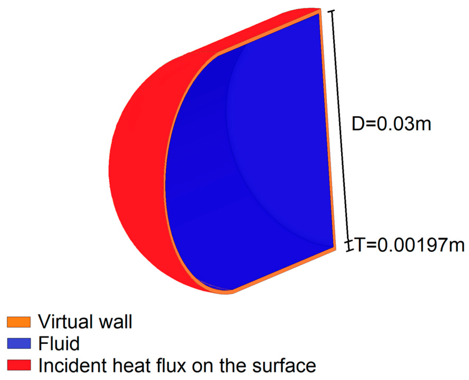
The cylinders were 95% full, with approximately 95% gas purity. The volume was 0.026 m³, the diameter was 0.03 m, and the diameter–length ratio (L/D) equaled 1.33, filled with approximately 13 kg of butane (T1B) and 11 kg of propane (T2P).

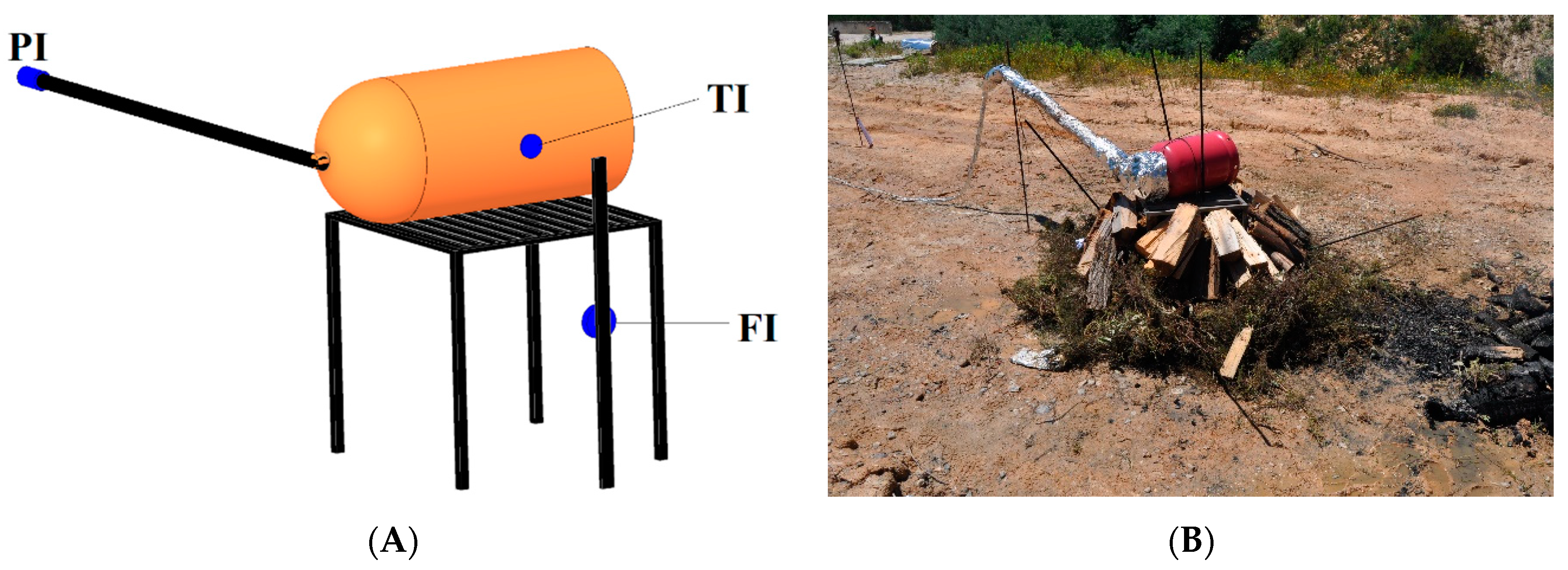
The LPG cylinders were placed in a horizontal position, lying on a support manufactured with steel and placed over fuel (Figure 1). The cylinder was tied through its handles using a steel cable, to avoid movement due to a likely jet fire. The horizontal position was adopted to increase the incident heat flux and engulfment, because otherwise the fuel bed could not keep the cylinder fully engulfed for the entire test period (~10 min). This configuration exposed the cylinder to an extreme scenario. A horizontal position was used in other studies as well [3,15,16].

Forest fuel was used to make the fuel bed. To ensure a similar amount of fuel in both tests, ten pieces of firewood (Pinus pinaster) were used. The firewood pieces’ weight on average was 1.96 ± 0.61 kg, and in each test 60 pieces were used, corresponding to around 120 kg. Finally, 6 kg of dry shrubs were used to start the fire.

A J-type thermocouple (TI 1) was used attached to the cylinder surface at half its height, to register the cylinder surface temperature, in order to feed the fluid’s initial temperature to the CFD setup. The thermocouple uncertainty is ±1.5 °C for temperatures up to 800 °C.

A pressure transducer, model P2VA2 (PI) from HBM, with a range between 0 and 500 bar (1 bar = 1 × 10⁶ Pa) was used. To avoid damage to the pressure transducer from flame impingement, a steel tube of 1.5 m length was coupled to the valve, and the pressure transducer was coupled at the end of the tube (Figure 1). The tube, valve, and PI were protected by aluminum foil and fiberglass, to allow a longer measurement time. The thermocouple and PI were connected to a data logger from Eurotherm model 6100 A.

A total heat flux sensor IHF01 Hukseflux with a calibration uncertainty of ±0.98 × 10⁻⁹ V·(W·m⁻²)⁻¹ was used to measure the heat flux from the flames. It was placed 50 cm from the center of the fuel, to preserve the instrument and the data acquisition system. This sensor was connected to a model 9211 (±80 mV) from National Instruments (NI), and it was plugged into a chassis cDAQ-9174, also from NI. These instruments allowed the continuous measurement of the signal from the sensor with a frequency of 1 Hz [3,17].

The cylinder used in test T1B was equipped with a PRD set to open at 21 bar; and in the test T2P, the PRD opening set was 26 bar.

2.2. Computational Methods

The simulations were performed using Ansys Fluent 2022 R2. The computer used was equipped with a Ryzen 7 5700 U 1.80 GHz processor with a boost of 4.3 GHz.

2.2.1. Domain and Grid

Some assumptions were made in the settings of the CFD model, to reduce the computational cost. Since the main goal of this work was the pressure increment and considering that during the experimental tests the cylinder was fully engulfed by flames, a symmetry condition was applied to reduce the number of cells. Hence, only one half of the cylinder was used [12]. A 3D domain with the same dimensions as the cylinders used in the experimental tests was made to describe the system inside the cylinder. The geometries used for both cases are presented (Figure 2).

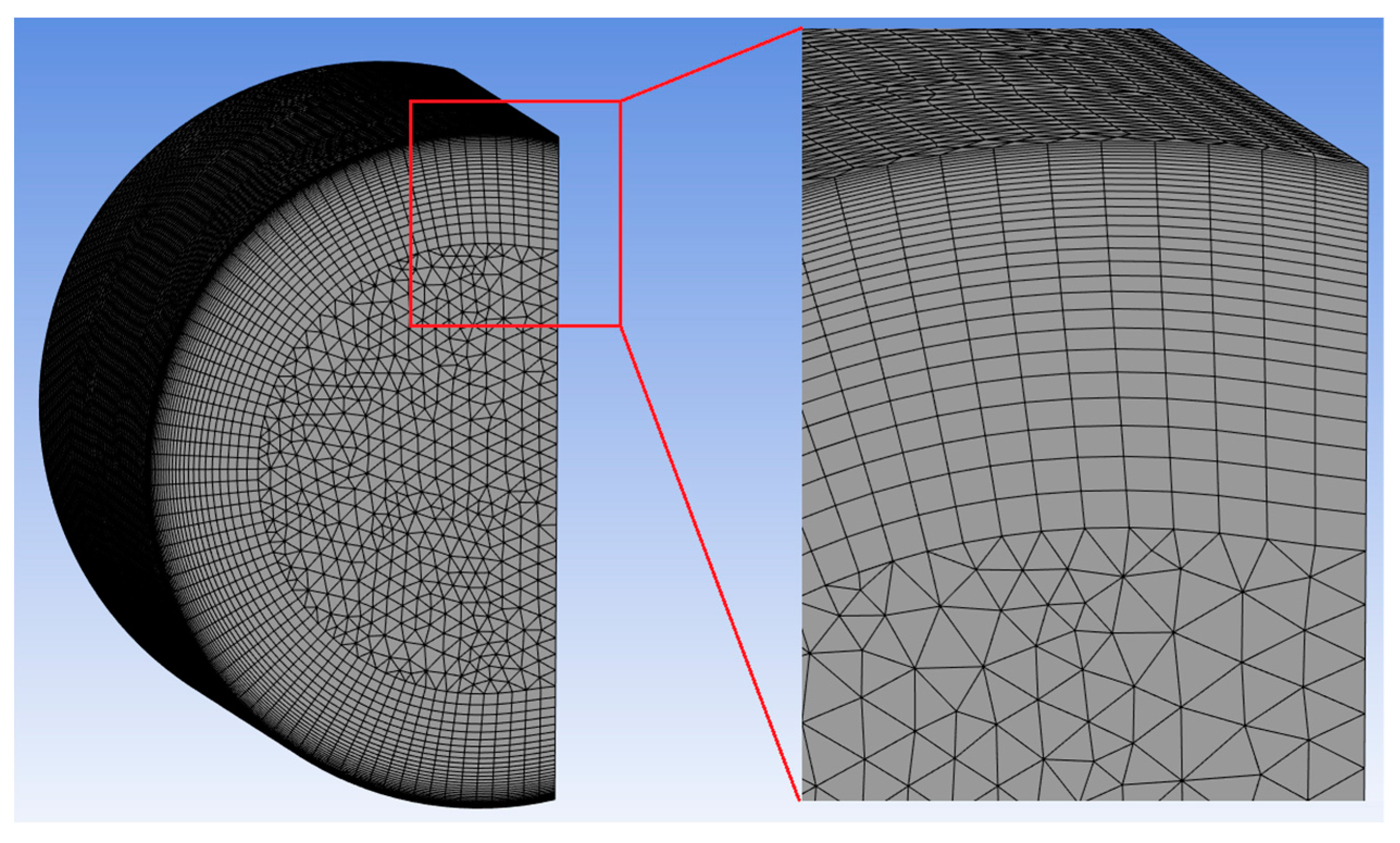
The mesh used in the present manuscript was constructed based on previous work and its proven reliability [12]. In the cited work, the authors simulated some LPG tanks with a capacity of 0.461–11 m³ and performed a grid independence study, which found a discrepancy equal to 0.1 bar between the pressure curves. They used a maximum cell size of 0.03 m and an inflation with 25 layers. Thus, for a tank with a capacity of 0.461 m³, the number of cells was 164,062. In the present paper, the cylinder size was much smaller—0.026 m³. For the mesh generated in the present work, a maximum cell size of 0.013 m was used (around 3 times smaller than the previous size). An inflation with 30 layers and a growth rate equal to 1.1 was applied near the walls, to increase the discretization, since it is in this area that the main wall effects occur: heating, temperature gradient, and convective flow. Thus, this generated 366,228 cells (Figure 3).

Considering that the previous mesh was adequately tested and results were accomplished in good agreement with experimental results, the mesh used in the present paper was denser than those used by other authors. Therefore, performing a new mesh independency test would not bring significant changes.

The quality of the mesh was evaluated based on skewness quality. The closer the skewness is to 0, the better the quality. If it is close to the range of 0.98–1, the mesh is not suitable for use [18]. The averaged skewness on the mesh used was equal to 0.14; therefore, the mesh was suitable for use.

2.2.2. Initial and Boundary Conditions

A uniform incident heat flux was considered over the entire cylinder surface and the pressure was considered the same in the entire cylinder. The pressure and temperature values used to set up the initial conditions in Ansys Fluent were the same as registered in the experimental tests at the moment just before starting the fire. This method aimed to predict the pressure increment up to just before the PRD opens. The filling degree (FD) in both cases was 95%, this value was provided by the trader. Considering the purity of 95% informed by the trader, an approach of 100% was adopted in the numerical method. The incident heat flux on the cylinder surface was set using the average values recorded during the experimental tests (

Table 1. Initial conditions used to set the CFD method.

Simulation	Test	Temperature (°C)	Pressure (Bar)	FD (%)	Dimension	Incident Heat Flux (kW·m−2)
SIMU T1B	T1B	34	5	95	3D	7
SIMU T2P	T2P	38	9.7		3D	5.5

). The tool named Shell Conduction available in Ansys Fluent was used to act like a virtual wall receiving the heat flux. It replaced the cylinder wall (thickness equal to 0.00197 m) and solved the issue of poor-quality mesh in thin geometries. Otherwise, convergence problems may occur or a higher number of cells may be necessary. To set the wall material, a steel available in the Ansys Fluent library was used. The no-slip condition was adopted for the internal wall.

As stated in Table 1, the initial values are counted as Dirichlet conditions. The symmetrical XY plane implies zero velocity gradient in the plane normal direction, z,

$$\overrightarrow{v}·\overrightarrow{n}=0$$

(1)

Moreover, the pressure gradient in the circumferential direction was neglected.

2.2.3. Governing Equations and Models

The CFD model was computed using the following governing equations. For energy, the equation is

$$\frac{\partial }{\partial t}\left(\rho E\right)+\nabla ·\left[\overrightarrow{v}\left(\rho E+p\right)\right]=-\nabla \mathrm{p}+-\nabla ·\left(k_{eff}\nabla \mathrm{T}\right)+H_{vap}\left(\dot{m_{v\to l}}-\dot{ m_{l\to v}}\right)$$

(2)

where E is the two-phase averaged specific energy, $k_{eff}$ is the effective thermal conductivity, $H_{vap}$ is the heat of vaporization, $\overrightarrow{v}$ is the averaged velocity, ρ is density, and T is temperature.

The equation for momentum is as follows:

$$\frac{\partial }{\partial t}\left(\rho \overrightarrow{v}\right)+\nabla ·\left(\rho \overrightarrow{v}\overrightarrow{v}\right)=-\nabla \mathrm{p}+\nabla \left[\mu \left(\nabla \overrightarrow{v}+\nabla {\overrightarrow{v}}^T\right)\right]+\rho \overrightarrow{g}+\overrightarrow{F}$$

(3)

where p is the averaged pressure, $\overrightarrow{F}$ is the force vector (the gravitational body force and external body forces), $\overrightarrow{g}$ is the gravity acceleration, $\rho$ is the two-phase volume fraction averaged density, and $\mu$ is the two-phase averaged viscosity.

Due to stored LPG being a two-phase system, a multiphase model must be adopted. The widely used volume of fluid (VoF) model [10,11,12,14,19], available in the Ansys Fluent library, was adopted. An evaporation–condensation mechanism based on the Lee model was used. VoF uses an equation for each phase, and it finds the volume fraction for each cell of the domain at each time step. Thus, the percentage of gas and liquid is found through the summing of all cells. It is recommended that the gas phase should be set as the primary phase [20]. For the secondary phase, the equation is as follows:

$$\frac{\partial }{\partial t}\left({\alpha }_l{\rho }_l\right)+\nabla \left({\alpha }_l{\rho }_l\overrightarrow{v_l}\right)=\dot{ m_{v\to l}}-\dot{ m_{l\to v}}$$

(4)

and the volume fraction of the primary phase:

$${\alpha }_v=1-{\alpha }_l$$

(5)

where $\dot{m_{v\to l}}$ and $\dot{ m_{l\to v}}$ are the mass transfer from the vapor phase to the liquid phase and from liquid to vapor, respectively; l is liquid and v is vapor; and α is the volume fraction in a cell.

For turbulence, the k-ω-SST (k-ω-Shear Stress Transport) was adopted. It is based on RANS (Reynolds Average Navier–Stokes simulation). The k-ω-SST is focused on the averaged flow and has two transport equations: the transport equation for the turbulence kinetic energy (k) and another for the specific dissipation rate (ω). The k-ω-SST also considers the turbulent viscosity for the shear stress transport, thus performing better than the k-Ɛ model in the boundary layer. The k-ω-SST was adopted by reason of being better than k-Ɛ at securing the wall effects, recirculation region, and for cases with pressure gradients, making it more appropriate for the case of study. Furthermore, the k-ω-SST was used by other authors [11,12,13,14]. Therefore, k-ω-SST can be applied to a large range of flows. For free shear layers that model was the standard k-Ɛ [21,22].

The equation for the turbulence kinetic energy:

$$\frac{\partial }{\partial t}\left(\rho k\right)+\frac{\partial }{\partial x_j}\left(\rho k{u}_j\right)=\frac{\partial }{\partial x_j}\left[{\mathsf{\Gamma }}_k\frac{\partial k}{\partial x_j}\right]+G_k+G_b-Y_k+S_k$$

(6)

and for specific dissipation rate:

$$\frac{\partial }{\partial t}\left(\rho \omega \right)+\frac{\partial }{\partial x_j}\left(\rho \omega u_j\right)=\frac{\partial }{\partial x_j}\left[{\mathsf{\Gamma }}_{\omega }\frac{\partial \omega }{\partial x_j}\right]+G_{\omega }-Y_{\omega }+D_{\omega }+G_{\omega b}+S_{\omega }$$

(7)

where G_k represents the generation of turbulence kinetic energy due to mean velocity gradients; G_ω represents the generation of specific dissipation rate; Y_k and Y_ω represent the dissipation of k and ω due to turbulence; D_ω represents the cross-diffusion term; S_k and S_ω are user-defined source terms; G_b is the turbulence generation due to buoyancy; G_bω is the buoyancy term in the ω-equation; u is the velocity; t is time; and Γ_ω and Γ_k are the effective diffusivities for k and ω.

To model the gas density, liquid, and vapor phases in Ansys Fluent, the Peng–Robinson equation can provide a good agreement for liquid–vapor equilibrium close to the critical point, once it has imbedded parameters as a function of the critical pressure and temperature.

$$P=\frac{RT}{V-b}-\frac{a_c{\alpha }_p}{V\left(V+b\right)+b\left(V-b\right)}$$

(8)

$$a_c=\frac{0.45727R^2{T}_c^2}{P_c}$$

(9a)

$$b=\frac{0.07780R{T}_c}{P_c}$$

(9b)

$${\alpha }_p={\left[1+f_w\left(1-T_r^{\frac{1}{2}}\right)\right]}^2$$

(9c)

$$f_w=0.37464+1.5422w-0.2699w^{2 }$$

(9d)

$$T_R=\frac{T}{T_c} P_R=\frac{P}{P_c}$$

(9e)

where T_r is the reduced temperature, $w$ is the acentric factor; P_c and T_c are the critical pressure and temperature, respectively; and f is fugacity.

2.2.4. Solution Methods

A pressure-based solver and a first-order scheme with a time-step equal to 0.005 s were adopted in both cases. The convergence criterions used were for scaled residuals, lower than 10⁻³; and for the energy equation 10⁻⁶.

Table 2. Discretization schemes used in both simulations.

Discretization Scheme
Pressure–Velocity Coupling	SIMPLEC
Pressure	PRESTO!
Density	Second order upwind
Momentum	Second order upwind
Turbulence (k e ω)	Second order upwind
Volume fraction	Geo-reconstruction
Energy	Second order upwind

and

Table 3. Relaxations factors used in both simulations.

Variable	Relaxation Factor
Pressure	0.3
Density	1
Body forces	0.8
Momentum	0.7
Vaporization mass	1
Turbulent kinetic energy	0.8
Turbulent viscosity	1
Turbulent dissipation rate	0.8
Energy	1

summarize the spatial discretization schemes and relaxation factors adopted.

2.2.5. Validation

The CFD methods were compared to the experimental results. Due to the flames from forest fuels taking some time to fully develop, the same methodology as adopted previously in [12] was used. Thus, the delay of flames and the start of the simulation were set consistently.

3. Results

3.1. The Pressure Increment

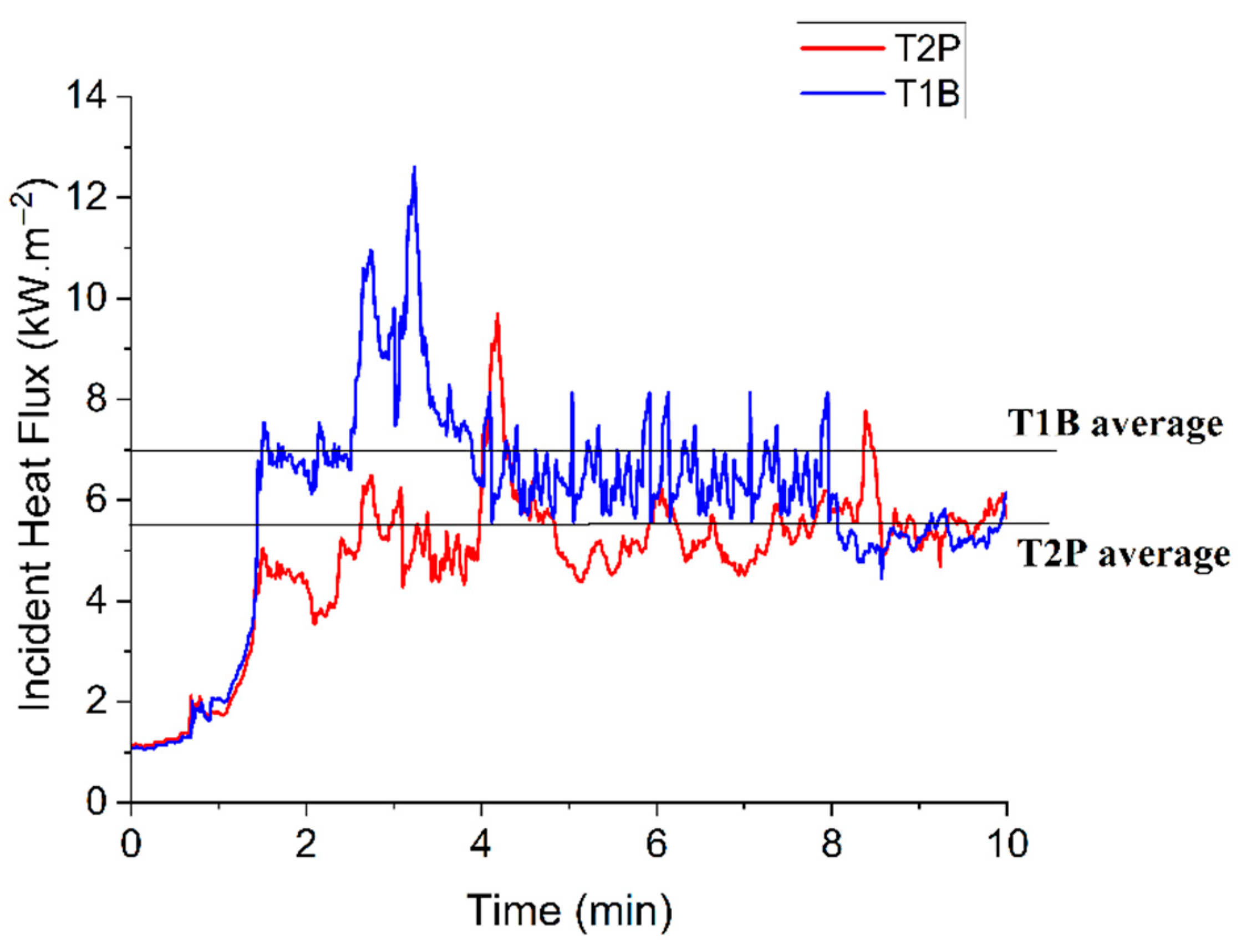
Figure 4 presents the incident heat flux for tests T1B and T2P, and their averages, which were used to set the heat flux in the CFD setup. The flames took around 2 min to become fully developed in tests T1B and T2P.

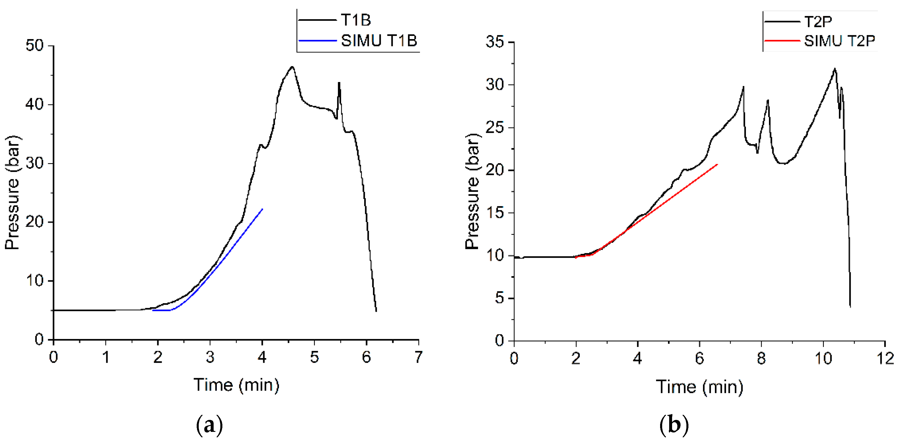
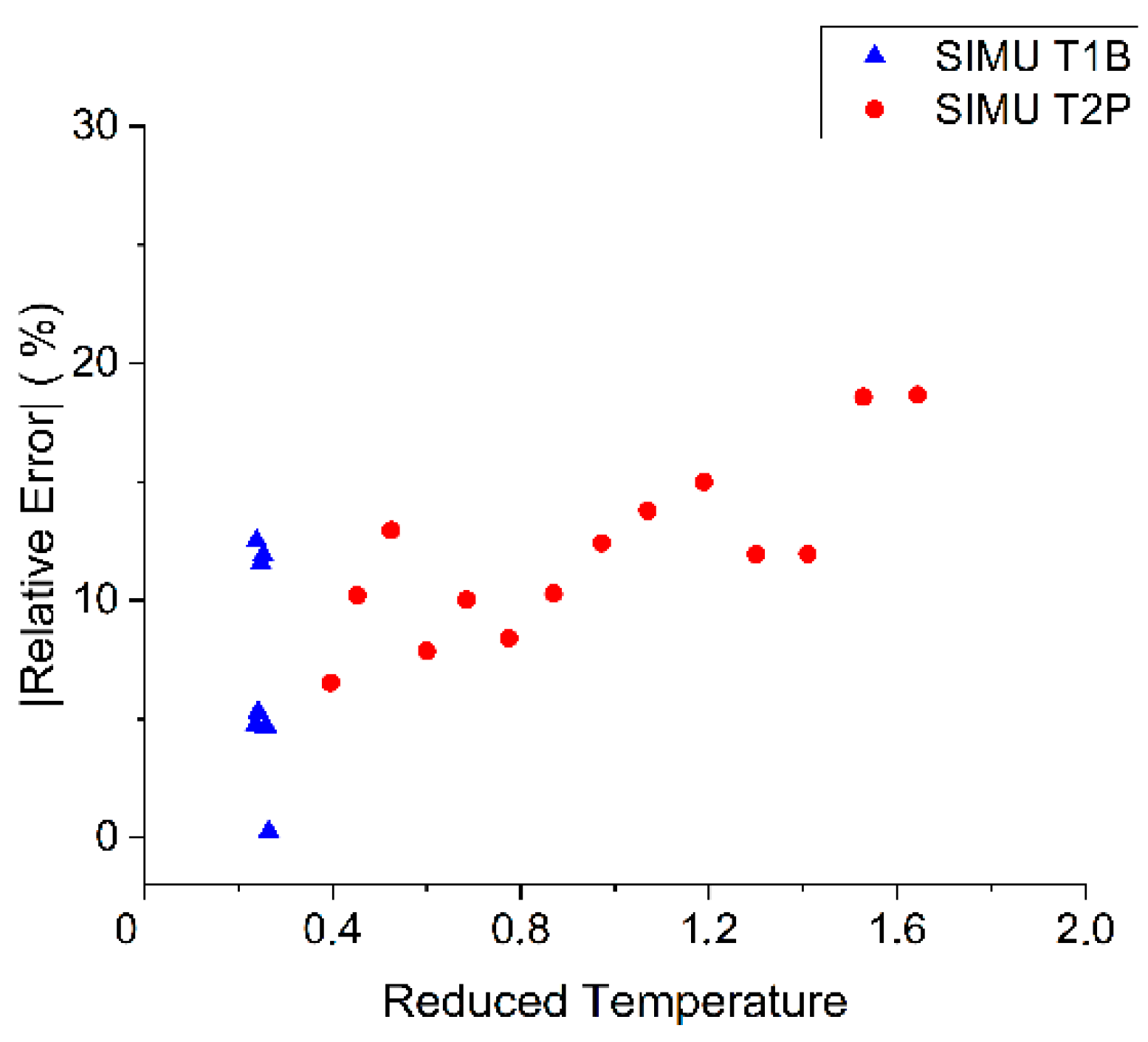
The SIMU T1B had a good agreement between the simulated and experimental pressure curves until 4 min, with a relative error ≤ 12.3% (Figure 5a). However, after that, the relative error increased. For SIMU T2P (Figure 5b), a similar behavior to SIMU T1B could be noted. Until five minutes, the relative error was ≤9%, at 6 min it was 18%; after that, the error increased significantly.

The error increment between the simulated and experimental pressure curves after some minutes could be related to the high fluid temperatures. For SIMU T1B, at three minutes, a reduced temperature (TR) of 0.22 was found through the averaged internal temperature; and after four minutes, the reduced temperature was 0.3. A similar behavior was seen in SIMU T2P; before five minutes, the reduced temperature was up to 1.1, but then it increased to 1.7 at 6 min. This suggests a relation between the error and the temperature. This behavior was more pronounced for propane, and its heating rate was higher than butane. In addition, a relevant overprediction for the temperature of the vapor phase was mentioned [12].

The high temperature and its overprediction hindered the pressure increment prediction, because it increased the distance from the critical point, which is the border prediction for a cubic equation of state such as the Peng–Robinson. Even under an overpredicted temperature, the results showed that the CFD model had a good agreement with the experiment, but this was better for butane than propane.

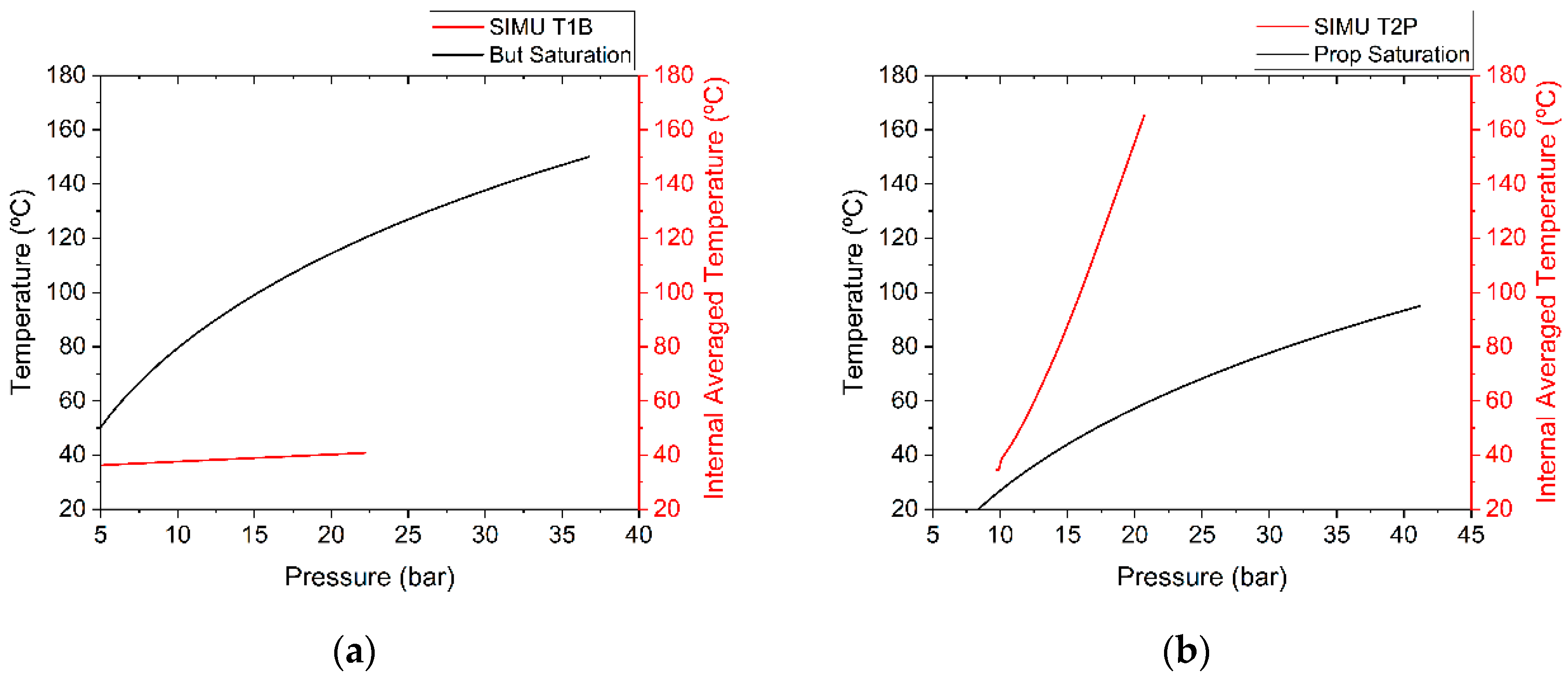
One way to show the temperature overprediction was to compare the simulated values of pressure and temperature with the vapor–liquid equilibrium (VLE) curve. This comparison does not provide an exact overprediction value, but it shows that there was an overprediction. The low accuracy was because the VLE did not consider the test dynamics and CFD; the CFD method takes into account several items that a saturation curve [23] does not.

Figure 6 presents the pressure and temperature of the CFD method and the VLE curve for each case. It can be noted that, at 20 bar for the saturation curve, the respective temperature for propane was 60 °C. However, for the SIMU T2P curve, at the same pressure, the temperature was approximately 170 °C. Thus, there was a relevant overprediction, and the temperature increased faster than the pressure. In Figure 6, it can also be noted that this trend was more noticeable for propane than butane. Therefore, as seen in both cases studied, the increment of the reduced temperature caused an error increment between the experimental and CFD pressure curves (Figure 7).

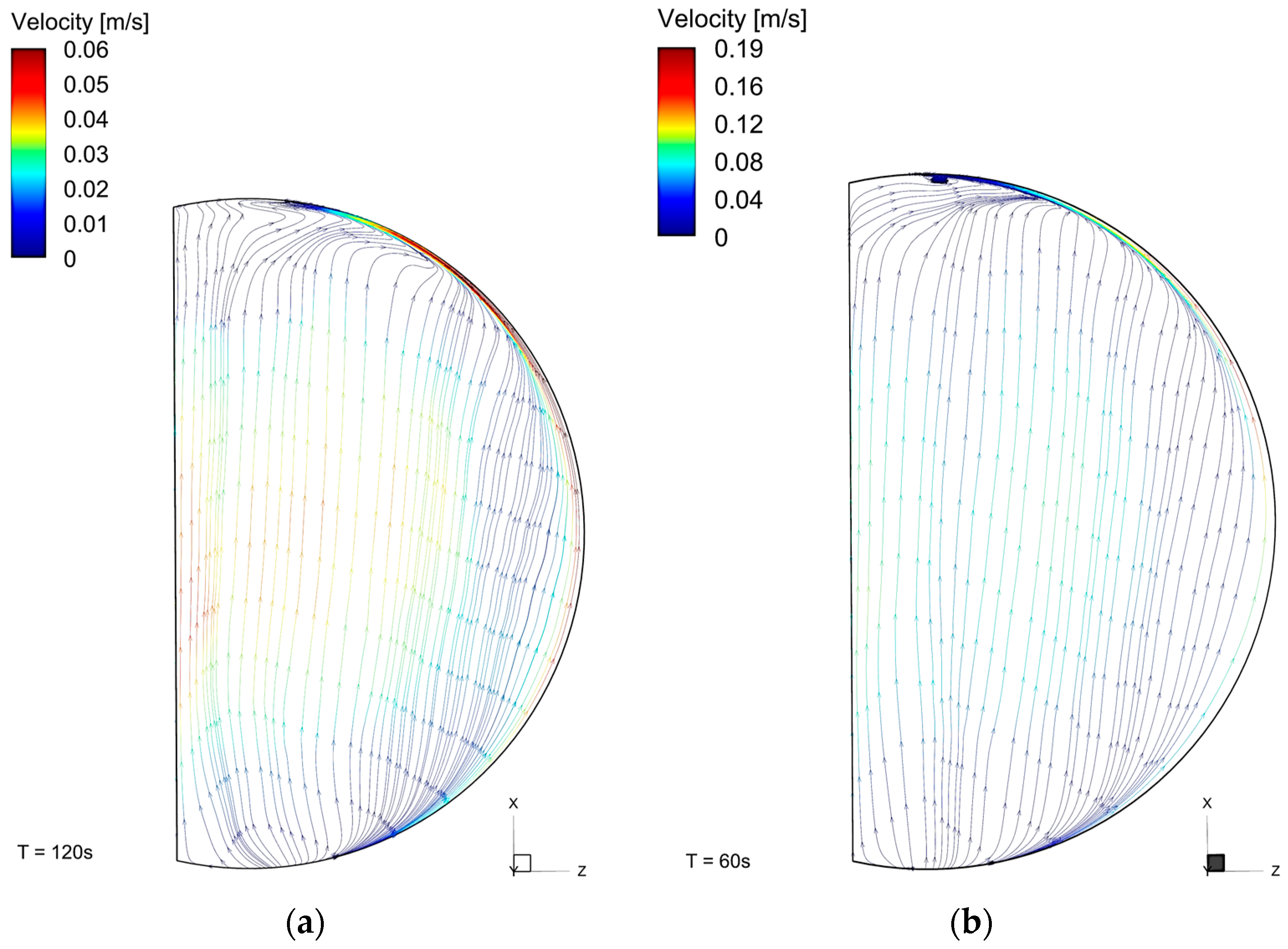
3.2. Flow and Temperature Profile near Walls

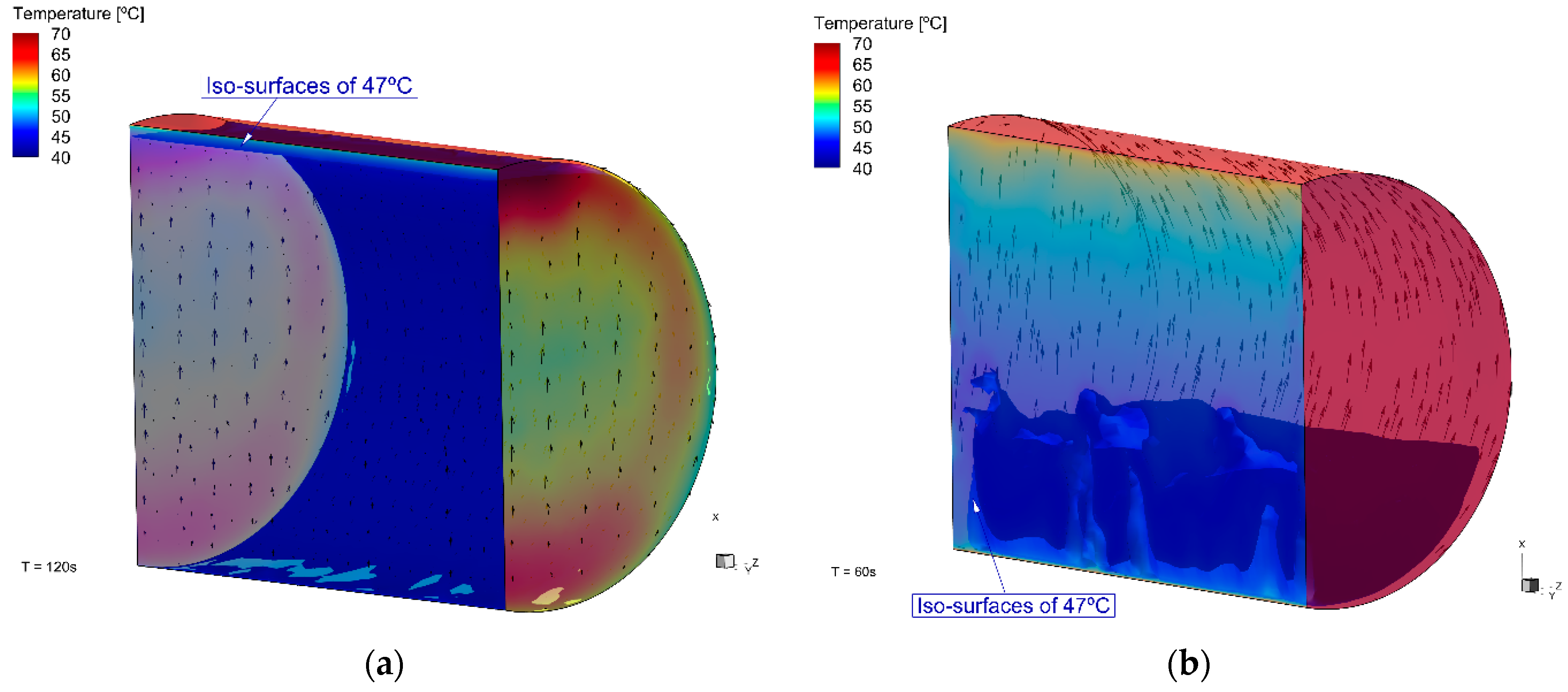
The flow was influenced by the wall temperature, and there was a thermal gradient between the walls and the center of the cylinder (Figure 8). The zones with the highest temperatures, near the walls and the top, were the zones with the highest fluid velocities (Figure 9). The flow was upwards near the side walls and it dropped down near the cylinder’s center. The velocities near the walls were up to 0.05 m·s⁻¹ for butane (T1C); and for propane, this was higher, up to 0.18 m·s⁻¹. In addition, the recirculation zones in the T2P case can be noted.

Propane had a faster warming than butane, due to a lower specific heat at a constant volume (up to 66.9 °C); however, the difference was not large. Despite these thermal properties, the faster temperature increment of propane can be noted in Figure 8, from the simulation at different times (120 s for butane and 60 s for propane). Even in the T1B case at 120 s, which means a longer warming time, the temperature in T2P at 60 s was higher. This also confirms the temperature overprediction for the lighter fluid.

4. Discussion

The results show that the numerical methods had a reasonable agreement with the experimental data, mainly at low reduced temperatures. In addition, propane, which is a lighter alkane than butane, presented a higher temperature overprediction at higher reduced temperatures, as well as a higher error. Furthermore, the comparison between propane and butane revealed that the CFD method fit better with a heavier fluid; even in test T1B with butane, where the cylinder was under an incident heat flux around 30% higher than in test T2P with propane. The reservoirs used in this study could store a small amount of fluid, so for cases with a larger amount of LPG, the prediction for propane could work for a longer prediction time, as more fluid can absorb more energy.

It was seen that higher errors were found from the third minute of simulation. At this moment, the temperature was much higher than the critical temperature. The results showed a trend in the error increment associated with the reduced temperature increment. For a reduced temperature up to 1.7, which for propane represents around 163 °C, the relative errors between experimental and CFD results was up to 18%.

The relative errors found in this work, up to 18%, are similar to those found in previous studies, in which tanks with a capacity up to 125 m³ were assessed and errors up to 23% were found [8,12].

Various reasons may have contributed to these errors and to the limitations of the method. The main reasons are listed as follows:

• The Peng–Robinson parameters available in the code do not include the supercritical data for a two-phase case. Thus, the greater the distance from the critical point, the greater the error;
• The cubic equation of state models can be used to solve problems in the gas, liquid, and supercritical fluid regimes. These models are not available for the two-phase region under the phase domain [20];
• Other thermodynamic models based on statistical thermodynamics, for instance, the SAFT equation [24] that presents better results in the supercritical range, can be tested in further works through a user-defined function (UDF);
• The fluid in the cylinder was not pure. This was due to the high degree of purity (95%). LPG does not have water or other polar fluids in the mix. In fact, minor fractions of other fluids can behave differently than propane and butane under the liquid–vapor equilibrium domain and in a supercritical state. Thus, some fractions of the fluid can behave as a supercritical fluid whilst others are not supercritical;
• The propane and butane liquified had traces of heavy petroleum and noncondensing;
• The experimental tests used a forest fuel, which did not have a uniform heat flux during the duration of the tests. Thus, if a gas burner was used, the relative error may have been lower.

The processing required a very long time. This is an issue to be overcome. In this study, the time process for both cases was around 3.5 h for processing 1 s of the simulation.

5. Conclusions

This study presented an assessment regarding the pressure increment prediction of LPG under fire engulfment through CFD. The results obtained showed that for lighter alkanes, the error increment between the experimental and simulated pressure curves was greater than for the heavier alkanes. In addition, there was a trend of higher errors at higher reduced temperatures, which may have been due to the code overpredicting the temperature.

The CFD method can be useful for cases in which the reduced temperature is up to 1.7, which has shown relative errors up to 18%. It can be applied for various cases related to safety, such as vessels heated by a jet fire or a pool fire, when the incident heat flux on the equipment wall can be estimated.

The processing time is high; however, by utilizing a powerful CPU, the processing time can be decreased, and the license acquisition permit dedicates more cores for processing.

References

- Jung, S.; Woo, J.; Kang, C. Analysis of Severe Industrial Accidents Caused by Hazardous Chemicals in South Korea from January 2008 to June 2018. Saf. Sci. 2020, 124, 104580. [Google Scholar] [CrossRef]
- Xiang, Y.; Wang, Z.; Zhang, C.; Chen, X.; Long, E. Statistical Analyasis of Major Industrial Accidents in China from 2000 to 2020. Eng. Fail. Anal. 2022, 141, 106632. [Google Scholar] [CrossRef]
- Barbosa, T.F.; Reis, L.; Raposo, J.; Rodrigues, T.; Viegas, D.X. LPG Stored at the Wildland–Urban Interface: Recent Events and the Effects of Jet Fires and BLEVE. Int. J. Wildl. Fire 2023, 32, 388–402. [Google Scholar] [CrossRef]
- Manu, C.C.; Birk, A.M.; Kim, I.Y. Stress Rupture Predictions of Pressure Vessels Exposed to Fully Engulfing and Local Impingement Accidental Fire Heat Loads. Eng. Fail. Anal. 2009, 16, 1141–1152. [Google Scholar] [CrossRef]
- Lowesmith, B.J.; Hankinson, G.; Acton, M.R.; Chamberlain, G. An Overview of the Nature of Hydrocarbon Jet Fire Hazards in the Oil and Gas Industry and a Simplified Approach to Assessing the Hazards. Process Saf. Environ. Prot. 2007, 85, 207–220. [Google Scholar] [CrossRef]
- Palacios, A.; García, W.; Rengel, B. Flame Shapes and Thermal Fluxes for an Extensive Range of Horizontal Jet Flames. Fuel 2020, 279, 118328. [Google Scholar] [CrossRef]
- Shen, R.; Jiao, Z.; Parker, T.; Sun, Y.; Wang, Q. Recent Application of Computational Fluid Dynamics (CFD) in Process Safety and Loss Prevention: A Review. J. Loss Prev. Process Ind. 2020, 67, 104252. [Google Scholar] [CrossRef]
- D’Aulisa, A.; Tugnoli, A.; Cozzani, V.; Landucci, G.; Birk, A.M. CFD Modeling of LPG Vessels under Fire Exposure Conditions. AIChE J. 2014, 60, 4292–4305. [Google Scholar] [CrossRef]
- D’Aulisa, A.; Simone, D.; Landucci, G.; Tugnoli, A.; Cozzani, V.; Birk, M. Numerical Simulation of Tanks Containing Pressurized Gas Exposed to Accidental Fires: Evaluation of the Transient Heat Up. Chem. Eng. Trans. 2014, 36, 241–246. [Google Scholar]
- Landucci, G.; D’Aulisa, A.; Tugnoli, A.; Cozzani, V.; Birk, A.M. Modeling Heat Transfer and Pressure Build-up in LPG Vessels Exposed to Fires. Int. J. Therm. Sci. 2016, 104, 228–244. [Google Scholar] [CrossRef]
- Scarponi, G.E.; Landucci, G.; Birk, A.M.; Cozzani, V. LPG Vessels Exposed to Fire: Scale Effects on Pressure Build-Up. J. Loss Prev. Process Ind. 2018, 56, 342–358. [Google Scholar] [CrossRef]
- Scarponi, G.E.; Landucci, G.; Birk, A.M.; Cozzani, V. An Innovative Three-Dimensional Approach for the Simulation of Pressure Vessels Exposed to Fire. J. Loss Prev. Process Ind. 2019, 61, 160–173. [Google Scholar] [CrossRef]
- Scarponi, G.E.; Landucci, G.; Heymes, F.; Cozzani, V. Experimental and Numerical Study of the Behavior of LPG Tanks Exposed to Wildland Fires. Process Saf. Environ. Prot. 2018, 114, 251–270. [Google Scholar] [CrossRef]
- Scarponi, G.E.; Landucci, G.; Birk, A.M.; Cozzani, V. Three Dimensional CFD Simulation of LPG Tanks Exposed to Partially Engulfing Pool Fires. Process Saf. Environ. Prot. 2021, 150, 385–399. [Google Scholar] [CrossRef]
- Tschirschwitz, R.; Krentel, D.; Kluge, M.; Askar, E.; Habib, K.; Kohlhoff, H.; Krüger, S.; Neumann, P.P.; Storm, S.U.; Rudolph, M.; et al. Experimental Investigation of Consequences of LPG Vehicle Tank Failure under Fire Conditions. J. Loss Prev. Process Ind. 2018, 56, 278–288. [Google Scholar] [CrossRef]
- Tschirschwitz, R.; Krentel, D.; Kluge, M.; Askar, E.; Habib, K.; Kohlhoff, H.; Neumann, P.P.; Storm, S.U.; Rudolph, M.; Schoppa, A.; et al. Mobile Gas Cylinders in Fire: Consequences in Case of Failure. Fire Saf. J. 2017, 91, 989–996. [Google Scholar] [CrossRef]
- Barbosa, T.F.; Reis, L.; Raposo, J.; Viegas, D.X. A Protection for LPG Domestic Cylinders at Wildland-Urban Interface Fire. Fire 2022, 5, 63. [Google Scholar] [CrossRef]
- Park, H.; Lee, J.; Lim, J.; Cho, H.; Kim, J. Optimal Operating Strategy of Ash Deposit Removal System to Maximize Boiler Efficiency Using CFD and a Thermal Transfer Efficiency Model. J. Ind. Eng. Chem. 2022, 110, 301–317. [Google Scholar] [CrossRef]
- Bi, M.S.; Ren, J.J.; Zhao, B.; Che, W. Effect of Fire Engulfment on Thermal Response of LPG Tanks. J. Hazard. Mater. 2011, 192, 874–879. [Google Scholar] [CrossRef]
- ANSYS Inc. Ansys Fluent User’s Guide; Release 20; ANSYS Inc.: Canonsburg, PA, USA, 2022. [Google Scholar]
- ANSYS Inc. Ansys Fluent Theory Guide; Release 20; ANSYS Inc.: Canonsburg, PA, USA, 2022. [Google Scholar]
- Menter, F.R. Two-Equation Eddy-Viscosity Turbulence Models for Engineering Applications. AIAA J. 1994, 32, 1598–1605. [Google Scholar] [CrossRef]
- National Institute of Standards and Technology Thermophysical Properties of Fluid Systems—NIST Chemistry. Available online: https://webbook.nist.gov/chemistry/fluid/ (accessed on 7 April 2022).
- Gross, J.; Sadowski, G. Reply to Comment on “Perturbed-Chain SAFT: An Equation of State Based on a Perturbation Theory for Chain Molecules”. Ind. Eng. Chem. Res. 2001, 40, 1244–1260. [Google Scholar] [CrossRef]