
Droplet Based Estimation of Viscosity of Water–PVP Solutions Using Convolutional Neural Networks

 ,
,  , and
, and
Abstract
1. Introduction
2. Materials and Methods
2.1. Materials
2.2. Measurement Setup
2.3. Methods
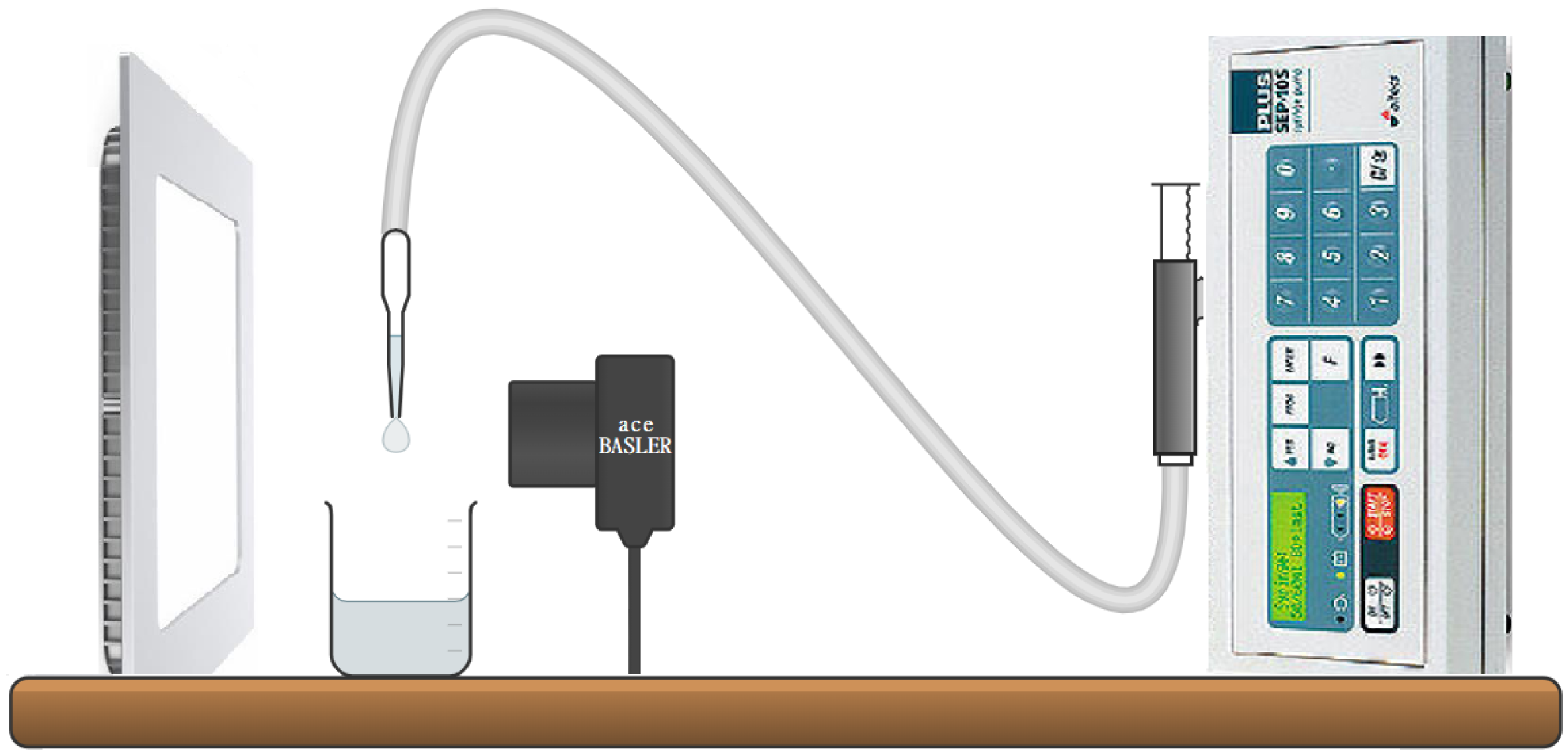
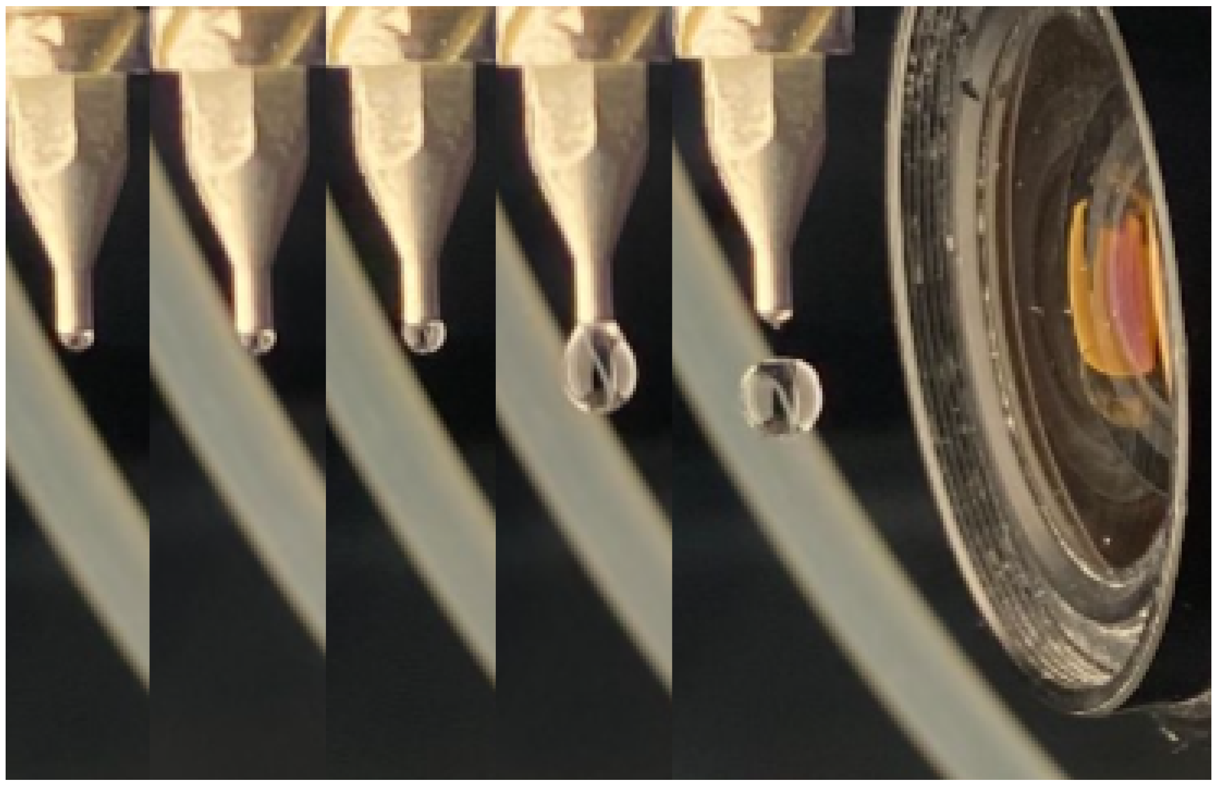
2.3.1. Experimental Setup
2.3.2. Viscosity Measurement
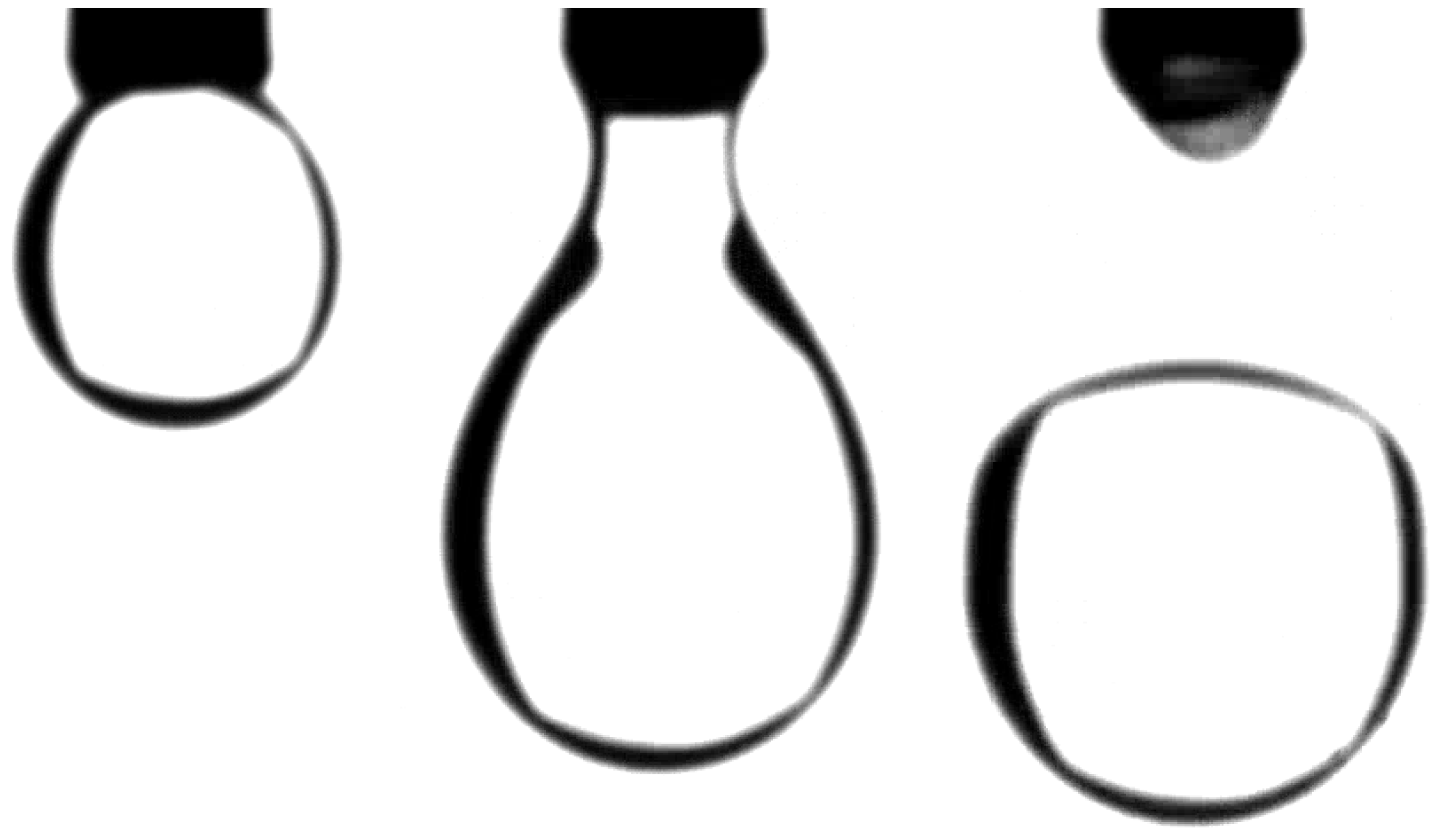
2.3.3. Data Analysis
2.3.4. Convolutional Neural Networks
2.3.5. Evaluation Measurement
- Mean squared error (MSE): The MSE calculates the average of the squared differences between the predicted and actual values. It is the metric used by the proposed models for the loss function.where n is the number of samples in the dataset, and and represent the predicted and actual values for the ith sample, respectively.
- Mean absolute error (MAE): This metric calculates the average absolute difference between the predicted and actual values. The MAE is a good metric to use when the dataset has a large number of outliers because it is less sensitive to outliers than other metrics such as MSE. Since our data consist of images that are quite similar to the naked eye but might hide some outliers, it would be important to check the MAE.where n is the number of samples in the dataset, and and represent the predicted and actual values for the ith sample, respectively.
- R2 score (coefficient of determination): The is a metric that measures the proportion of the variance in the dependent variable that is predictable from the independent variables. It provides an indication of how well the model fits the data. The score ranges from 0 to 1, with 1 indicating a perfect fit.where is the variance of the actual values.
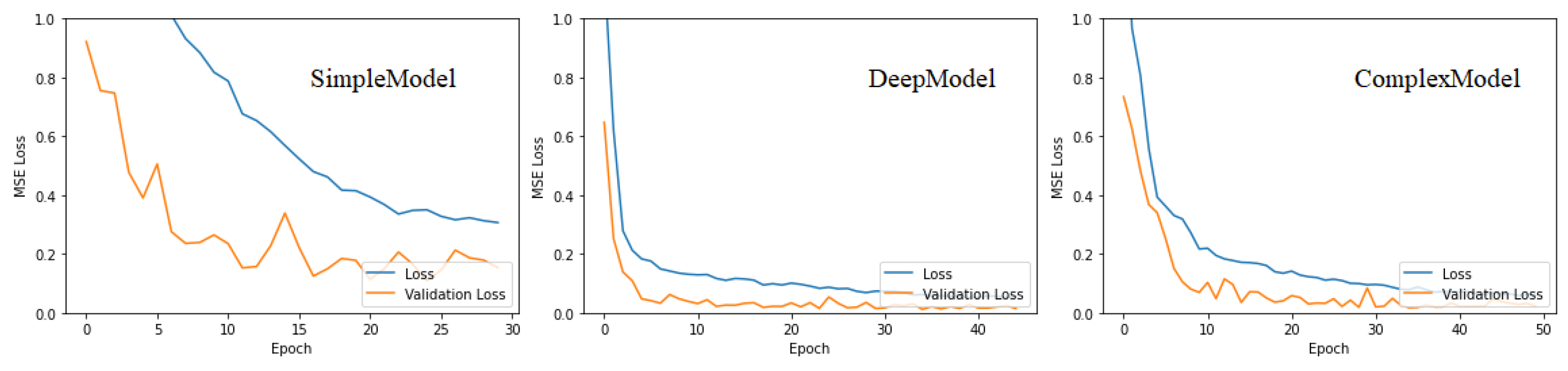
3. Results and Discussion
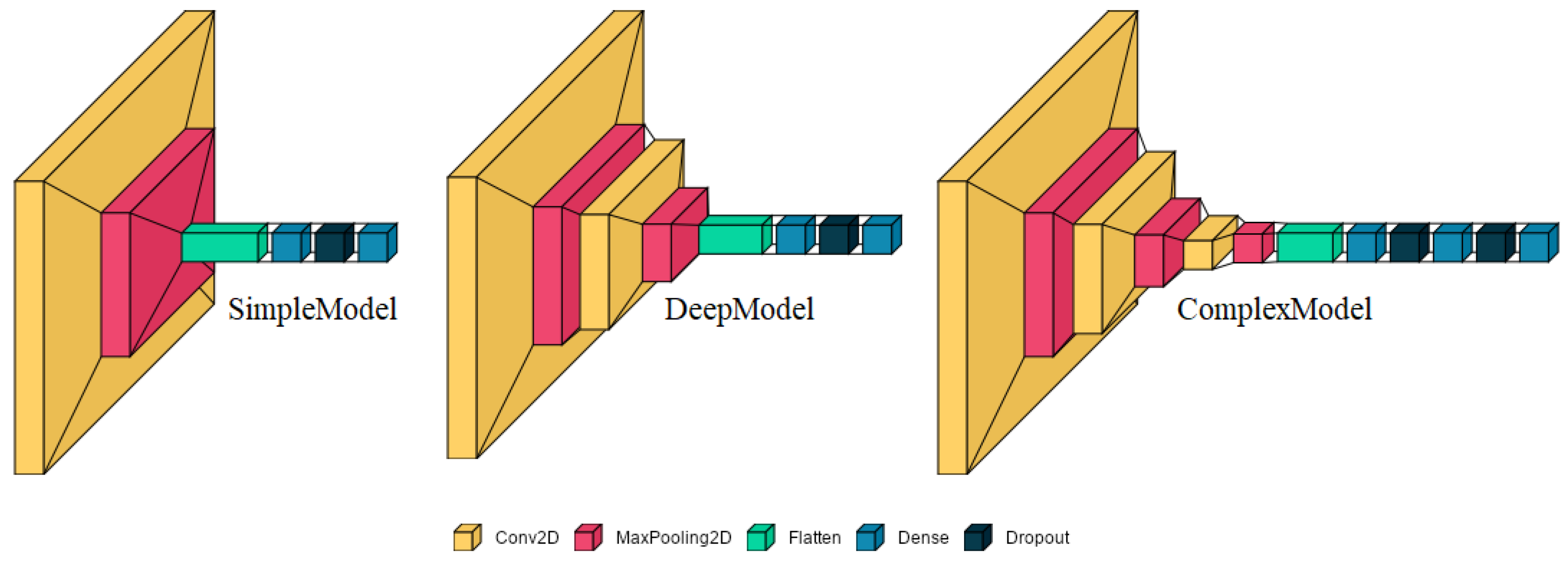
- SimpleModel: The SimpleModel has a basic architecture, which consists of 1 convolutional layer with 32 filters of size (3, 3), followed by a max-pooling layer of size (2, 2), a flatten layer, 2 dense layers of sizes 64 and 1, respectively, and a dropout layer with a rate of 0.5. The input shape of the SimpleModel is (91, 53, 3), which represents the size of the input droplet images.
- DeepModel. This model architecture is more complex than the SimpleModel, consisting of two convolutional layers with 32 and 64 filters of sizes (5, 5) and (5, 5), respectively, followed by 2 max-pooling layers of size (2,2), a flatten layer, 2 dense layers of sizes 128 and 1, respectively, and a dropout layer with a rate of 0.5. The input shape of the DeepModel is also (91, 53, 3).
- ComplexModel. This model architecture is the most complex of the 3 models and includes 3 convolutional layers with 32, 64, and 64 filters of sizes (7, 7), (7, 7), and (7, 7), respectively, followed by 3 max-pooling layers of size (2, 2), a flatten layer, 3 dense layers of sizes 128, 64, and 1, respectively, and 2 dropout layers with a rate of 0.5. The input shape of the ComplexModel is also (91, 53, 3).
4. Conclusions
Author Contributions
Funding
Institutional Review Board Statement
Informed Consent Statement
Data Availability Statement
Conflicts of Interest
Abbreviations
| CNN | Convolutional Neural Network |
| PVP | Polyvinylpyrrolidone |
References
- Viswanath, D.S.; Ghosh, T.K.; Prasad, D.H.; Dutt, N.V.; Rani, K.Y. Viscosity of Liquids: Theory, Estimation, Experiment, and Data; Springer Science & Business Media: Dordrecht, The Netherlands, 2007. [Google Scholar]
- Toropainen, E.; Fraser-Miller, S.J.; Novakovic, D.; Del Amo, E.M.; Vellonen, K.S.; Ruponen, M.; Viitala, T.; Korhonen, O.; Auriola, S.; Hellinen, L.; et al. Biopharmaceutics of topical ophthalmic suspensions: Importance of viscosity and particle size in ocular absorption of indomethacin. Pharmaceutics 2021, 13, 452. [Google Scholar] [CrossRef] [PubMed]
- Lokhande, A.B.; Mishra, S.; Kulkarni, R.D.; Naik, J.B. Influence of different viscosity grade ethylcellulose polymers on encapsulation and in vitro release study of drug loaded nanoparticles. J. Pharm. Res. 2013, 7, 414–420. [Google Scholar] [CrossRef]
- Bourne, M. Food Texture and Viscosity: Concept and Measurement; Elsevier: Amsterdam, The Netherlands, 2002. [Google Scholar]
- Nunes, V.M.; Lourenço, M.J.; Santos, F.J.; Nieto de Castro, C.A. Importance of accurate data on viscosity and thermal conductivity in molten salts applications. J. Chem. Eng. Data 2003, 48, 446–450. [Google Scholar] [CrossRef]
- Rashid, B.; Bal, A.L.; Williams, G.J.; Muggeridge, A.H. Using vorticity to quantify the relative importance of heterogeneity, viscosity ratio, gravity and diffusion on oil recovery. Comput. Geosci. 2012, 16, 409–422. [Google Scholar] [CrossRef]
- Hemmati-Sarapardeh, A.; Shokrollahi, A.; Tatar, A.; Gharagheizi, F.; Mohammadi, A.H.; Naseri, A. Reservoir oil viscosity determination using a rigorous approach. Fuel 2014, 116, 39–48. [Google Scholar] [CrossRef]
- Brooks, R.; Dinsdale, A.; Quested, P. The measurement of viscosity of alloys—A review of methods, data and models. Meas. Sci. Technol. 2005, 16, 354. [Google Scholar] [CrossRef]
- Zhao, H.; Memon, A.; Gao, J.; Taylor, S.D.; Sieben, D.; Ratulowski, J.; Alboudwarej, H.; Pappas, J.; Creek, J. Heavy oil viscosity measurements: Best practices and guidelines. Energy Fuels 2016, 30, 5277–5290. [Google Scholar] [CrossRef]
- Caponi, M.; Cox, A.; Misra, S. Viscosity prediction using image processing and supervised learning. Fuel 2023, 339, 127320. [Google Scholar] [CrossRef]
- Zhang, T.; Cao, D.; Feng, X.; Zhu, J.; Lu, X.; Mu, L.; Qian, H. Machine learning prediction of bio-oil characteristics quantitatively relating to biomass compositions and pyrolysis conditions. Fuel 2022, 312, 122812. [Google Scholar] [CrossRef]
- Cengiz, E.; Babagiray, M.; Aysal, F.E.; Aksoy, F. Kinematic viscosity estimation of fuel oil with comparison of machine learning methods. Fuel 2022, 316, 123422. [Google Scholar] [CrossRef]
- Rahmanifard, H.; Maroufi, P.; Alimohamadi, H.; Plaksina, T.; Gates, I. The application of supervised machine learning techniques for multivariate modelling of gas component viscosity: A comparative study. Fuel 2021, 285, 119146. [Google Scholar] [CrossRef]
- Afrand, M.; Najafabadi, K.N.; Sina, N.; Safaei, M.R.; Kherbeet, A.S.; Wongwises, S.; Dahari, M. Prediction of dynamic viscosity of a hybrid nano-lubricant by an optimal artificial neural network. Int. Commun. Heat Mass Transf. 2016, 76, 209–214. [Google Scholar] [CrossRef]
- Esfe, M.H.; Saedodin, S.; Sina, N.; Afrand, M.; Rostami, S. Designing an artificial neural network to predict thermal conductivity and dynamic viscosity of ferromagnetic nanofluid. Int. Commun. Heat Mass Transf. 2015, 68, 50–57. [Google Scholar] [CrossRef]
- Al-Amoudi, L.A.; Patil, S.; Baarimah, S.O. Development of artificial intelligence models for prediction of crude oil viscosity. In Proceedings of the SPE Middle East Oil and Gas Show and Conference, Manama, Bahrain, 18–21 March 2019; OnePetro: Richardson, TX, USA, 2019. [Google Scholar]
- Omole, O.; Falode, O.; Deng, A.D. Prediction of Nigerian crude oil viscosity using artificial neural network. Pet. Coal 2009, 51, 181–188. [Google Scholar]
- Zhu, H.; Dexter, R.; Fox, R.; Reichard, D.; Brazee, R.; Ozkan, H. Effects of polymer composition and viscosity on droplet size of recirculated spray solutions. J. Agric. Eng. Res. 1997, 67, 35–45. [Google Scholar] [CrossRef]
- Wang, Z.; Liu, H.; Zhang, Z.; Sun, B.; Zhang, J.; Lou, W. Research on the effects of liquid viscosity on droplet size in vertical gas–liquid annular flows. Chem. Eng. Sci. 2020, 220, 115621. [Google Scholar] [CrossRef]
- Gotaas, C.; Havelka, P.; Jakobsen, H.A.; Svendsen, H.F.; Hase, M.; Roth, N.; Weigand, B. Effect of viscosity on droplet-droplet collision outcome: Experimental study and numerical comparison. Phys. Fluids 2007, 19, 102106. [Google Scholar] [CrossRef]
- Kheloufi, N.; Lounis, M. An Optical Technique for Newtonian Fluid Viscosity Measurement Using Multiparameter Analysis. Appl. Rheol. 2014, 24, 15–22. [Google Scholar]
- Mrad, M.A.; Csorba, K.; Galata, D.L.; Nagy, Z.K. Classification of Droplets of Water-PVP Solutions with Different Viscosity Values Using Artificial Neural Networks. Processes 2022, 10, 1780. [Google Scholar] [CrossRef]
- Santhosh, K.; Shenoy, V. Analysis of liquid viscosity by image processing techniques. Indian J. Sci. Technol. 2016, 9, 98693. [Google Scholar] [CrossRef]
- Sakib, S.; Ahmed, N.; Kabir, A.J.; Ahmed, H. An overview of convolutional neural network: Its architecture and applications. Preprints.org, 2019; in press. [Google Scholar]
- Iwata, H.; Hayashi, Y.; Hasegawa, A.; Terayama, K.; Okuno, Y. Classification of scanning electron microscope images of pharmaceutical excipients using deep convolutional neural networks with transfer learning. Int. J. Pharm. 2022, 4, 100135. [Google Scholar] [CrossRef]
- Ghorbani, Z.; Behzadan, A.H. Monitoring offshore oil pollution using multi-class convolutional neural networks. Environ. Pollut. 2021, 289, 117884. [Google Scholar] [CrossRef]
- Vasconcelos, L.; Kijanka, P.; Urban, M.W. Viscoelastic parameter estimation using simulated shear wave motion and convolutional neural networks. Comput. Biol. Med. 2021, 133, 104382. [Google Scholar] [CrossRef]
- Vishnu Mohan, M.S.; Menon, V. Measuring Viscosity of Fluids: A Deep Learning Approach Using a CNN-RNN Architecture. In Proceedings of the First International Conference on AI-ML-Systems, Bangalore, India, 21–23 October 2021; pp. 1–5. [Google Scholar]
- Mineshita, T.; Watanabe, T.; Ono, S. The flow properties of polyvinylpyrrolidone solutions. Bull. Chem. Soc. Jpn. 1967, 40, 2217–2223. [Google Scholar] [CrossRef]
- Naveenkumar, M.; Vadivel, A. OpenCV for computer vision applications. In Proceedings of the National Conference on Big Data and Cloud Computing (NCBDC’15), Tiruchirappalli, India, 20 March 2015; pp. 52–56. [Google Scholar]
- Gu, J.; Wang, Z.; Kuen, J.; Ma, L.; Shahroudy, A.; Shuai, B.; Liu, T.; Wang, X.; Wang, G.; Cai, J.; et al. Recent advances in convolutional neural networks. Pattern Recognit. 2018, 77, 354–377. [Google Scholar] [CrossRef]
- Manaswi, N.K. Understanding and working with Keras. In Deep Learning with Applications Using Python; Springer: New York, NY, USA, 2018; pp. 31–43. [Google Scholar]


| Formulation Name (PVP%) | Distilled Water (mL) | PVP Solution (mL) |
|---|---|---|
| PVP00.0 | 75 | 0 |
| PVP05.0 | 71.25 | 3.75 |
| PVP07.5 | 69.375 | 5.625 |
| PVP10.0 | 67.5 | 7.5 |
| PVP15.0 | 63.75 | 11.25 |
| PVP20.0 | 60 | 15 |
| PVP25.0 | 56.25 | 18.75 |
| PVP27.5 | 54.375 | 20.625 |
| PVP30.0 | 52.5 | 22.5 |
| PVP35.0 | 48.75 | 26.25 |
| PVP40.0 | 45 | 30 |
| PVP42.5 | 43.125 | 31.825 |
| PVP45.0 | 41.25 | 33.75 |
| PVP50.0 | 37.5 | 37.5 |
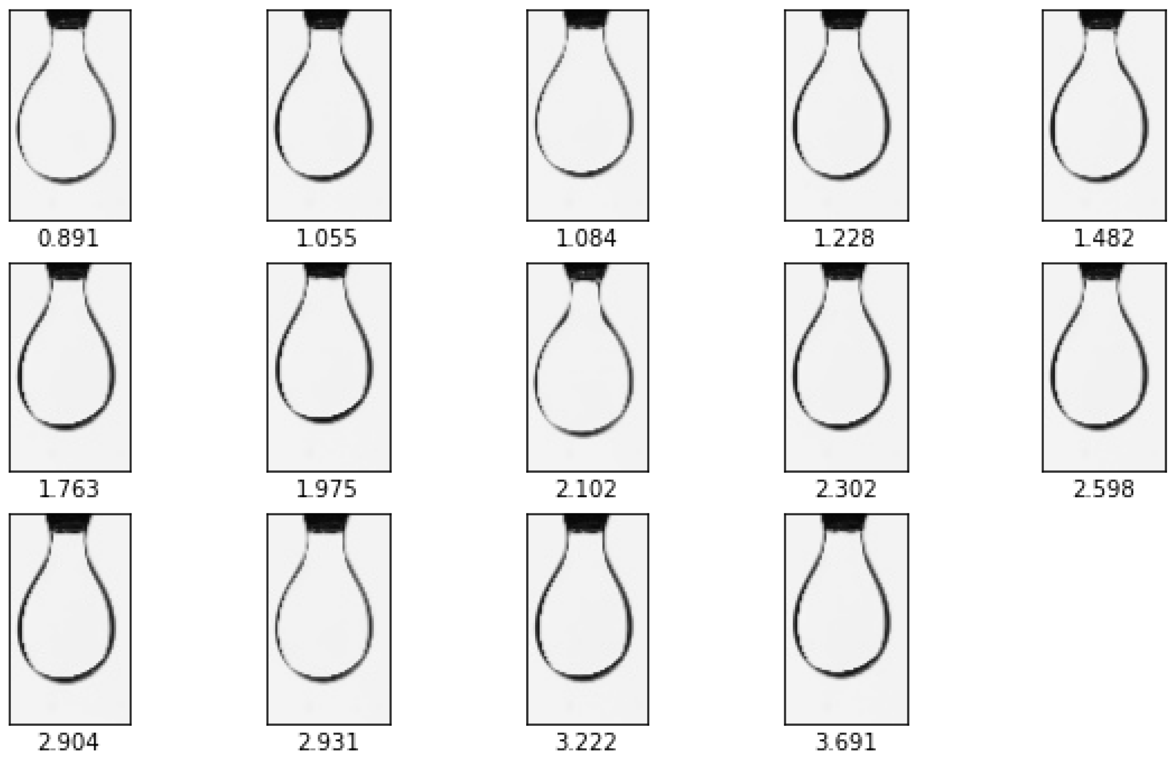
| Formulation Name (PVP%) | Viscosity in mPa·S |
|---|---|
| PVP00.0 | 0.891 |
| PVP05.0 | 1.055 |
| PVP07.5 | 1.084 |
| PVP10.0 | 1.228 |
| PVP15.0 | 1.482 |
| PVP20.0 | 1.763 |
| PVP25.0 | 1.975 |
| PVP27.5 | 2.102 |
| PVP30.0 | 2.302 |
| PVP35.0 | 2.598 |
| PVP40.0 | 2.904 |
| PVP42.5 | 2.931 |
| PVP45.0 | 3.222 |
| PVP50.0 | 3.691 |
| Formulation Name (PVP%) | Number of Images |
|---|---|
| Training and validation set | |
| PVP00.0 | 437 |
| PVP05.0 | 450 |
| PVP10.0 | 473 |
| PVP15.0 | 447 |
| PVP20.0 | 394 |
| PVP25.0 | 440 |
| PVP30.0 | 393 |
| PVP35.0 | 442 |
| PVP40.0 | 440 |
| PVP45.0 | 435 |
| PVP50.0 | 437 |
| Testing set | |
| PVP07.5 | 425 |
| PVP27.5 | 422 |
| PVP42.5 | 439 |
| Total | 6074 |
| SimpleModel | DeepModel * | ComplexModel | |
|---|---|---|---|
| Results on the training set | |||
| MSE | 0.1297 | 0.0144 | 0.0185 |
| MAE | 0.3010 | 0.0906 | 0.1092 |
| R2 | 0.8328 | 0.9813 | 0.9761 |
| Results on the validation set | |||
| MSE | 0.1530 | 0.0142 | 0.0223 |
| MAE | 0.3215 | 0.0903 | 0.1186 |
| R2 | 0.8174 | 0.9829 | 0.9733 |
| Results on the testing set | |||
| MSE | 0.1798 | 0.0243 | 0.0400 |
| MAE | 0.3633 | 0.0971 | 0.1504 |
| R2 | 0.6867 | 0.9576 | 0.9302 |
Disclaimer/Publisher’s Note: The statements, opinions and data contained in all publications are solely those of the individual author(s) and contributor(s) and not of MDPI and/or the editor(s). MDPI and/or the editor(s) disclaim responsibility for any injury to people or property resulting from any ideas, methods, instructions or products referred to in the content. |
© 2023 by the authors. Licensee MDPI, Basel, Switzerland. This article is an open access article distributed under the terms and conditions of the Creative Commons Attribution (CC BY) license (https://creativecommons.org/licenses/by/4.0/).
Share and Cite
Mrad, M.A.; Csorba, K.; Galata, D.L.; Nagy, Z.K.; Charaf, H. Droplet Based Estimation of Viscosity of Water–PVP Solutions Using Convolutional Neural Networks. Processes 2023, 11, 1917. https://doi.org/10.3390/pr11071917
Mrad MA, Csorba K, Galata DL, Nagy ZK, Charaf H. Droplet Based Estimation of Viscosity of Water–PVP Solutions Using Convolutional Neural Networks. Processes. 2023; 11(7):1917. https://doi.org/10.3390/pr11071917
Chicago/Turabian StyleMrad, Mohamed Azouz, Kristof Csorba, Dorián László Galata, Zsombor Kristóf Nagy, and Hassan Charaf. 2023. "Droplet Based Estimation of Viscosity of Water–PVP Solutions Using Convolutional Neural Networks" Processes 11, no. 7: 1917. https://doi.org/10.3390/pr11071917
APA StyleMrad, M. A., Csorba, K., Galata, D. L., Nagy, Z. K., & Charaf, H. (2023). Droplet Based Estimation of Viscosity of Water–PVP Solutions Using Convolutional Neural Networks. Processes, 11(7), 1917. https://doi.org/10.3390/pr11071917