Abstract
Hydraulic fracturing is one of the main ways to increase oil and gas production. However, with existing methods, the diameter of the nozzle cannot be easily adjusted. This therefore results in ‘sand production’ in flowback fluid, affecting the application of hydraulic fracturing. This is because it is difficult to identify the one-dimensional series signal of fracturing fluid collected on site. In order to avoid ‘sand production’ in the flowback fluid, the nozzle should be properly controlled. Aiming to address this problem, a novel augmented residual deep learning neural network (AU-RES) is proposed that can identify the characteristics of multiple one-dimensional time series signals and effectively predict the diameter of the nozzle. The AU-RES network includes three parts: signal conversion layer, residual and convolutional layer, fully connected layer (including regression layer). Firstly, a spatial conversion algorithm for multiple one-dimensional time series signals is proposed, which can transform the one-dimensional time series signals into images in high dimensional space. Secondly, the features of the images are extracted and identified by the residual network. Thirdly, the network hyperparameters are optimized to improve the prediction accuracy of the network. Simulations and experiments performed on the field data samples show that the RMSE and LOSS when training the AU-RES network are 0.131 and 0.00021, respectively, and the prediction error of the test samples is 0.1689. In the gas field experiments, fracturing fluid sand production could be controlled, thus demonstrating the validity and reliability of the AU-RES network. By using the AU-RES neural network, sand particles will not be present in the flowback of fracturing fluid, thus improving the efficiency of hydraulic fracturing and reducing the cost of hydraulic fracturing. In addition, the AU-RES network can also be used in other similar situations.
1. Introduction
Artificial intelligence has become a research hotspot, and will come to be widely used in various industries [1,2], especially in the oil and gas industry [3,4,5,6]. In the process of oil and gas recovery, hydraulic fracturing technology is widely used to increase production. In the context of hydraulic fracturing technology, flowback control of the fracturing fluid is an aspect belonging to process control, and is achieved by controlling the opening or closing of the nozzle at the wellhead according to the downhole fluid parameters. This results in the diameter of the nozzle being adjusted. In this way, no sand is produced in the fracturing fluid. However, conventional control methods are inefficient and sand particles in the formation can easily be discharged with the flowback of fracturing fluid, resulting in a ‘sand production’ problem. Therefore, the introduction of artificial intelligence technology into the flowback control process of fracturing fluid is necessary, as it will be able to solve this problem.
When considering the use of artificial intelligence in the flowback control of fracturing fluid, research has been performed evaluating a number of different methods, including fuzzy control [3], shallow artificial neural network control [7], deep artificial neural network control [8,9,10] (such as CNN, LetNet, VGG16, Alexnet), and so on. However, because the flowback control of fracturing fluid is characterized by strong nonlinearity, and some of the downhole parameters are difficult to obtain, it is necessary to use the deep learning neural network, which can achieve good results. The conventional deep neural networks, i.e., the CNN, LetNet, VGG16, Alexnet networks, are often used in image classification. Although they can output a continuous value if their last layer (the activation function Softmax) can be substituted by a regression layer, the accuracy will be low. Therefore, these neural networks should be modified to adapt their prediction of continuous values [11] such as the nozzle diameter. In essence, the fracturing fluid flowback control identifies multiple one-dimensional signals in oil and gas wells using a deep learning neural network, then performs high-level feature transformation, and outputs a continuous signal (nozzle diameter). Therefore, its structure is similar to that of the long short-term memory (LSTM) network [12,13] and certain kinds of temporal convolutional network (TCN) [14].
To date, LSTM, TCN and other similar methods have been studied by many researchers. Hu Xiaodong [7] proposed a shale gas production prediction model with a fitting function neural network. The model, consisting of a fitting function, LSTM and a DNN neural network, predicts the parameters according to time domain signals. Zhang Lei et al. [12] proposed a time-domain convolutional neural network TCN model to solve the problem of time-domain signal prediction. Sagheer A [13] proposed a kind of deep LSTM recurrent network for predicting production. BAI S J et al. [14] evaluated convolutional networks and recurrent networks for time sequence signal modeling. In addition, they proposed a combination of convolutional networks with recurrent networks. Gu Jianwei [15] introduced an LSTM network to predict oil production. Huang R J [16] used an LSTM network to forecast the production performance of a carbonate reservoir. Wang J [17] studied a hybrid network of CNN and LSTM to forecast the production of fractured wells, overcoming the shortcomings of the traditional method, which relies on personal experience. In essence, LSTM is used to predict future values according to historical data. However, for the control of the flowback of fracturing fluid (or nozzle diameter prediction), it is necessary to determine the current value (nozzle diameter) according to multiple kinds of current signal and the historical signal. Therefore, the above methods still present challenges in terms of processing these unstructured data and processing multiple one-dimensional time series signals, such as those related to the flowback of fracturing fluid. In addition, the inclusion of a CNN layer in LSTM or TCN results in degradation when the training epoch increases. Therefore, the accuracy of the LSTM or TCN network will decrease.
From the above discussion, it is clear that the neural networks described above cannot be directly applied in the flowback control of fracturing fluid, due to the complexity of the fracturing flowback process. In this case, the nozzle diameter needs to be predicted based on multiple one-dimensional time series signals. In addition, it is necessary to consider not only the dynamical factors affecting the nozzle diameter, but also the static factors affecting the nozzle diameter. Therefore, an augmented residual deep learning neural network (AU-RES) structure is proposed to control the fracturing flowback process. Firstly, the spatial transformation of multiple one-dimensional time series signals of fracturing flowback is carried out. Then, the conventional residual neural network structure [18] is modified to form a new AU-RES neural network to control the flowback of fracturing fluid. Next, the AU-RES neural network is used to identify and judge the input signal, and outputs a nozzle diameter. Finally, the performance of the AU-RES network is verified by simulation and experiment.
2. Problem Description and Solution
2.1. Problem Description
The principle of fracturing flowback control is shown in Figure 1a, and includes two steps. First step: the fracturing fluid containing sand is firstly injected underground at high pressure from the ground surface. The high-pressure fluid creates cracks in the rock. Sand particles in the fluid support cracking, so that oil or gas from the rock will permeate into the well. Second step: after a crack or fracture has been formed in the rock, the fracturing fluid needs to flow back to the surface. Fracturing fluid flows through the well via the oil tube, and then flows out through the surface nozzle. During this process, the sand needs to remain in the fracture, otherwise it will close again. In order to prevent sand in the fracture from flowing out of the well, it is necessary to control the ground nozzle. Therefore, methods for determining an optimal nozzle diameter constitute a core problem of fracturing flowback control.
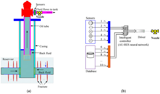
Figure 1.
Principle of hydraulic fracturing and intelligent control scheme. 1—Fluid pressure; 2—flow rate; 3—viscosity; 4—temperature; 5—sand rate; 6—pressure in reservoir; 7—permeability; 8—porosity; 9—Poisson’s ratio of rock; 10—fracture length; 11—fracture height; 12—inner diameter of oil tube; 13—inner diameter of casing; 14—depth of gas well. (a) Principle of hydraulic fracturing. (b) Intelligent control scheme.
In the past, the method for determining the diameter of the nozzle usually involved analyzing the hydrodynamic formula of flowback fluid, on the basis of which an approximate solution for the nozzle diameter was obtained. For example, in Figure 1a, when the diameter of the nozzle changes, the inlet pressure (at the left side of the nozzle) pd will also change. In addition, the fluid in the oil tube transmits the pd to the bottom well. Therefore, the pressure pr at the bottom well will also change. pd is the inlet pressure of the nozzle, which reflects the fluid pressure in the oil tube before the nozzle. pr is the formation pressure, which reflects whether the fracturing particles can leave the rock fractures (cracks). The pressure pd and pr can be written as:
In Equations (1) and (2), t is time. x1, x2, x3, …, xn parameters related to the flowback fluid in the oil tube. d is the nozzle diameter. Po is the outlet pressure of the nozzle (at the right side of the nozzle). Because φ ( ) and f ( ) are nonlinear functions and Equations (1) and (2) involve multiple hydrodynamic differential equations, it is difficult to obtain a precise solution. The prediction error of the nozzle diameter using the traditional method is large. Therefore, a problem to be solved is to predict the nozzle diameter according to the nonlinear function relationship in the variable x1~xn simulation Equations (1) and (2).
2.2. Solution
In order to solve the problem of the large error when predicting the nozzle diameter using traditional methods, a new artificial intelligence method is proposed for predicting nozzle diameter. The scheme is shown in Figure 1b. The intelligent controller in Figure 1b is the deep learning neural network. In this paper, we introduce a novel augmented residual deep learning neural network (AU-RES) that is able to identify time series signals of flowback fluid on the basis of the characteristics of fracturing flowback fluid signals, thus allowing accurate prediction of the nozzle diameter.
The principle of Figure 1b is as follows: firstly, fracturing fluid flowback parameters are collected and fed into the AU-RES neural network. Secondly, the AU-RES neural network extracts the features of the input data (x1~x14) and recognizes it according to the self-learning algorithm. Thirdly, the AU-RES neural network outputs the diameter of the nozzle. Because AU-RES neural networks can simulate the complex nonlinear functional relationships in Equations (1) and (2), when trained with field data, the neural networks can learn from the experience of the operator. Therefore the AU-RES neural network can achieve good control effect.
In Figure 1b, x1~x5 change over time. Therefore, they need to be collected with sensors. x1 is the oil pressure in the flowback fluid. x2 is the casing pressure. x3 is the flow rate. x4 is viscosity. x5 is the temperature of the flowback fluid. The signals for x6~x14 generally do not change with time. Therefore, they can be obtained from the database. x6 is the pressure of the formation. x7 is permeability. x8 is porosity. x9 is crack half-length. x10 is crack height. x11 is the Poisson’s ratio of the rock. x12 is the inner diameter of the casing. x13 is the inner diameter of the oil tube. x14 is the depth of the oil/gas well.
Focusing on the characteristics x1~x14, the AU-RES neural network was designed as shown in Figure 2. The input data for the AU-RES neural network are the time series signals, and the output is the diameter of the nozzle. The network includes a signal conversion layer, a residual connection layer, and a fully connected layer (including regression layer). The function of the signal conversion layer is to transform the one-dimensional time series signals into a two-dimensional image so that the neural network can identify it better. For the first layer, x1~x14 are time series signals, as shown in Figure 1. These signals are input into the signal conversion layer. The function of the residual connection layer is to extract the high-level features from the inputted images to identify the different time series signals. In order to distinguish the differences in time series signals, the sublayers Stem, Incept-A, Incept-B, Incept-C, and Incept-D are used, which have different convolutional nodes. The function of convolution is to extract information from the input image. The role of pooling is to perform feature selection, thereby reducing the number of features, and thus the number of parameters. In this paper, the residual connection layer is transferred directly from the Res-incept-V2 neural network, which absorbs the transfer learning neural network [19]. The fully connected layer transforms the high-level features (matrices) into large one-dimensional vectors that can identify images and output a continuous value (i.e., nozzle diameter). The regression layer must be located at the end of the AU-RES neural network. Because the AU-RES neural network outputs a continuous value, it is a regression problem, rather than a classification problem.
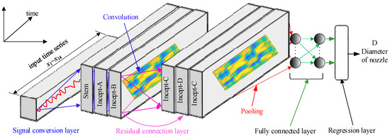
Figure 2.
Structure of AU-RES neural network.
3. Algorithm of AU-RES Neural Network
3.1. Signal Conversion in the Time Domain
The data collected in Figure 1b include x1~x14. However, in practice, these data have different effects on nozzle diameter. x1~x5 denote real-time data collected during fracturing fluid flowback. These data change frequently, and are the main factor affecting nozzle diameter, while x6~x14 are data measured off-line, and are generally stored in the database. They rarely change, and are minor factors affecting the nozzle diameter. In addition, there are other parameters, but because these parameters have very little influence on nozzle diameter, they are ignored, and their influence is implied in the weight of the AU-RES neural network. Therefore, the data transformation algorithm is designed according to the characteristics of these data.
We can define one-dimensional time series signals x1 = [x11, x12, …, x1M], x2 = [x21, x22, …, x2M], …, x5 = [x51, x52, …, x5M], where x1~x5 are shown in Figure 1b. M is the sample number. Therefore, they can be written as:
xI = [ xi1, xi2, …, xiM], i = 1~5
We can also define another one-dimensional signal, as follows:
In Equation (4), we want to extend x6~x14 in Figure 1b as vectors, so that variations in nozzle diameter can be reflected.
Definition 1.
We define a multi-variant time series and non-time series signal:
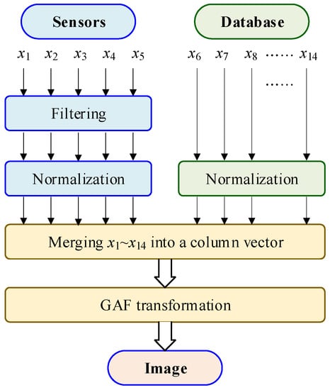
where x1~x5 are time series signals, and is a single data point, in which x1~x5 , . Therefore, X is a column vector and X , and we merge all the data in Figure 2 to X. When M = 28, the length of X is 307. Because the signals x1~x5 contain noise, we need to filter the signals, as shown in Figure 3. In Figure 3, the input signals include x1~x5 and . The process of data merging is shown in Figure 4. Since the amplitude of the input signals are inconsistent, it needs to be normalized to convert its amplitude to [0–1]. The normalization equation is:
where Xi is the ith element of X. is the normalized result. The normalized data can meet the requirement of neural network. In the next module, all the components of are combined to form a column vector with dimensions of 10M + 27. Finally, a matrix, namely a two-dimensional image, is formed by the algorithm presented as Equation (8).

Figure 3.
Algorithm of data conversion.

Figure 4.
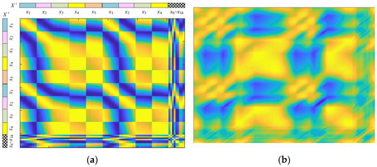
The image converted by the GAF transformation. (a) Clear image. (b) Blurred and fuzzy image.
Definition 2.
We also define a dataset:
D = {(X1,Y1), (X2,Y2), …, (XN,YN)}
D is taken as the training sample and testing sample for the AU-RES network. Y is the diameter of the nozzle, which is a continuous number. Therefore, the task of the AU-RES network is to find the map between the time series signal X and the nozzle diameter. Note that this is a regression problem, which is different from the problem of time series classification.
Next, we create a mapping relationship, X→I, which converts X into a two-dimensional matrix (image) using the following equation:
where I , which is similar to the GAF transformation [20,21,22,23].
The matrix I can be drawn as an image, as shown in Figure 4. Figure 4a is a clear image that includes many square lattices. Every lattice reflects the relationship between xi and xj. Therefore, this image can represent the characteristics of x1~x14. The blue color (dark color) represents low signal amplitude (the lowest value is 0), and the yellow color (bright color) represents high signal amplitude (the highest value is 1). Therefore, the color of the image reflects the distribution of the original signal amplitude. In order to improve the generalization ability of the neural network, it is necessary to convert clear images into fuzzy images. Therefore, Figure 4a is blurred, and the fuzzy image is shown at Figure 4b.
3.2. Residual Neural Network
In the course of our research, we compared different networks, such as Lenet, Alexnet, VGG16, residual network Inception V2, etc., and we found that the residual network [24,25,26] had the best performance, so the residual network was used to predict the nozzle diameter. The residual network was proposed by Kaiming HE [18,24], and consists of different residual modules; the basic residual module is shown in Figure 5.
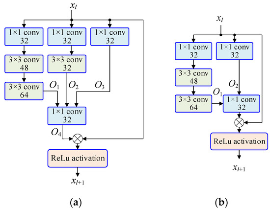
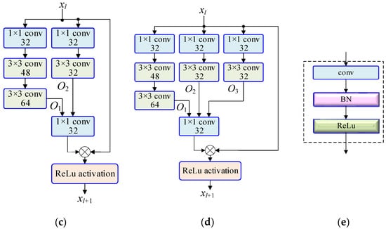
Figure 5.
The basic residual modules. (a) Incept-A. (b) Incept-B. (c) Incept-C. (d) Incept-D. (e) Inner structure of i × i conv in Incept-A~Incept_D (i = 1,3).
In Figure 5, it can be seen that the residual neural network includes 4 kinds of residual module, with each module having a different function. Different module combinations are designed in the residual network to sense different visual fields in the image, that is, to extract different features of the image. In addition, there is a phenomenon in deep learning neural networks whereby if the number of network layers is small, the training error will be large, but if the number of network layers is too large, a “degradation” phenomenon can easily occur, that is, the network accuracy will decrease instead of increasing. Therefore, a direct channel is added to the residual network, the main purpose of which is to retain the image information (after many convolutional layers have been transformed, the original information of the image may disappear, resulting in network degradation). By employing this setting, the residual network can not only obtain higher precision, but the degradation phenomenon can also be avoided.
Figure 5a shows the residual module of Incept-A, which has 4 channels to convert the input signal. From left to right, in the first channel, the image is converted through 1 × 1, 3 × 3, and 3 × 3 convolutional layers. Where ‘1 × 1 conv 32′ means the kernel size is 1 × 1, and the depth is 32. Every ‘conv’ includes a convolutional layer, a batch normalization (BN) layer and an activation function (ReLu), as is shown in Figure 5e. Similarly, in the second channel, the image is converted through 1 × 1 and 3 × 3 convolutional layers. In the third channel, the image is converted through a 1 × 1 convolutional layer. The first layer, the second layer and the third layer are all connected to a 1 × 1 convolutional layer. This layer plays the role of changing the image dimensions so that the dimensions are the same as those of the fourth channel. If the input image is 64 × 64, the output O1 is 60 × 60, the output O2 of the second channel on the left is 62 × 62, and the output O3 of the third channel on the left is 64 × 64, since the dimensions of the three images are inconsistent, it is necessary to perform a transformation in the 1 × 1 convolutional layer to obtain an output image with dimensions of 64 × 64. The fourth channel is the direct channel of the image, which reflects the ‘identity mapping’. This channel is very important for the residual neural network, and can reserve the information in the image during signal conversion. Therefore, network degradation during training can be avoided, and the precision of the network can be improved. Because of the existence of the identity mapping layer, the error of image recognition can be reduced.
In the same way, Figure 5b shows Incept-B, which consists of three channels. Figure 5c shows Incept-C, which consists of three channels. In addition, Figure 5d shows Incept-D, which consists of four channels. These modules contain different numbers of convolutional layers. Compared with Incept-A and Incept-D, the third channel on the left of Incept-A has only one convolutional layer, while the third channel on the left of Incept-D has two convolutional layers. Therefore, the output O3 of Incept-A is different from that of Incept-D.
3.3. AU-RES Neural Network
Based on the structure of the residual network, we added a data feature transformation layer and a fully connected layer to form a new AU-RES neural network. The structure of the AU-RES neural network is shown in Figure 6. Layer 1 is the signal conversion layer in Figure 2. It can convert multiple one-dimensional time series signals into a two-dimensional image. Layer 2 is the residual connection layer in Figure 2, which can extract the high-level features of the input image. In layer 2, the ‘stem’ includes 12 convolutional layers, 12 batch normalization layers, 12 activation functions (ReLu), a max-polling layer, and an average-pooling layer. Since the structure of ‘stem’ in layer 2 is the same as that of Res-Inception-V2, the detailed structure of the ‘stem’ is not drawn here. Layer 3 is the fully connected layer, and the last part is the regression layer, which outpus a value for nozzle diameter.
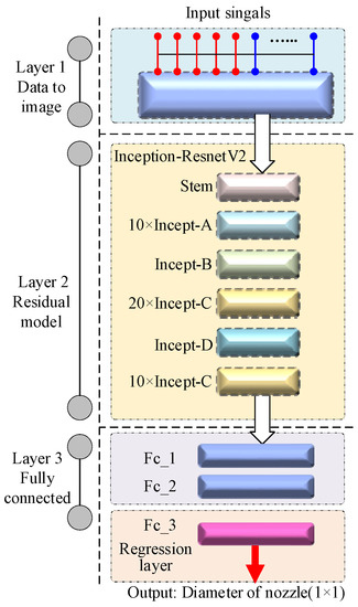
Figure 6.
Structure of AU-RES neural networks.
3.4. Loss Function
Since the AU-RES network outputs continuous values, the mean square error MSE is used as the loss function, as follows:
where is the expected output. Yt is the actual output. n is the number of training samples. Loss reflects the difference between the actual output and the expected output.
3.5. Training Algorithm
The training algorithm is shown in Figure 7, and can be described as follows:
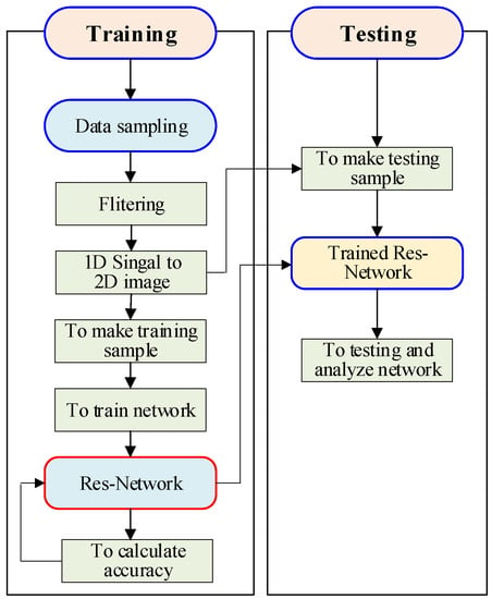
Figure 7.
Training algorithm.
- Step 1: Data are collected on site. Then, unreasonable data are filtered out and deleted. Finally, samples are made using the processed data. The input to the residual model in the AU-RES neural network is the two-dimensional image of the data transformation, including flow, pressure, and temperature. In addition, the output of the AU-RES neural network is the label (Y in Equation (6)).
- Step 2: The finite element difference method is used to calculate the downhole fluid dynamics model, supplementing the simulated sample.
- Step 3: The neural network hyperparameters and initial values are set.
- Step 4: 80% of samples are selected as the training set to train the neural network.
- Step 5: Whether the AU-RES neural network training process converges is observed.
- Step 6: 20% of the sample set is used as the test set to study the influence of different hyperparameters on the prediction accuracy and optimize the AU-RES neural network structure. Here, we introduce an index of prediction error E for AU-RES.where represents the norm of Euclidean space vectors.
- Step 7: Training process finished.
4. Simulation and Experiment
4.1. Training Sample
Training samples for the AU-RES network come in two types: samples collected on site, and simulated samples calculated using the finite element difference method. The flow rate, fluid pressure, fluid temperature, fluid viscosity, and sand content in the fluid are collected at 1 min intervals at the gas well site. When the AU-RES neural network is trained, the training sample is input to the AU-RES neural network, and the label is added to the output end of the neural network. Here, the label is nozzle diameter (Yi in Equation (6)).
These samples (one-dimensional time series signals) are transformed into images in the signal conversion layer. Images are shown in Figure 8 that correspond to nozzle diameters from 3 mm to 13 mm. In Figure 8, the blue color (dark color) represents low signal amplitude (the lowest value is 0), and the yellow color (bright color) represents high signal amplitude (the highest value is 1). Different color distributions in the image represent changes in the amplitude of the input one-dimensional time series signals. Therefore, the overall color of the image reflects the nozzle diameter corresponding to the time series signal.
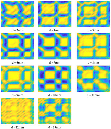
Figure 8.
Images transformed by the signal conversion layer in the AU-RES network.
4.2. Training Process
The training samples are input into the AU-RES neural network to train the AU-RES neural network. The parameters corresponding to node number and convolutional kernels in the convolutional layer and the pooling layer in the AU-RES network are the same as those of Res-Inception-V2. The initial bias value of each node in the convolutional layer is set as [0.001, 0.001, …, 0.001], the weight as [0, 0, …, 0], and the initial learning rate is 0.0001. The parameter update method for the AU-RES neural network is Adam. When training the neural network, the computer configuration was as follows: the CPU was an AMD Ryzon 3 3100, and the memory (RAM) size was 24 GB. The computer graphics card was an NVIDIA GeForce GTX 1050Ti. It took 26 h to train the AU-RES neural network. However, the testing time was only 0.20 s. Therefore, the AU-RES neural network can be used in engineering applications. The AU-RES neural network was trained for 150 epochs, and its convergence was observed, as shown in Figure 9. Figure 9a represents the training RMSE, which reflects the Root Mean Square Error between the actual output and the expected output of the training sample. Figure 9b represents the training loss, which reflects the loss function in Equation (8) between the actual output and the expected output of the training sample. When training the AU-RES neural network, loss can often be used to calculate the gradient and update the weight value of each node. As can be seen from Figure 9, after 150 epochs of training, the RMSE value converges stably to 0.131, and the loss value converges to 0.00021, which indicates that the AU-RES neural network parameters have reached their optimal values. The AU-RES neural network training process is concluded.
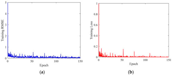
Figure 9.
AU-RES neural network training process. (a) Training RMSE. (b) Training Loss.
4.3. The Influence of Hyperparameters on AU-RES Network Performance
AU-RES neural network hyperparameters include internal node number, convolution kernel size, learning rate, and gradient update method. In this paper, since the number of nodes and the convolutional kernel of the convolutional layer are the same as those of the residual network Res-Inception-V2, these parameters are fixed. When training the AU-RES network, the change in network performance was observed when changing the learning rate, gradient update method, and the number of nodes in the fully connected layer.
After changing the learning rate of the AU-RES neural network, we observed the change in the performance of the network, with results as shown in Table 1. As can be seen from Table 1, the AU-RES neural network performance was best when the learning rate was 0.0001.

Table 1.
The effect of using different learning rates on the performance of the neural network.
The gradient update method is changed, with Sgdm, Adam and RMSprop being employed, respectively. The test error of the different methods after network training was observed, with results as shown in Table 2. It can be seen that when the Adam method was adopted, the test sample prediction error E was the lowest, which means that the accuracy of the network was the highest.

Table 2.
The effect of update method of hyperparameters on the performance of the neural network.
4.4. The Influence of the Fully Connected Layer on AU-RES Network Performance
The number of nodes in the fully connected layer can be changed, and the corresponding changes in AU-RES network performance can be observed, as shown in Figure 10. The fully connected layer of the AU-RES network is divided into three layers, among which the number of nodes in the third layer must be consistent with the dimensions of the output signal. Since the output of the AU-RES network is a one-dimensional continuous value, the number of nodes in the third layer (i.e., the regression layer) network can only be 1. However, we can change the number of nodes in layer 1 and layer 2 to find the best fully connected layer structure. Here, the number of nodes is adjusted from 16 to 64. If the number of nodes is too great, the computing speed will decrease, and overfitting will occur. As can be seen from Figure 10, the RMSE reaches its lowest value of 0.1605 when fc1 = 24 and fc2 = 32. Therefore, the performance of the AU-RES neural network is the best.
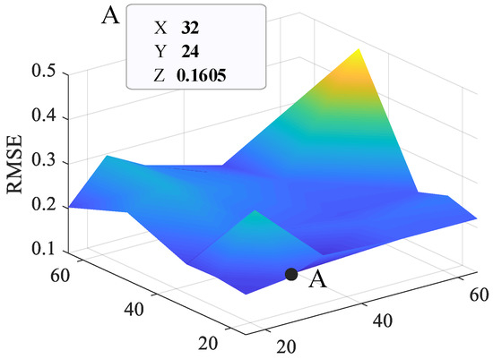
Figure 10.
The effect of the number of fully connected layer in the performance of neural network.
4.5. Comparison of AU-RES Network with Other Networks
The AU-RES neural network was compared with other deep learning neural networks, and the simulation results are shown in Figure 11. In the past, the experience control method has often been used for fracturing flowback control, but there were no artificial intelligence methods available. Therefore, there are no articles comparing their results. In this paper, we only compared the results of the AU-RES neural network with those of other deep learning neural networks. The selected deep learning neural networks include LetNet5, AlexNet, VGG16, etc. When training the networks, the learning rate of the networks was 0.0001, and the hyperparameter update method was Adam. The number of epochs for neural network training was 150. Then, the same test sample was input into different neural networks, and the output of each neural network was observed, as shown in Figure 11 and Table 3. As these deep learning neural networks are often used for image recognition, the RegressionLayer for the final layer needs to be changed to ClassficationLayer, so that the networks can output continuous values.
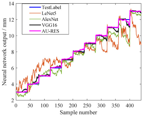
Figure 11.
Comparison of the AU-RES network with other networks.

Table 3.
Performance of the different neural networks.
In Figure 11, the blue line ‘TestLabel’ is the output label of the neural network, which is equivalent to the expected output of the neural network. The orange line ‘LeNet5′ represents the actual output of LeNet5 neural network. The green line ‘AlexNet’ represents the actual output of the AlexNet neural network, the black line ‘VGG16′ represents the actual output of the VGG16 neural network, and the purple line ‘AU-RES’ represents the actual output of the AU-RES neural network proposed in this paper. The values of these curves range from 3 to 13. If a curve is far from the blue line, it has a large error. As can be seen from Figure 11, the LeNet5 network exhibited the largest error. The reason for this is that the network has a simple structure and can only recognize the characters 0–9, so it has difficulty recognizing complex continuous one-dimensional time series signals. AlexNet is a mature transfer learning neural network with increased network depth, so its recognition accuracy is higher than LeNet5 network. VGG16 is a deeper neural network, so its recognition accuracy is further improved. The AU-RES network studied in this paper is an augmented residual neural network. Because the data transformation layer is added and the residual layer and the fully connected layer are improved, the prediction accuracy is the highest. The total error of the output signal of the AU-RES neural network is 0.1689, which indicates the superiority of the AU-RES neural network.
4.6. Experiment
On the basis of the AU-RES neural network algorithm studied in this paper, control software was developed. We installed the software on an intelligent controller, so as to produce a prototype of the intelligent control device for fracturing fluid flowback. The prototype of the intelligent control device is shown in Figure 12.
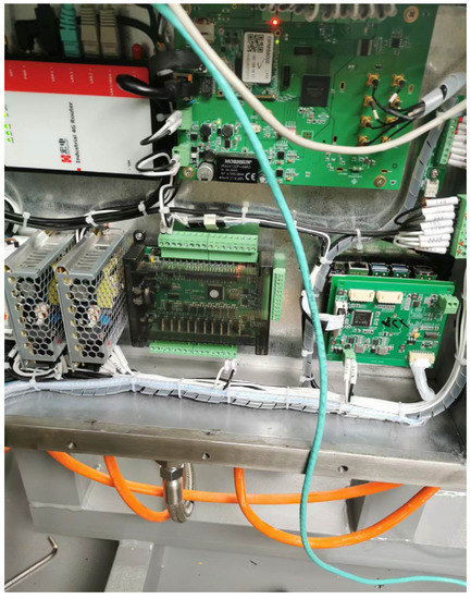
Figure 12.
Intelligent controller prototype for fracturing fluid flowback.
The prototype was applied to a gas field experiment. During the experiment, the main parameters of the fracturing fluid in the oil tube were collected once an hour, and the results are shown in Table 4. In Table 4, the data in the first column represent time, and the data in the second to fourth columns correspond to the main fracturing fluid parameters in the oil tube, and the data in the seventh column indicate the nozzle diameter predicted by the AU-RES neural network. Through the experiment, it was found that there was no sand present in the fracturing fluid, indicating that the AU-RES neural network was able to correctly predict the diameter of the nozzle, and the experiment was successful.

Table 4.
The main data collected during the experiment.
When training the AU-RES neural network, it is necessary to collect a lot of data from the oil and gas field. This is a potential limitation or challenges for the application of the AU-RES neural network. Sometimes, these data are difficult to obtain due to data privacy. However, the AU-RES neural network is often used in industrial enterprises. Because they have a lot of data, they are able to easily train the AU-RES neural network.
5. Conclusions
Through the research of this paper, the following conclusions can be drawn:
In the process of hydraulic fracturing flowback control, it is difficult for traditional methods to achieve good results due to a variety of nonlinear and uncertain factors, leading to the problem of ‘sand production’. An artificial intelligence method consisting of the AU-RES neural network can solve this problem well, and the field experiment results were good.
The AU-RES neural network was based on an existing residual network, adding a signal conversion layer to transform one-dimensional time series signals into two-dimensional images that can better adapt to the characteristics of the residual network, thus improving the prediction accuracy.
In the AU-RES neural network, the performance of the neural network can be improved by optimizing the hyperparameters (learning rate, gradient update method, number of nodes in the fully connected layer, etc.) After optimization, the learning rate was 0.0001. The gradient update method used was ‘Adam’. The fully connected layer had 3 sublayers, i.e., Fc_1, Fc_2 and Fc_3, among which Fc_1 had 24 nodes and had Fc_2 32 nodes. The RMSE and loss of AU-RES network training were 0.131 and 0.00021, respectively, and the prediction error of the test samples was 0.1689.
The AU-RES neural network can effectively predict multiple one-dimensional time series signals and explore their signal features. It can be applied not only to tight gas fracturing fluid flowback control, but also to other industries, where one-dimensional timing signals need to be identified and predicted. Therefore, this study provides a theoretical basis for the application of artificial intelligence technology in various industries.
With the development of new materials and new processes, hydraulic fracturing flowback technology has developed rapidly. The use of new nanomaterials, new proppants, new hydraulic fracturing flowback design models, and artificial intelligence to control the flowback process have greatly improved the efficiency and quality of hydraulic fracturing flowback.
Author Contributions
Conceptualization, H.W.; writing—original draft preparation, R.L.; software, J.W.; funding acquisition, B.L.; formal analysis, X.Z.; data curation, W.B. All authors have read and agreed to the published version of the manuscript.
Funding
This research was funded by the Natural Science Basic Research Program of Shaanxi, grant number 2021JM-405, Xi’an Science and Technology Plan, grant number 22GXFW0103, and supported by the Postgraduate Innovation and Practice Ability Development Fund of Xi’an Shiyou University, grant number YCS23114171.
Acknowledgments
Oil and gas field companies provided field data for this article. The authors express their gratitude to them.
Conflicts of Interest
The authors of this article declare that there are no known competing financial interest or personal relationship that could influence the work presented in this article.
References
- Aloysius, N.; Geetha, M. A review on deep convolutional neural networks. In Proceedings of the 2017 IEEE International Conference on Communication and Signal Processing, ICCSP 2017, Chennai, Tamilnadu, India, 6–8 April 2017; pp. 588–592. [Google Scholar]
- Sharma, N.; Jain, V.; Mishra, A. An analysis of convolutional neural networks for image classification. Procedia Comput. Sci. 2018, 132, 377–384. [Google Scholar] [CrossRef]
- Lin, B.; Guo, J. Discussion on current application of artificial intelligence in petroleum industry. Pet. Sci. Bull. 2019, 4, 403–413. [Google Scholar] [CrossRef]
- Zhang, S.; Chen, Z. Status and prospect of artificial intelligence application in fracturing technology. Pet. Drill. Tech. 2023, 51, 69–77. [Google Scholar]
- Hui, G.; Chen, S.; He, Y.; Wang, H.; Gu, F. Machine learning-based production forecast for shale gas in unconventional reservoirs via integration of geological and operational factors. J. Nat. Gas Sci. Eng. 2021, 94, 104045. [Google Scholar] [CrossRef]
- Liu, W.; Liu, W.D.; Gu, J.W. Forecasting oil production using ensemble empirical model decomposition based Long Short-Term Memory neural network. J. Pet. Sci. Eng. 2020, 189, 107013. [Google Scholar] [CrossRef]
- Hu, X.; Tu, Z.; Luo, Y.; Zhou, F.; Li, Y.; Liu, J.; Yi, P. Shale gas well productivity prediction model with fitted function-neural network cooperation. Pet. Sci. Bull. 2022, 3, 94–405. [Google Scholar] [CrossRef]
- Zhou, L.; Yu, W. Improved Convolutional Neural Image Recognition Algorithm based on LeNet-5. J. Comput. Netw. Commun. 2022, 2022, 2022. [Google Scholar] [CrossRef]
- Su, J.; Wang, H. Fine-Tuning and Efficient VGG16 Transfer Learning Fault Diagnosis Method for Rolling Bearing. Mech. Mach. Sci. 2023, 117, 453–461. [Google Scholar]
- Zhang, C.; Zhang, H.; Tian, F.; Zhou, Y.; Zhao, S.; Du, X. Research on sheep face recognition algorithm based on improved AlexNet model. Neural Comput. Applic. 2023, 35, 1–10. [Google Scholar] [CrossRef]
- Fawaz, H.I.; Lucas, B.; Forestier, G.; Pelletier, C.; Schmidt, D.F.; Weber, J.; Webb, G.I.; Idoumghar, L.; Muller, P.-A.; Petitjean, F. InceptionTime: Finding AlexNet for time series classification. Data Min. Knowl. Discov. 2020, 34, 1936–1962. [Google Scholar] [CrossRef]
- Zhang, L.; Dou, H.; Wang, T.; Wang, H.; Peng, Y.; Zhang, J.; Liu, Z.; Mi, L.; Jiang, L. A production prediction method of single well in water flooding oilfield based on integrated temporal convolutional network model. Pet. Explor. Dev. 2022, 49, 996–1004. [Google Scholar] [CrossRef]
- Sagheer, A.; Kotb, M. Time series forecasting of petroleum production using deep LSTM recurrent networks. Neurocomputing 2019, 323, 203–213. [Google Scholar] [CrossRef]
- Bai, S.; Kolter, J.Z.; Koltun, V. An empirical evaluation of generic convolutional and recurrent networks for sequence modeling. arXiv 2018, arXiv:1803.01271. [Google Scholar]
- Gu, J.W.; Zhou, M.; Li, Z.T.; Jia, X.; Liang, Y. A data mining-based method for oil well production prediction with long and short-term memory network model. Spec. Oil Gas Reserv. 2019, 26, 77–81+131. [Google Scholar]
- Huang, R.; Wei, C.; Wang, B.; Yang, J.; Xu, X.; Wu, S.; Huang, S. Well performance prediction based on Long Short-Term Memory (LSTM) neural network. J. Pet. Sci. Eng. 2022, 208, 109686. [Google Scholar] [CrossRef]
- Wang, J.; Qiang, X.; Ren, Z.; Wang, H.; Wang, Y.; Wang, S. Time-Series Well Performance Prediction Based on Convolutional and Long Short-Term Memory Neural Network Model. Energies 2023, 16, 499. [Google Scholar] [CrossRef]
- He, K.; Zhang, X.; Ren, S.; Sun, J. Deep Residual Learning for Image Recognition. In Proceedings of the IEEE Computer Society Conference on Computer Vision and Pattern Recognition, Las Vegas, NV, USA, 27–30 June 2016. [Google Scholar]
- Alom, M.Z.; Taha, T.M.; Yakopcic, C.; Westberg, S.; Sidike, P.; Nasrin, M.S.; Van Esesn, B.C.; Awwal, A.A.S.; Asari, V.K. The history began from alexnet: A comprehensive survey on deep learning approaches. arXiv 2018, arXiv:1803.01164. [Google Scholar]
- Lyu, C.; Huo, Z.; Cheng, X.; Jiang, J.; Alimasi, A.; Liu, H. Distributed Optical Fiber Sensing Intrusion Pattern Recognition Based on GAF and CNN. J. Light. Technol. 2020, 38, 4174–4182. [Google Scholar] [CrossRef]
- Wang, Z.; Oates, T. Encoding time series as images for visual inspection and classification using tiled convolutional neural networks. In Proceedings of the 29th AAAI Conference on Artificial Intelligence, Austin, Texas, USA, 25–30 January 2015; AI Access Foundation: El Segundo, CA, USA, 2015. [Google Scholar]
- Yang, C.L.; Chen, Z.X.; Yang, C.Y. Sensor classification using convolutional neural network by encoding multivariate time series as two-dimensional colored images. Sensors 2020, 20, 168. [Google Scholar] [CrossRef]
- Gu, Y.; Wu, K.; Li, C. Rolling bearing fault diagnosis based on Gram angle field and transfer deep residual neural network. J. Vib. Shock 2022, 41, 228–237. [Google Scholar]
- He, K.; Zhang, X.; Ren, S.; Sun, J. Identity mappings in deep residual networks. In Proceedings of the 21st ACM Conference on Computer and Communications Security, Scottsdale, AZ, USA, 3–7 November 2014. [Google Scholar]
- Veit, A.; Wilber, M.J.; Belongie, S. Residual networks behave like ensembles of relatively shallow networks. Adv. Neural Inf. Process. Syst. 2016, 550–558. [Google Scholar] [CrossRef]
- Yuan, D.-R.; Zhang, Y.; Tang, Y.-J.; Li, B.-Y.; Xie, B.-L. Multiscale Residual Attention Network and Its Facial Expression Recognition Algorithm. J. Chin. Comput. Syst. 2022, 11, 1–9. [Google Scholar]
Disclaimer/Publisher’s Note: The statements, opinions and data contained in all publications are solely those of the individual author(s) and contributor(s) and not of MDPI and/or the editor(s). MDPI and/or the editor(s) disclaim responsibility for any injury to people or property resulting from any ideas, methods, instructions or products referred to in the content. |
© 2023 by the authors. Licensee MDPI, Basel, Switzerland. This article is an open access article distributed under the terms and conditions of the Creative Commons Attribution (CC BY) license (https://creativecommons.org/licenses/by/4.0/).