Recycling Strategies in a Collector-Led Remanufacturing Supply Chain under Blockchain and Uncertain Demand

Abstract

Remanufacturing has been regarded as a key to the sustainable development of enterprises. However, collection strategies affect the remanufacturing and recycling of used products. Blockchain can ensure the authenticity of disclosed information and improve the consumer’s trust in remanufactured products. Inspired by this, this paper develops a game-theoretic model to examine the selection of different recycling strategies in the remanufacturing supply chain considering blockchain adoption and uncertain demand. Incumbent collector 1 provides the manufacturer with used product 1 for remanufacturing product 1. For product 2, the manufacturer has two different collection strategies: in-house collection by the manufacturer or external collection by collector 2. The collectors act as the channel leader, and the manufacturer, who has private demand information, is the follower. Results show that collectors are incentivized to participate in the blockchain. If there is no blockchain, collector 1 prefers external collection. In the case of blockchain, the manufacturer prefers external collection when the demand variance is low. The manufacturer’s decision on the in-house collection and external collection depends on the coefficient of collection investment costs.

1. Introduction

With the development of society, environmental deterioration and resource shortages are becoming more and more serious. As an effective way to protect the environment and save resources, remanufacturing has been recognized by enterprises [1,2]. Remanufacturing is a process in which used or underperforming products are collected through recycling channels and then remanufactured. Product recycling is an essential part of remanufacturing. Different recycling modes affect optimal decision-making and pricing in a remanufacturing supply chain. In practice, a manufacturer can collect used products in three main ways. One is that the manufacturer has in-house collection channels, such as Xerox and Fuji Films [3,4]. Another is that the manufacturer assigns product collection to its retailer, such as Kodak [4]. The third one is that the manufacturer outsources the collection activity to a dedicated collector. In the literature on collection mode selection, the manufacturer is usually the leader in the supply chain, while some powerful collectors have become upstream leaders of the manufacturers in recent years, for example, IBM’s Global Asset Recovery Services, the world’s largest mobile phone recycler ReCellular, and the world’s largest metal electronics recycler SIMS Metal Management [5]. Therefore, we consider the situation that a third party performs the dedicated collection in which the collector is the leader and the manufacturer is the follower in this study.

In contrast to new products, however, consumers still have doubts about remanufactured products, such as uncertainty about the product’s quality, low evaluations, or distrust [6,7,8,9], which decreases their willingness to purchase remanufactured products. In addition, the problem of uncertain demand in the remanufacturing supply chain has also attracted considerable theoretical and practical attention. In reality, upstream collectors are unable to obtain accurate market demand information because they are not familiar with the consumer market. Market information will have a certain impact on the operational efficiency of upstream companies [10]. Accurate market demand information can help upstream collectors adjust their inventories [11] and determine the transfer price of used products [5].

Blockchain adoption can help enable the information sharing of demand and increase consumer trust in remanufactured products. Blockchain technology ensures that the information recorded in a supply chain is transparent and unalterable for all stakeholders [12], which has been widely used in information traceability. In order to reduce consumers’ concerns about quality issues, some second-hand trading platforms use blockchain technology to provide quality inspection information, such as Paipai, a second-hand trading platform of JD.com [1]. When blockchain exists, the downstream manufacturer records the demand information in the blockchain, and the upstream collector obtains full demand information. Moreover, the authenticity of disclosed information can improve consumer trust in remanufactured products. Hence, it naturally generates the following research problems:

(1)

Does the manufacturer have the incentive to participate and record the demand information in blockchain?

(2)

What are the effects of different blockchain scenarios on recycling decisions?

(3)

How do demand variance and collection investment costs affect optimal decision-making in a collector-led remanufacturing supply chain?

To solve the above problems, we consider a collector-led remanufacturing supply chain comprised of a manufacturer and two collectors. The incumbent collector 1 recycles the used product 1 and sells them to the manufacturer. The manufacturer produces two new products with raw and used materials and sells them to the market. For product 2, the manufacturer has two different recycling strategies: in-house collection (Scenario A) or external collection (Scenario B). In-house collection denotes the manufacturer recycles the used product 2, and external collection denotes collector 2 recycles the used product 2. Because of familiarity with the market, the manufacturer has full knowledge of demand information, while collectors have to make predictions about market demand. In addition, the supply chain decides whether to adopt blockchain. In the case of blockchain, the manufacturer records the demand information in blockchain, and collectors can obtain full of market demand. As a result, four models are established depending on whether the supply chain adopts blockchain or not and whether product 2’s collection is through in-house collection or through external collection (Model AN, Model BN, Model AB, and Model BB).

The main findings of this study are as follows. First, the unit transfer prices decrease with the increase in the collection rate in the four models. In Scenario B, the manufacturer’s expected profits increase in the two collection rates when in-house collection exists. In other cases, the impact of collection rates on supply chain members’ expected profits is related to the coefficient of collection investment costs. Second, the unit transfer prices and the selling quantities of product 1 in Scenario B are higher than that in Scenario A. Moreover, the unit transfer prices and selling quantities with blockchain are higher than without blockchain. However, the selling quantities of product 2 in Scenario B are lower than in Scenario A. Collectors prefer blockchain, but collector 1 is always inclined to the external collection under no blockchain. In the case of blockchain, collector 1’s decision on the external collection depends on the demand variance and the coefficient of variance. Finally, the manufacturer’s decision on the in-house collection and external collection depends on the coefficient of collection investment costs. The manufacturer may choose to implement the blockchain when the demand variance is less than a certain value.

The motivation for this research stems from the growing amount of empirical literature showing that consumers distrust the quality of remanufactured products [13,14]. Blockchain technology is an effective measure to increase consumer trust in the quality of remanufactured products. Moreover, recycling used products is a necessary link in the remanufacturing supply chain. Different recycling modes affect optimal decision-making and pricing in a remanufacturing supply chain. However, there is still a big research gap in the study of recycling models in collector-led remanufacturing supply chains, especially when considering the uncertain demand. Our findings provide new insights into blockchain applications and recycling strategies in the field of remanufacturing supply chains under uncertain demand.

The rest of this paper is organized as follows. In the next section, we briefly review the related literature. Problem formulation is listed in Section 3. Section 4 presents the collector-led supply chain models and equilibrium outcomes, respectively. In Section 5, we determine the supply chain members’ preferences for collection scenarios and blockchain adoption by comparing four models. Section 6 summarizes and concludes this study.

2. Literature Review

This research is mainly related to studies about blockchain adoption in supply chains, demand uncertainty in supply chains, and remanufacturing collection modes.

2.1. Blockchain Adoption in Supply Chains

Blockchain technology has attracted considerable attention in supply chains. Considering the manufacturer’s brand advantages and patent license fees, Yang et al. [1] studied the impact of blockchain on remanufacturing modes. Gong et al. [15] investigated the optimal strategies of the OEM regarding adopting blockchain technology and selecting distribution channels. Niu et al. [16] examined the supply chain members’ preferences for blockchain adoption considering consumers’ risk-aversion and quality distrust. Zhang et al. [17] analyzed the impact of three different blockchain adoption scenarios on the direct and retail channels of a dual-channel supply chain, where the three scenarios include both manufacturers and e-retailers adopting blockchain, manufacturers adopting blockchain, and e-retailers adopting blockchain. Cui et al. [18] used game theory to provide a theoretical investigation into the value and design of a traceability-driven blockchain under serial supply chains and parallel supply chains. Zheng et al. [19] studied the optimal blockchain-based traceability strategies in agricultural product supply chains under different strategic choices among multiple agents. Wang et al. [20] explored a three-echelon supply chain participants’ motivation, condition, and roles by analyzing the game equilibrium of the no, upper-stream, lower-stream, and entire blockchain-driven accounts receivable chains. Zhang et al. [17] explored supply chain members’ attitude towards three blockchain adoption scenarios (only manufacturer, only e-retailer, and both players) considering the direct sales channel and the retail channel. In contrast, our study focuses on the application of blockchain technology in collector-led remanufacturing supply chains. At the same time, we study the effect of blockchain adoption on the manufacturer’s different collection scenarios considering uncertain demand.

2.2. Demand Uncertainty in Supply Chains

Most studies focus on the incentives for uncertain demand exchange among supply chain members. Uncertain demand can be categorized into two types: stochastic nature and fuzzy uncertainty. Currently, most studies with uncertain needs are stochastic nature. Cai et al. [5] examined how the manufacturer shares demand information and the effects of different demand-sharing strategies on collector-led CLSCs. Huang et al. [21] developed a win-win contract based on a revenue sharing and price markdown and studied how vendors and retailers share their risks and benefits under stochastic demand during the pandemic. Ji and Liu [22] studied how the two-part tariff and ZRS contract (zero wholesale price-revenue-sharing-plus-side-payment contract) affect risks and supply chain coordination when market demand and supplier yield are both uncertain. Zhang et al. examined partial demand information sharing from three sharing methods (neither, one, or both of the manufacturers) in a supply chain consisting of a single retailer and two competitive manufacturers. Garai and Paul [23] explored supply chain coordination in a closed-loop supply chain comprising one retailer, one main supplier whose demand is stochastic uncertain, and a backup supplier. Li et al. [24] built a two-stage stochastic program and investigated a comprehensive production planning problem considering uncertain demand and risk-averse. Some other literature has studied demand uncertainty in supply chains from the perspective of fuzzy uncertainty. For example, Pei et al. [25] investigated the pricing problem of dual-channel green supply chains based on fuzzy demand. Liu et al. [26] studied the closed-loop supply chain of second-hand products with ambiguous demand and different quality levels from the perspective of centralized and different authority structures. In this paper, we also set the demand as uncertain in stochastic nature. Differently, we examine asymmetric demand information in collector-led remanufacturing supply chains. Furthermore, this paper considers blockchain adoption and compares two collection modes that have been addressed in few previous studies.

2.3. Remanufacturing Collection Modes

The third related literature stream is about how manufacturers choose collection modes for remanufacturing. For example, Zheng et al. [27] investigated how the manufacturer and retailer choose the recycling cooperation modes between recycling alliance and cost-sharing and discovered that the optimal recycling cooperation option depends on the remanufacturing efficiency and the relative recycling cost efficiency. Considering the heterogeneity of willingness to pay, Long et al. [28] explored the optimal recycling and remanufacturing decisions by comparing four different remanufacturing modes. Yi et al. [29] examined the optimal decisions on a dual recycling channel in which the retailer and the third-party collector simultaneously collect the used products in the construction machinery industry. Huang et al. [30] further studied the optimal strategies for a triple recycling channel in a retailer-dominated closed-loop supply chain. Considering the retailer’s bank loans or trade-credit financing, Zhang and Zhang [31] analyzed optimal equilibrium strategies of electric vehicle batteries in a closed-loop supply chain with a manufacturer or capital-constrained retailer recycling. He et al. [32] examined the competitive collection and channel convenience considering a manufacturer competing with a third-party collector. In the case of channel inconvenience, Guo et al. [33] investigated the optimal emission reduction strategy in three models with different recycling structures—manufacturer-led, retailer-led, and competitive under cap-and-trade regulation. Wan [34] investigated six game theory models which consist of different sales modes and recycling modes to explore the optimal pricing and recycling rate decisions under the discount coefficient of demand and the competing intensity of recycling. Some existing literature studies the collection strategies from different authority structures. For example, Cao and Ji [35] discussed the optimal recycling strategy by establishing three different Stackelberg leadership models in garment enterprises. Unlike previous literature, we investigate the optimal collection modes in a collector-led remanufacturing supply chain under demand uncertainty. Furthermore, this study also explores the impact of blockchain adoption on collection decisions.

3. Model

3.1. Problem Formulation

In our research, we consider a collector-led remanufacturing supply chain comprised of a manufacturer and two collectors. The manufacturer produces new products $i (i=1,2)$ with raw and used materials and sells them to the market at a unit retail price $p_i$. Collector $i$ recycles the used product $i$ and sells the used product $i$ to the manufacturer at a transfer price $b_i$. For product 2, the manufacturer has two different recycling strategies: in-house collection through the manufacturer (Scenario A) or external collection through collector 2 (Scenario B). We use A and B to denote the in-house collection and external collection, respectively. Motivated by Cai et al. [5], we built the supply chain structure as illustrated in Figure 1. For simplicity, we assume the manufacturer (Scenario A) and collector 2 have the same collection rate. Collectors will invest in the collection channel at a cost of $k{\lambda }_i^2$, which quadratic form of the cost function is common in previous literature. $k>0$ represents the coefficient of investment costs and ${\lambda }_i>0$ denotes the collection rate of the collector $i$. The manufacturer has a less professional recycling network channel than collector 2, so the manufacturer’s investment cost is $\varphi k{\lambda }_2^2$ in Scenario A, where $\varphi >1$ represents the proportion of collector 2’s investment costs. The unit production cost of producing a new product with raw/used materials are $c_m$, $c_r$, respectively, where $c_r<c_m$ represents the unit production cost with used materials is less than with raw materials. Denote $\Delta =c_m-c_r$, where $\Delta >b_i$ guarantees the manufacturer’s positive profit from used products.

Considering the uncertain market demand, the manufacturer has full knowledge of demand information since the manufacturer is closer to the market, while collectors have to predict the market demand. Consumers will have many uncertain concerns (including product function and product life) about remanufactured products when they know enterprises have collection channels. If blockchain is adopted, consumers can learn about the authenticity of remanufactured products and access the key information on remanufactured products from the blockchain database via cell phones. Moreover, blockchain technology can make sure the disclosed information is correct and improve the consumer’s trust in remanufactured products, which will expand the consumer market. In addition, the manufacturer will log the sales information into the blockchain. Thus, the upstream collectors can obtain accurate demand information by accessing the blockchain platform. Note that blockchain adoption is a joint decision with the manufacturer and collectors, and this study does not consider the sunk costs associated with adopting blockchain technology [36,37]. Furthermore, we do not consider the unit collection cost and only consider the investment cost of collection channel [3,5,38].

Following Niu et al. [37] and Yang et al. [38], we introduce the inverse demand function given as:

$$p_i=a_j-q_i-\beta q_{3-i}+{\epsilon }_i$$

(1)

where $j=\{B,N\}$ denotes the scenarios with/without blockchain technology and $i=\{1,2\}$ denotes the product $i$. $a_j$ stands for the deterministic market potential, where $a_B>a_N$ represents that the consumer market is expanded when blockchain exists. The random variable ${\epsilon }_i$ represents market demand uncertainty, which has a mean of zero and variance $Var[{\epsilon }_1]=rV$, $Var[{\epsilon }_2]=V$ where $0<r<1$ represents product 1 has a smaller demand variance than product 2. $\beta \in (0,1)$ represents the competition coefficient between the two products. For simplification, we assume ${\lambda }_1>{\lambda }_2>2\beta {\lambda }_1/(1+{\beta }^2)$, which represents collector 2’s collection rate is temperate. Four models are established depending on whether the supply chain adopts blockchain or not and whether product 2’s collection is through in-house collection or external collection (Model AN, Model BN, Model AB, and Model BB). We characterize supply chain members’ profits as ${\pi }_h^l$, where the subscript $h\in \{R1,R2,M\}$ stands for Collector 1, Collector 2, and the manufacturer, and the superscript $l\in \{AN,AB,BN,BB\}$ stands for the above four models.

Table 1. Notations.

Notation	Definition
$c_m/c_r$	Unit production cost of producing a new product with raw/used materials
$\Delta$	Unit saving cost of remanufacturing, $\Delta >b_i$
$\beta$	The competition coefficient between the two products
$k$	The coefficient of collection investment costs
${\epsilon }_i$	Random part of market potential for product $i$, $i$ = 1, 2
$rV/V$	The variance of the random variable ${\epsilon }_1/{\epsilon }_2$
$a_N/a_B$	The deterministic market potential without/with blockchain
${\lambda }_i$	The collection rate of product $i$, $i$ = 1, 2
$p_i$	Retail price of the product $i$, $i$ = 1, 2
${\pi }_M,\hspace{0.33em} {\pi }_{R1},{\pi }_{R2}$	The profit functions of supply chain members
Decision Variables
$q_i$	Selling quantity of the product $i$, $i$ = 1, 2
$b_i$	Unit transfer price of used product 𝑖 decided by collector $i$, $i$ = 1, 2

shows the notations in this paper.

The sequence of events is illustrated as follows. In stage 1, supply chain members decide whether to adopt blockchain technology. In stage 2, collectors decide the transfer price based on the demand information. In stage 3, the manufacturer determines the order quantities based on the transfer prices. Finally, the market demand will be realized.

3.2. Collector-Led Supply Chain Models

In this section, we investigate the four models (Model AN, Model BN, Model AB, and Model BB) and obtain the equilibrium outcomes through backward induction. To avoid trivial discussion and ensure that the equilibrium solutions are positive, we assume $(a_N-c_m)(1-\beta )>\Delta \beta {\lambda }_2$. The equilibrium outcomes are summarized in

Table 2. Outcomes in Model AN.

Model AN (i = 1, 2)
$b_1^{AN}=\left(\left(1-\beta \right)\left(a_N-c_m\right)+\Delta \left({\lambda }_1-\beta {\lambda }_2\right)\right)/2{\lambda }_1$
$q_1^{AN}=\left(\left(1-\beta \right)\left(a_N-c_m\right)+2\left({\epsilon }_1-\beta {\epsilon }_2\right)+\Delta \left({\lambda }_1-\beta {\lambda }_2\right)\right)/4\left(1-{\beta }^2\right)$
$q_2^{AN}=\left(\left(1-\beta \right)\left(\beta +2\right)\left(a_N-c_m\right)+2\left({\epsilon }_2-\beta {\epsilon }_1\right)-\Delta \left({\beta }^2{\lambda }_2+\beta {\lambda }_1-2{\lambda }_2\right)\right)/4\left(1-{\beta }^2\right)$
$E\left[{\pi }_{R1}^{AN}\right]=\left({\left(\left(1-\beta \right)\left(a_N-c_m\right)+\Delta \left({\lambda }_1-\beta {\lambda }_2\right)\right)}^2-8\left(1-{\beta }^2\right)k{\lambda }_1^2\right)/8\left(1-{\beta }^2\right)$
$E\left[{\pi }_M^{AN}\right]=\left((1-\beta )(a_N-c_m)\left((5+3\beta )(a_N-c_m)+2\Delta ({\lambda }_1+(4+3\beta ){\lambda }_2)\right)+4(1+r)V+F_1\right)/16(1-{\beta }^2)-\varphi k{\lambda }_2^2$ $F_1={\Delta }^2\left(({\lambda }_1-3\beta {\lambda }_2)({\lambda }_1+\beta {\lambda }_2)+4{\lambda }_2^2\right)$

,

Table 3. Outcomes in Model BN.

Model BN (i = 1, 2)
$b_1^{BN}=\left(\left(1-\beta \right)\left(2+\beta \right)\left(a_N-c_m\right)-\Delta \left({\beta }^2{\lambda }_1+\beta {\lambda }_2-2{\lambda }_1\right)\right)/(4-{\beta }^2){\lambda }_1$
$b_2^{BN}=\left(\left(1-\beta \right)\left(2+\beta \right)\left(a_N-c_m\right)-\Delta \left({\beta }^2{\lambda }_2+\beta {\lambda }_1-2{\lambda }_2\right)\right)/\left(4-{\beta }^2\right){\lambda }_2$
$q_i^{BN}=\left(\left(1-\beta \right)\left(2+\beta \right)\left(a_N-c_m\right)+\left(4-{\beta }^2\right)\left({\epsilon }_i-\beta {\epsilon }_{3-i}\right)-\Delta \left({\beta }^2{\lambda }_i+\beta {\lambda }_{3-i}-2{\lambda }_i\right)\right)/2\left(1-{\beta }^2\right)\left(4-{\beta }^2\right)$
$E[{\pi }_{Ri}^{BN}]=\left({\left((1-\beta )(2+\beta )(a_N-c_m)-\Delta ({\beta }^2{\lambda }_i+\beta {\lambda }_{3-i}-2{\lambda }_i)\right)}^2-2{(4-{\beta }^2)}^2(1-{\beta }^2)k{\lambda }_i^2\right)/2{(4-{\beta }^2)}^2(1-{\beta }^2)$
$E\left[{\pi }_M^{BN}\right]=\left(2(1-\beta ){(2+\beta )}^2(a_N-c_m)\left(a_N-c_m+\Delta ({\lambda }_1+{\lambda }_2)\right)+{\left(4-{\beta }^2\right)}^2\left(1+r\right)V+F_2\right)/4{\left(4-{\beta }^2\right)}^2\left(1-{\beta }^2\right)$ $F_2={\Delta }^2\left({\lambda }_1^2+{\lambda }_2^2\right)\left(4-3{\beta }^2\right)-2{\beta }^3{\Delta }^2{\lambda }_1{\lambda }_2$

,

Table 4. Outcomes in Model AB.

Model AB (i = 1, 2)
$b_1^{AB}=\left(\left(1-\beta \right)\left(a_B-c_m\right)+{\epsilon }_1-\beta {\epsilon }_2+\Delta \left({\lambda }_1-\beta {\lambda }_2\right)\right)/2{\lambda }_1$
$q_1^{AB}=\left((1-\beta )(a_B-c_m)+{\epsilon }_1-\beta {\epsilon }_2+\Delta ({\lambda }_1-\beta {\lambda }_2)\right)/4\left(1-{\beta }^2\right)$
$q_2^{AB}=\left(\left(1-\beta \right)\left(\beta +2\right)\left(a_B-c_m\right)+\left(2-{\beta }^2\right){\epsilon }_2-\beta {\epsilon }_1-\Delta \left({\beta }^2{\lambda }_2+\beta {\lambda }_1-2{\lambda }_2\right)\right)/4\left(1-{\beta }^2\right)$
$E\left[{\pi }_{R1}^{AB}\right]=\left({\left(\left(1-\beta \right)\left(a_B-c_m\right)+\Delta \left({\lambda }_1-\beta {\lambda }_2\right)\right)}^2+\left({\beta }^2+r\right)V-8\left(1-{\beta }^2\right)k{\lambda }_1^2\right)/8\left(1-{\beta }^2\right)$ $E\left[{\pi }_M^{AB}\right]=\left((1-\beta )(a_B-c_m)\left((5+3\beta )(a_B-c_m)+2\Delta ({\lambda }_1+{\lambda }_2(4+3\beta ))\right)+\left((4-3{\beta }^2)+r\right)V+F_1\right)/16(1-{\beta }^2)-\varphi k{\lambda }_2^2$

and

Table 5. Outcomes in Model BB.

Model BB (i = 1, 2)
$b_i^{BB}=\left(\left(1-\beta \right)\left(2+\beta \right)\left(a_B-c_m\right)+\left(2-{\beta }^2\right){\epsilon }_i-\beta {\epsilon }_{3-i}-\Delta \left({\beta }^2{\lambda }_i+\beta {\lambda }_{3-i}-2{\lambda }_i\right)\right)/\left(4-{\beta }^2\right){\lambda }_i$
$q_i^{BB}=\left(\left(1-\beta \right)\left(2+\beta \right)\left(a_B-c_m\right)+\left(2-{\beta }^2\right){\epsilon }_i-\beta {\epsilon }_{3-i}-\Delta \left({\beta }^2{\lambda }_i+\beta {\lambda }_{3-i}-2{\lambda }_i\right)\right)/2\left(4-{\beta }^2\right)\left(1-{\beta }^2\right)$
$E\left[{\pi }_{R1}^{BB}\right]=\left({\left(\left(1-\beta \right)\left(2+\beta \right)\left(a_B-c_m\right)-\Delta \left({\beta }^2{\lambda }_1+\beta {\lambda }_2-2{\lambda }_1\right)\right)}^2+\left({\beta }^2+r{\left(2+\beta \right)}^2\right)V\right)/2{\left(4-{\beta }^2\right)}^2\left(1-{\beta }^2\right)-k{\lambda }_1^2$
$E\left[{\pi }_{R2}^{BB}\right]=\left({\left(\left(1-\beta \right)\left(2+\beta \right)\left(a_B-c_m\right)-\Delta \left({\beta }^2{\lambda }_2+\beta {\lambda }_1-2{\lambda }_2\right)\right)}^2+\left(r{\beta }^2+{\left(2+\beta \right)}^2\right)V\right)/2{\left(4-{\beta }^2\right)}^2\left(1-{\beta }^2\right)-k{\lambda }_2^2$ $E\left[{\pi }_M^{BB}\right]=\left(2\left(1-\beta \right){\left(2+\beta \right)}^2\left(a_B-c_m\right)\left(\left(a_B-c_m\right)+\Delta \left({\lambda }_1+{\lambda }_2\right)\right)+\left(4-3{\beta }^2\right)\left(1+r\right)V+F_2\right)/4{\left(4-{\beta }^2\right)}^2\left(1-{\beta }^2\right)$

. The derivation and proof of this paper are in Appendix A. For ease of exhibition, we define some items in

Table 6. Definition.

${\mathit{k}}_{\mathit{i}} (\mathit{i}=0,1,2,3,4,5,6,7)$
$k_0=\Delta ((1-\beta )(a_N-c_m)+\Delta ({\lambda }_1-\beta {\lambda }_2))/8{\lambda }_1(1-{\beta }^2)$
$k_1=\left(2\Delta \left(1-\beta \right)\left(4+3\beta \right)\left(a_N-c_m\right)+{\Delta }^2\left(\left(4-3{\beta }^2\right){\lambda }_2-\beta {\lambda }_1\right)\right)/32\varphi {\lambda }_2\left(1-{\beta }^2\right)$
$k_2=\Delta \left(2-{\beta }^2\right)\left(\left(1-\beta \right)\left(2+\beta \right)\left(a_N-c_m\right)+\Delta \left(2{\lambda }_1-{\beta }^2{\lambda }_1-\beta {\lambda }_2\right)\right)/2{\lambda }_1\left(1-{\beta }^2\right){\left(4-{\beta }^2\right)}^2$
$k_3=\Delta \left(2-{\beta }^2\right)\left(\left(1-\beta \right)\left(2+\beta \right)\left(a_N-c_m\right)-\Delta \left({\beta }^2{\lambda }_2+\beta {\lambda }_1-2{\lambda }_2\right)\right)/2{\lambda }_2\left(1-{\beta }^2\right){\left(4-{\beta }^2\right)}^2$
$k_4=\Delta \left(\left(1-\beta \right)\left(a_B-c_m\right)+\Delta \left({\lambda }_1-\beta {\lambda }_2\right)\right)/8{\lambda }_1\left(1-{\beta }^2\right)$ $k_5=\left(2\Delta \left(1-\beta \right)\left(4+3\beta \right)\left(a_B-c_m\right)+{\Delta }^2\left(\left(4-3{\beta }^2\right){\lambda }_2-\beta {\lambda }_1\right)\right)/32\varphi {\lambda }_2\left(1-{\beta }^2\right)$ $k_6=\Delta \left(2-{\beta }^2\right)\left(\left(1-\beta \right)\left(2+\beta \right)\left(a_B-c_m\right)+\Delta \left(2{\lambda }_1-{\beta }^2{\lambda }_1-\beta {\lambda }_2\right)\right)/2{\lambda }_1\left(1-{\beta }^2\right){\left(4-{\beta }^2\right)}^2$ $k_7=\Delta \left(2-{\beta }^2\right)\left(\left(1-\beta \right)\left(2+\beta \right)\left(a_B-c_m\right)-\Delta \left({\beta }^2{\lambda }_2+\beta {\lambda }_1-2{\lambda }_2\right)\right)/2{\lambda }_2\left(1-{\beta }^2\right){\left(4-{\beta }^2\right)}^2$

.

(1)

In-house collection without blockchain (Model AN)

In this subsection, the manufacturer recycles the used product 2 through the in-house collection and there is no blockchain in the remanufacturing supply chain. In consequence, collector 1 only knows the expected value of the market demand. Thus, the supply chain members’ expected profits are as follows:

$$\underset{q_1, q_2}{Max} E[{\pi }_M^{AN}]=\left(p_1-c_m\right)q_1+\left(\Delta -b_1\right){\lambda }_1{q}_1+\left(p_2-c_m\right)q_2+\Delta {\lambda }_2{q}_2-\varphi k{\lambda }_2^2$$

(2)

$$\underset{b_1}{Max} E[{\pi }_{R1}^{AN}]=b_1{\lambda }_1 q_1-k{\lambda }_1^2$$

(3)

where $p_1=a_N-q_1-\beta q_2+{\epsilon }_1$ and $p_2=a_N-q_2-\beta q_1+{\epsilon }_2$.

Thus, we obtain the optimal solutions from backward induction and the results are presented in Proposition 1.

Proposition 1.

In Model AN, the optimal transfer prices, selling quantities, and expected profits are summarized in Table 2.

According to Table 2, Proposition 1 presents some important findings. (i) Unit transfer price is decreasing in ${\lambda }_1$ and ${\lambda }_2$. The higher the collection rate, the lower the unit transfer price. The selling quantity of product 1 is increasing in ${\lambda }_1$ and decreasing in ${\lambda }_2$, while the selling quantity of product 2 is decreasing in ${\lambda }_1$ and increasing in ${\lambda }_2$. The reason is that the higher collection rate of product $i$, the higher the selling quantity of product $i$. Conversely, it is unfavorable to the sales of the product if the collection rate of competing products is higher. (ii) Collector 1’s expected profit is monotonically increasing if the collection investment costs coefficient $k$ is lower than a threshold value (i.e., $k<k_0$) and decreasing in ${\lambda }_2$. In the market, product 1 and product 2 compete against each other. Thus, the collection rate of product 2 is not conducive to collector 1’s profit. (iii) The manufacturer’s expected profit is monotonically increasing in ${\lambda }_2$ if the coefficient of collection investment costs $k$ is lower than a threshold value (i.e., $k<k_1$) and increasing in ${\lambda }_1$. For the manufacturer, the higher the collection rate ${\lambda }_2$, the higher the profit for the manufacturer when the collection investment costs are lower than the threshold value.

(2)

External collection without blockchain (Model BN)

In this subsection, the manufacturer agrees that collector 2 recycles the used product 2 through external collection. Two collectors also need to predict the uncertain demand since there is no blockchain in the remanufacturing supply chain. Therefore, the supply chain members’ expected profits are as follows:

$$\underset{b_1}{Max} E[{\pi }_{R1}^{BN}]=b_1{\lambda }_1 q_1-k{\lambda }_1^2$$

(4)

$$\underset{b_2}{Max} E[{\pi }_{R2}^{BN}]=b_2{\lambda }_2 q_2-k{\lambda }_2^2$$

(5)

$$\underset{q_1, q_2}{Max} E[{\pi }_M^{BN}]=\left(p_1-c_m+\left(\Delta -b_1\right){\lambda }_1\right)q_1+\left(p_2-c_m+\left(\Delta -b_2\right){\lambda }_2\right)q_2$$

(6)

where $p_1=a_N-q_1-\beta q_2+{\epsilon }_1$ and $p_2=a_N-q_2-\beta q_1+{\epsilon }_2$.

Proposition 2.

In Model BN, the optimal policies can be formed in Table 3.

Similar to Proposition 1, Proposition 2 also shows that the unit transfer prices decrease with the increase in the collection rate. An increased collection rate of a competitor’s product is detrimental to the sales of its own product. Collector 1’s expected profit is monotonically increasing in ${\lambda }_1$ if the coefficient of collection investment costs $k$ is lower than a threshold value (i.e., $k<k_2$) and decreasing in ${\lambda }_2$. Collector 2’s expected profit is monotonically decreasing in ${\lambda }_1$, and increasing in ${\lambda }_2$ if the coefficient of collection investment costs $k$ is lower than a threshold value (i.e., $k<k_3$). As the collection rate of the two products increases, so does the manufacturer’s expected profit.

(3)

In-house collection with blockchain (Model AB)

In this subsection, the remanufacturing supply chain consists only of the manufacturer and collector 1. The manufacturer recycles the used product 2 from the consumer market and records the demand information for the two products in the blockchain. Collector 1 can obtain accurate demand information. As a result, the supply chain members’ expected profits are as follows:

$$\underset{q_1, q_2}{Max} E[{\pi }_M^{AB}]=\left(p_1-c_m\right)q_1+\left(\Delta -b_1\right){\lambda }_1{q}_1+\left(p_2-c_m\right)q_2+\Delta {\lambda }_2{q}_2-\varphi k{\lambda }_2^2$$

(7)

$$\underset{b_1}{Max} E[{\pi }_{R1}^{AB}]=b_1{\lambda }_1 q_1-k{\lambda }_1^2$$

(8)

where $p_1=a_B-q_1-\beta q_2+{\epsilon }_1$ and $p_2=a_B-q_2-\beta q_1+{\epsilon }_2$.

Proposition 3.

In Model AB, the optimal strategies can be given in Table 4.

According to Table 4, in accordance with Proposition 1, we conclude that as collection rates increase, the unit transfer price decreases. The higher the collection rate, the greater the sales of the related product. When the collection rate of a competitor’s product increases, the selling quantity of the own product also decreases. In addition, there is a monotonic increase in collector 1’s expected profit in ${\lambda }_1$ if the coefficient of collection investment costs $k$ is lower than a threshold value (i.e., $k<k_4$) and a monotonic decrease in ${\lambda }_2$. Similar to Model AN, high collection rates are not always advantageous for the manufacturer. The manufacturer’s expected profit is monotonically increasing in ${\lambda }_2$ if the coefficient of collection investment costs $k$ is lower than a threshold value (i.e., $k<k_5$) and increasing in ${\lambda }_1$.

(4)

External collection with blockchain (Model BB)

In this subsection, collector 1 and collector 2 recycle the used products from the consumer market and sells them to the manufacturer. The manufacturer remanufactures the used products and records the demand information in the blockchain. Collectors can obtain accurate demand information. As a result, the supply chain members’ expected profits are as follows:

$$\underset{b_1}{Max} E[{\pi }_{R1}^{BB}]=b_1{\lambda }_1 q_1-k{\lambda }_1^2$$

(9)

$$\underset{b_2}{Max} E[{\pi }_{R2}^{BB}]=b_2{\lambda }_2 q_2-k{\lambda }_2^2$$

(10)

$$\underset{q_1, q_2}{Max} E[{\pi }_M^{BB}]=\left(p_1-c_m+\left(\Delta -b_1\right){\lambda }_1\right)q_1+\left(p_2-c_m+\left(\Delta -b_2\right){\lambda }_2\right)q_2$$

(11)

where $p_1=a_B-q_1-\beta q_2+{\epsilon }_1$ and $p_2=a_B-q_2-\beta q_1+{\epsilon }_2$.

Proposition 4.

In Model BB, the optimal outcomes can be derived in Table 5.

Based on Table 5, we can derive that the unit transfer prices are also decreasing in collection rates under the blockchain. The selling quantities are increasing in the corresponding collection rates while decreasing with the competitive product’s collection rate. With an increase in ${\lambda }_1$, collector 1’s expected profit increases if the coefficient of collection investment costs $k$ is lower than a threshold value (i.e., $k<k_6$), and with an increase in ${\lambda }_2$, collector 1’s expected profit decreases. Collector 2’s expected profit increases as ${\lambda }_2$ increases if the coefficient of collection investment costs $k$ is lower than a threshold value (i.e., $k<k_7$) and decreases with ${\lambda }_1$. The change in the manufacturer’s expected profit with respect to the collection rate is similar to Model BN.

4. Analyses

Based on the aforementioned analyses, we further compare the equilibrium solutions in four models to gain the recycling strategies and blockchain preferences of the supply chain members.

4.1. Comparison of Different Recycling Strategies

In this subsection, we compare the equilibrium solutions of two recycling strategies with/without blockchain from the viewpoint of optimal recycling strategies. The results are summarized in Corollaries 1–3.

Corollary 1.

The optimal transfer prices and selling quantities satisfy the relations as follows:

(i) For the transfer prices, we can get $b_1^{BN}>b_1^{AN}$ and $E[b_1^{BB}]>E[b_1^{AB}]$.

(ii) For the selling quantities of product 1, we can get $E[q_1^{BN}]>E[q_1^{AN}]$ and $E[q_1^{BB}]>E[q_1^{AB}]$.

As for product 2, we have $E[q_2^{BN}]<E[q_2^{AN}]$ and $E[q_2^{BB}]<E[q_2^{AB}]$.

Corollary 1 clearly shows that collector 1’s transfer prices and the selling quantities of product 1 are higher in Scenario B than in Scenario A. The reason is that when collector 2 enters the collection market, the manufacturer just needs to focus on the process of remanufacturing and selling, which leads to an increase in the selling quantities and improves the quality and recycling of remanufactured products. As a result, the selling quantities increase. Hence, in order to increase profitable profits, collector 1 has the incentive to improve the transfer prices as the selling quantities of product 1 increase in Scenario B. While the selling quantities of product 2 become lower in Scenario B than in Scenario A, the reason is that product 2’s procurement cost increases in Scenario B. The manufacturer will need to pay an additional transfer price for product 2, which will reduce the incentive for the manufacturer to remanufacture product 2. Therefore, the order quantity of product 2 in the external collection mode is lower than in the in-house collection mode.

Corollary 2.

In the case of no blockchain, collector 1 is inclined to external collection (i.e., $E[{\pi }_{R1}^{BN}]-E[{\pi }_{R1}^{AN}]>0$). When in the case of blockchain, collector 1 tends to the external collection if $r>r_0$ and $V>V_0$ (i.e., $E[{\pi }_{R1}^{BB}]-E[{\pi }_{R1}^{AB}]>0$). Otherwise, collector 1 tends to the in-house collection. Here, $V_0=\frac{{\lambda }_2\left(2-{\beta }^2\right)E{b}_2^{BB}{X}_0}{r\beta \left(4-\beta \right){\left(2+\beta \right)}^2-{\beta }^2\left(6-{\beta }^2\right)\left(2-{\beta }^2\right)}$ and $r_0=\frac{\beta \left(6-{\beta }^2\right)\left(2-{\beta }^2\right)}{\left(4-\beta \right){\left(2+\beta \right)}^2}$, where $0<r_0<1$. For ease of simplified calculation and exhibition, we define the items $X_0$ in Appendix A.

According to Corollary 1, collector 1’s transfer prices and selling quantities of product 1 are higher in Scenario B than in Scenario A. In the case of no blockchain, it is easy to conclude that collector 1 will be more profitable in the external collection scenario. Therefore, collector 1 is inclined to external collection under no blockchain. However, in the case of adopting blockchain, we cannot conclude from Corollary 1 that collector 1 is more profitable under the mode of external collection. This is because the transfer prices and order quantities contain random variables of demand in the blockchain scenario, and there are information values in the profit function of collector 1. Collector 1 can obtain accurate demand information through the blockchain platform. In addition, the selling quantities of product 2 decrease in Scenario B, thereby reducing market competition between the two products. When the variance of uncertain demand is higher (i.e., $V>V_0$) and the demand fluctuations of product 1 are higher (i.e., $r>r_0$), collector 1’s profit is higher under external collection. At this point, the demand information value is larger, and the transfer prices and order quantities are higher. Thus, collector 1 prefers external collection. Otherwise, when the demand variance of product 1 is small, collector 1 is more focused on the market competition and does not want other collectors to enter the market. Therefore, collector 1 tends to in-house collection.

Corollary 3.

The manufacturer’s attitude toward external collection or in-house collection depends on the following situations:

(i) In the case of no blockchain, the manufacturer’s expected profit in Model BN is higher than in Model AN if $k>k_8$ (i.e., $E[{\pi }_M^{BN}]-E[{\pi }_M^{AN}]>0$). Otherwise, if $k<k_8$ , we have $E[{\pi }_M^{BN}]-E[{\pi }_M^{AN}]<0$.

(ii) In the case of adopting blockchain, the manufacturer’s expected profit in Model BB is higher than in Model AB if $k>k_9$ (i.e., $E[{\pi }_M^{BB}]-E[{\pi }_M^{AB}]>0$). Otherwise, if $k<k_9$, we have $E[{\pi }_M^{BB}]-E[{\pi }_M^{AB}]<0$. Here, $k_8=\frac{{\lambda }_2\left(4-{\beta }^2\right)b_2^{BN}{X}_1}{16\varphi {\lambda }_2^2\left(1-{\beta }^2\right){\left(4-{\beta }^2\right)}^2}$ and $k_9=\frac{{\lambda }_2\left(2-{\beta }^2\right)E{b}_2^{BB}{X}_2+X_3}{16\varphi {\lambda }_2^2\left(1-{\beta }^2\right){\left(4-{\beta }^2\right)}^2}$. For ease of simplified calculation and exhibition, we define the items $X_1$, $X_2$ and $X_3$ in Appendix A.

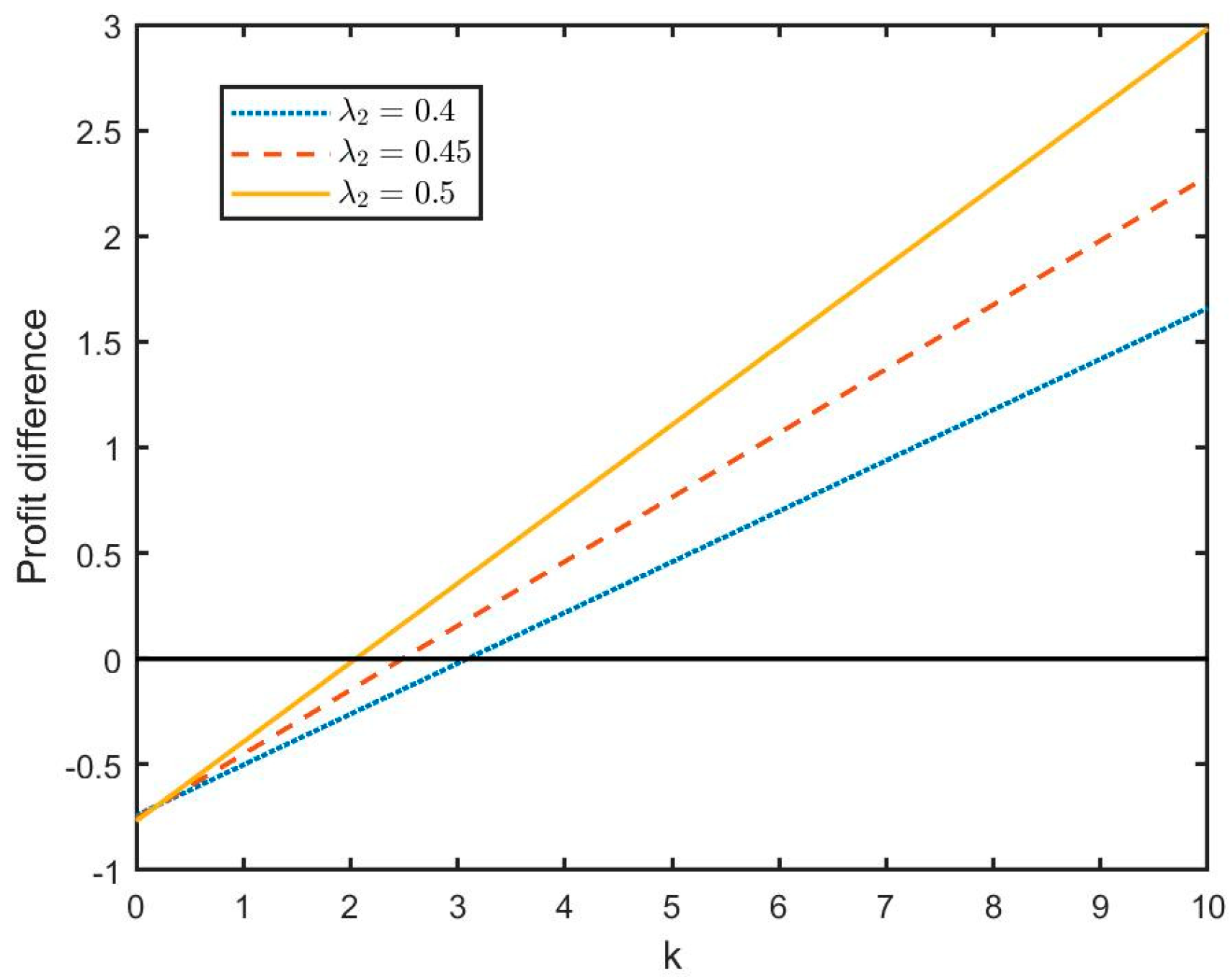
Corollary 3 demonstrates that the manufacturer will consider the coefficient of collection investment costs for external collection or in-house collection. In the case of no blockchain, the manufacturer can obtain a higher profit in Model BB if the coefficient of collection investment costs exceeds the threshold value (i.e., $k>k_0$). The reason is that the collection investment costs are larger than the purchase costs of product 2. At this time, the manufacturer is inclined to introduce collector 2 for product 2’s collection. Conversely, when the coefficient of collection investment costs is smaller, the manufacturer prefers the in-house collection (see Figure 2 for illustration). In the case of adopting blockchain, similarly, external collection can provide the manufacturer with the most profit increase when the coefficient of collection investment costs is higher than the threshold value $k_1$ (see Figure 3 for illustration). From Figure 2 and Figure 3, it can be seen that the collection rate affects the preference degree of the manufacturer’s recycling decision. The higher the recycling rate, the more likely the manufacturer is to choose external collection.

4.2. Comparison of Different Blockchain Adoption

In this subsection, we compare the equilibrium outcomes of different blockchain scenarios under the same collection scenario. From the viewpoint of optimal blockchain adoption, we compare the equilibrium outcomes. The results are summarized in Corollaries 4–6.

Corollary 4.

The optimal transfer prices and selling quantities satisfy the relations as follows: (i) For the transfer price, we can get $E[b_1^{AB}]>b_1^{AN}$, $E[b_1^{BB}]>E[b_1^{BN}]$ and $E[b_2^{BB}]>E[b_2^{BN}]$. (ii) For the selling quantities, we can get $E[q_i^{AB}]>E[q_i^{AN}]$ and $E[q_i^{BB}]>E[q_i^{BN}] (i=1,2)$.

Corollary 4 articulates that the optimal transfer prices and selling quantities with blockchain are larger than that in the case of no blockchain. When the supply chain members introduce the blockchain, consumers can obtain the key information on remanufactured products, which improves the consumer’s trust and expands the consumer market. Therefore, the selling quantities in the case of blockchain are larger than those without blockchain, as the increased selling quantities would stimulate collectors to increase the transfer prices. Hence, no matter the collection mode, the transfer prices and selling quantities with blockchain are higher than without blockchain. This means that the blockchain scenario benefits the improvement of both transfer prices and selling quantities.

Corollary 5.

By comparing the collectors’ expected profits in the same collection scenario, we find that $E[{\pi }_{R1}^{AB}]>E[{\pi }_{R1}^{AN}]$, $E[{\pi }_{R1}^{BB}]>E[{\pi }_{R1}^{BN}]$ and $E[{\pi }_{R2}^{BB}]>E[{\pi }_{R2}^{BN}]$.

Corollary 5 reveals that collectors can always benefit from blockchain technology. In the case of no blockchain, collectors do not have the full demand information and need to predict the uncertain demand based on the existing random information. When blockchain exists, collectors can obtain accurate demand from the blockchain. Thus, collectors have an extra demand information, which benefits the increase in collectors’ profit. Furthermore, according to Corollary 4, the transfer prices and selling quantities with blockchain are larger than that without blockchain. It is easy to conclude that collector 1 and collector 2’s profits in the case of blockchain are higher than that without blockchain.

Corollary 6.

By comparing the manufacturer’s expected profits in four models, we find that the manufacturer’s preference for blockchain depends on the variance of uncertain demand: (i) There exists a threshold $V_1$: if $V<V_1$, we have $E[{\pi }_M^{AB}]-E[{\pi }_M^{AN}]>0$. Otherwise, if $V>V_1$, we have $E[{\pi }_M^{AB}]-E[{\pi }_M^{AN}]<0$. (ii) There exists a threshold $V_2$: if $V<V_2$, we have $E[{\pi }_M^{BB}]-E[{\pi }_M^{BN}]>0$. Otherwise, if $V>V_2$, we have $E[{\pi }_M^{BB}]-E[{\pi }_M^{BN}]<0$.

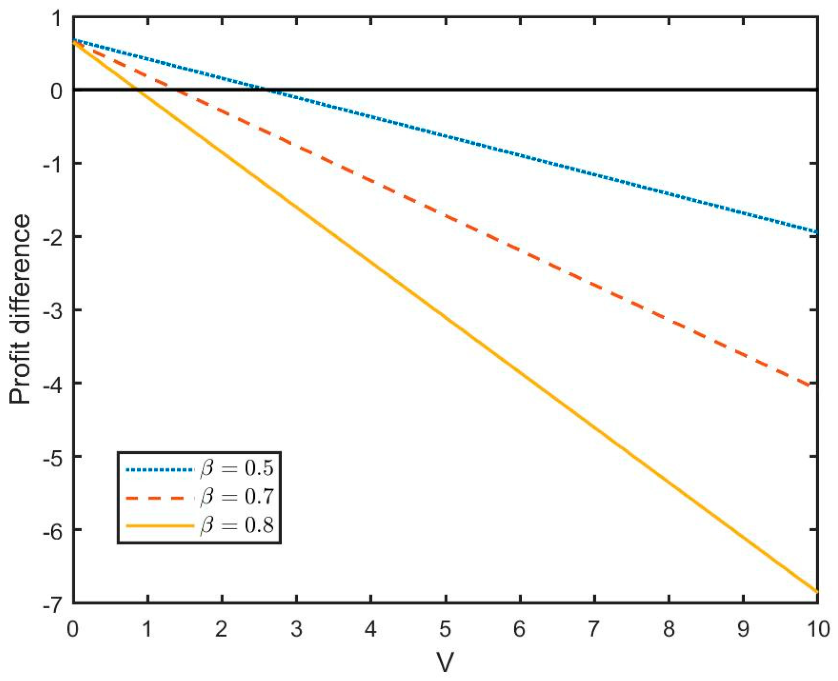
Corollary 6 illustrates that the variance in demand is one of the main factors that affect manufacturers in deciding whether to introduce blockchain technology. In Scenario A, the remanufacturing supply chain contains collector 1 and the manufacturer. When the demand variance is lower than a threshold value (i.e., $V<V_1$), the manufacturer is willing to introduce blockchain in order to expand the consumer market. When blockchain exists, the manufacturer records the demand information in the blockchain, which will provide collector 1 with accurate information about the market demand. Even though the manufacturer loses some demand information value, the increase in profits more than compensates for this loss. When the demand variance exceeds the threshold value (i.e., $V>V_1$), the demand information has a greater value than the profit increase. As a result, the manufacturer is unwilling to adopt blockchain (see Figure 4 for illustration). As shown in Figure 5, the manufacturer’s blockchain decision is also influenced by a threshold value in Scenario B. When the demand variance exceeds the threshold value (i.e., $V>V_2$), the manufacturer has a higher demand information value than the improvement of profit and prefers no blockchain. When the demand variance is lower than a threshold value (i.e., $V<V_2$), blockchain adoption can make the manufacturer obtain more profit from market expansion. Based on Figure 4 and Figure 5, it can be seen that there is a certain influence of the competition coefficient on the manufacturer’s recycling decisions. The manufacturer is more likely to adopt blockchain technology as competition increases.

5. Consumer Surplus

Consumer surplus is critically important for enterprises’ sustainable development. In this section, this study analyzes consumer surplus in different recycling models without blockchain. Followed by Yang et al. [39] and Shen et al. [40], the consumer utility function and consumer surplus are as follows:

$$U(q_1^{*},q_2^{*})={\varphi }_1{q}_1^{*}+{\varphi }_2{q}_2^{*}-\frac{{\psi }_1{q}_1^{*2}+2\gamma q_1^{*}{q}_2^{*}+{\psi }_2{q}_2^{*2}}{2}$$

(12)

$$CS=U\left(q_1^{*},q_2^{*}\right)-p_1^{*}{q}_1^{*}-p_2^{*}{q}_2^{*}$$

(13)

where the inverse demand functions are $p_1={\varphi }_1-{\psi }_1{q}_1-\gamma q_2$ and $p_2={\varphi }_2-{\psi }_2{q}_2-\gamma q_1$, respectively. Combining Equation (1) of the inverse demand function, we have ${\varphi }_1={\varphi }_2=a_N,{\psi }_1={\psi }_2=1,\gamma =\beta$. Therefore, the consumer surplus equation of this chapter can be derived as follows:

$$CS=a_N(q_1^{*}+q_2^{*})-\frac{q_1^{*2}+2\beta q_1^{*}{q}_2^{*}+q_2^{*2}}{2}-p_1^{*}{q}_1^{*}-p_2^{*}{q}_2^{*}=\frac{1}{2}\left(q_1^{*2}+2\beta q_1^{*}{q}_2^{*}+q_2^{*2}-2q_1^{*}{\epsilon }_1-2q_2^{*}{\epsilon }_2\right)$$

(14)

Corollary 7.

For the consumer, the higher the recycling rate of the product, the more benefits the consumer can get, and the consumer surplus increases.

Corollary 7 shows that the higher the collection rate, the more favorable the increase in consumer surplus. The optimal price of product 1 in Model AN is easily obtained $p_1^{AN}=\frac{\left(3-\beta \right)a_N+\left(1+\beta \right)c_m+2{\epsilon }_1-\Delta \left({\lambda }_1+\beta {\lambda }_2\right)}{4}$ and $p_2^{AN}=\frac{1}{2}\left(a_N+c_m+{\epsilon }_2-\Delta {\lambda }_2\right)$. It is easy to get $\frac{\partial p_1^{AN}}{\partial {\lambda }_i}<0 (i=1,2)$ and $\frac{\partial p_2^{AN}}{\partial {\lambda }_2}<0$. The first-order condition of the retail price in Model AN with respect to the collection rate shows that the retail price of the product decreases as the collection rate increases. The higher the product collection rate, the lower the retail price and the increase in consumer surplus. Therefore, for Model AN, the higher the collection rate, the higher the consumer surplus. In Model BN, the retail price of product 1 is $p_1^{BN}=\frac{\left(2+\beta \right)\left(3-2\beta \right)a_N+\left(2+\beta \right)c_m+\left(4-{\beta }^2\right){\epsilon }_1-\Delta \left(2{\lambda }_1+\beta {\lambda }_2\right)}{2\left(4-{\beta }^2\right)}$, the retail price of product 2 is $p_2^{BN}=\frac{\left(2+\beta \right)\left(3-2\beta \right)a_N+\left(2+\beta \right)c_m+\left(4-{\beta }^2\right){\epsilon }_2-\Delta \left(\beta {\lambda }_1+2{\lambda }_2\right)}{2\left(4-{\beta }^2\right)}$. The first order derivative of the collection rate for the optimal retail price are $\frac{\partial p_1^{BN}}{\partial {\lambda }_i}<0$ and $\frac{\partial p_2^{BN}}{\partial {\lambda }_i}<0 (i=1,2)$. It is easy to know that the higher the product collection rate, the lower the retail price of the product. For consumers, it is possible to purchase the remanufactured product at a lower retail price, which results in more benefits to consumers and an increase in consumer surplus. Therefore, for Model BN, the higher the product collection rate, the higher the consumer surplus.

6. Conclusions

In this paper, we examine the tradeoffs between different recycling strategies and blockchain adoption in a collector-led remanufacturing supply chain. The manufacturer has private demand information and has two different recycling strategies: in-house collection by the manufacturer or external collection by collector 2. There are four models for the recycling strategies and blockchain adoption: (1) Scenario A with no blockchain (Model AN); (2) Scenario B with no blockchain (Model BN); (3) Scenario A with blockchain (Model AB); (4) Scenario B with blockchain (Model BB). By comparing four models, we examine supply chain members’ preferences for collection formats and blockchain adoption. The main findings of this paper are as follows.

First, our study investigates the effect of the collection rate on the equilibrium solutions in different models. The unit transfer prices decrease with the increase in the collection rate in the four models. The selling quantities of product 1 are monotonically increasing in the collection rate ${\lambda }_1$ and decreasing in the collection rate ${\lambda }_2$. Similarly, the selling quantities of product 2 increase with ${\lambda }_2$ and decrease with ${\lambda }_1$. Product 1 and product 2 compete with each other in the same market, and competitors’ high collection rates are not conducive to their own selling quantities and profits. Collector 1’s (Collector 2’s) expected profits are increasing in ${\lambda }_1$ (${\lambda }_2$) only when the coefficient of collection investment costs is lower than a threshold value. The manufacturer’s expected profits are increasing in the two collection rates when external collection exists (Scenario B). However, In Scenario A, the manufacturer’s expected profits are increasing in ${\lambda }_2$ only when the coefficient of collection investment costs is lower than a threshold value.

Based on the above findings, there are some discussions and implications for this study. Product 1 and Product 2 compete with each other in the market; collectors do not want competitors’ collection rates to increase. However, it is not that the higher the collection rate of its own products, the higher its own profit value. Collectors need to make a cost investment in recycling channels. Only when the coefficient of collection investment cost is lower than a threshold value can a higher product collection rate increase the collectors’ profits. Therefore, it is necessary for collectors to consider the improvement of product collection rate and control the cost of collection investment. For the manufacturer, the higher the product collection rate under external collection mode, the better the benefits. However, the manufacturer needs to control the cost of collection investment while considering increasing the collection rate of product 2 under in-house collection.

Second, we compare the differences in the equilibrium solutions of different models. The unit transfer prices and the selling quantities of product 1 in Scenario B are higher than in Scenario A. Moreover, the unit transfer prices and selling quantities of product 1 and product 2 with blockchain are higher than that without blockchain. However, the selling quantities of product 2 in Scenario B are lower than in Scenario A. Both collector 1 and collector 2 are willing to adopt blockchain in the remanufacturing supply chain. In the case of no blockchain, collector 1 is always inclined to the manufacturer to introduce external collection by collector 2. However, collector 1 prefers Scenario B with blockchain only when demand variance and the coefficient of variance are larger than a threshold value (i.e., $V>V_0$ and $r>r_0$). The manufacturer’s decision on in-house collection and external collection depends on the coefficient of collection investment costs. Only when the coefficient of collection investment costs exceeds a certain value with/without blockchain will the manufacturer choose external collection; otherwise, the manufacturer prefers in-house collection. The manufacturer may choose to implement the blockchain when the demand variance is less than a certain value.

The findings of the second part have some inferences and implications. Collectors are looking to introduce blockchain technology to record information about remanufactured products. Not only can they gain accurate demand information value, but they can also obtain greater sales from blockchain technology that improves consumer trust in remanufactured products. However, the manufacturer is willing to introduce blockchain technology only when the variance of demand is smaller than a threshold value. Therefore, we recommend that the remanufacturing supply chain jointly introduce blockchain technology when the variance of demand is small so that a win-win situation can be achieved. In the case of blockchain, the manufacturer and collector 1 prefer external collection only if both the variance indicator of demand and the coefficient of collection investment costs meet a certain range.

Finally, our research expands the theoretical perspective and provides practical guidance. This study reveals the impact of demand randomization and blockchain technology on recycling strategies in a collector-led remanufacturing supply chain and enriches the theoretical research on the impact of uncertainties on the remanufacturing supply chain’s operation decision. At the same time, it also provides a practical guide for the introduction of blockchain technology in the remanufacturing supply chain.

Furthermore, this paper has several limitations, which can be considered for future research. First, this study does not distinguish between new and remanufactured products. In some situations, remanufactured products do not meet the same quality standards as new products. Thus, it would be possible to study the scenario of remanufactured products that are differentiated in the future. Second, we assume that all participants are risk-neutral under uncertain demand and do not take into account their risk attitudes. The risk attitudes of heterogeneous players may vary in practice. Third, the product collection rate was not set as a decision variable in this study. In fact, product recovery rates are not fixed constants. Considering making the collection rate a decision variable is also a direction for future research. In the future, the above issues may prove to be interesting.

References

1. Yang, L.; Gao, M.; Feng, L. Competition versus cooperation? Which is better in a remanufacturing supply chain considering blockchain. Transp. Res. E-Logist. Transp. Rev. 2022, 165, 102855. [Google Scholar] [CrossRef]
2. Han, X.; Yang, Q.; Shang, J.; Pu, X. Optimal strategies for trade-old-for-remanufactured programs: Receptivity, durability, and subsidy. Int. J. Prod. Econ. 2017, 193, 602–616. [Google Scholar] [CrossRef]
3. Wu, X.; Zhou, Y. The optimal reverse channel choice under supply chain competition. Eur. J. Oper. Res. 2017, 259, 63–66. [Google Scholar] [CrossRef]
4. Savaskan, R.C.; Van Wassenhove, L.N. Reverse Channel Design: The Case of Competing Retailers. Manag. Sci. 2006, 52, 1–14. [Google Scholar] [CrossRef]
5. Cai, K.; Zhang, Y.; Lou, Y.; He, S. Information sharing in a collectors-led closed-loop supply chain. RAIRO-Oper. Res. 2022, 56, 2329–2350. [Google Scholar] [CrossRef]
6. Yang, F.; Wang, M.; Ang, S. Optimal remanufacturing decisions in supply chains considering consumers’ anticipated regret and power structures. Transp. Res. E-Logist. Transp. Rev. 2021, 148, 102267. [Google Scholar] [CrossRef]
7. Krikke, H.; Hofenk, D.; Wang, Y. Revealing an invisible giant: A comprehensive survey into return practices within original (closed-loop) supply chains. Resour. Conserv. Recycl. 2013, 73, 239–250. [Google Scholar] [CrossRef]
8. Ovchinnikov, A. Revenue and Cost Management for Remanufactured Products. Prod. Oper. Manag. 2011, 20, 824–840. [Google Scholar] [CrossRef]
9. Aydin, R.; Mansour, M. Investigating sustainable consumer preferences for remanufactured electronic products. J. Eng. Res. 2023, 11, 100008. [Google Scholar] [CrossRef]
10. Yue, X.; Liu, J. Demand forecast sharing in a dual-channel supply chain. Eur. J. Oper. Res. 2006, 174, 646–667. [Google Scholar] [CrossRef]
11. Huang, Y.; Wang, Z. Information sharing in a closed-loop supply chain with technology licensing. Int. J. Prod. Econ. 2017, 191, 113–127. [Google Scholar] [CrossRef]
12. Choi, T.M. Blockchain-technology-supported platforms for diamond authentication and certification in luxury supply chains. Transp. Res. E-Logist. Transp. Rev. 2019, 128, 17–29. [Google Scholar] [CrossRef]
13. Yanikoglu, I.; Denizel, M. The value of quality grading in remanufacturing under quality level uncertainty. Int. J. Prod. Res. 2021, 59, 839–859. [Google Scholar] [CrossRef]
14. Abbey, J.D.; Kleber, R.; Souza, G.C.; Voigt, G. Remanufacturing and consumers’ risky choices: Behavioral modeling and the role of ambiguity aversion. J. Oper. Manag. 2019, 65, 4–21. [Google Scholar] [CrossRef]
15. Gong, B.; Zhang, H.; Gao, Y.; Liu, Z. Blockchain adoption and channel selection strategies in a competitive remanufacturing supply chain. Comput. Ind. Eng. 2023, 175, 108829. [Google Scholar] [CrossRef]
16. Niu, B.; Xu, H.; Chen, L. Creating all-win by blockchain in a remanufacturing supply chain with consumer risk-aversion and quality untrust. Transp. Res. E-Logist. Transp. Rev. 2022, 163, 102778. [Google Scholar] [CrossRef]
17. Zhang, T.Y.; Dong, P.W.; Chen, X.F.; Gong, Y. The impacts of blockchain adoption on a dual-channel supply chain with risk-averse members. Omega-Int. J Manag. Sci. 2023, 114, 102747. [Google Scholar] [CrossRef]
18. Cui, Y.; Hu, M.; Liu, J.C. Value and Design of Traceability-Driven Blockchains. MSom-Manuf. Serv. Oper. Manag. 2023, 1–18, Article in advance. [Google Scholar] [CrossRef]
19. Zheng, Y.; Xu, Y.Q.; Qiu, Z.G. Blockchain Traceability Adoption in Agricultural Supply Chain Coordination: An Evolutionary Game Analysis. Agriculture 2023, 13, 184. [Google Scholar] [CrossRef]
20. Wang, C.F.; Chen, X.F.; Xu, X.; Jin, W. Financing and operating strategies for blockchain technology-driven accounts receivable chains. Eur. J. Oper. Res. 2023, 304, 1279–1295. [Google Scholar] [CrossRef]
21. Huang, Y.D.; Widyadana, G.A.; Wee, H.M.; Blos, M.F. Revenue and risk sharing in view of uncertain demand during the pandemics. Rairo-Oper. Res. 2022, 56, 1807–1821. [Google Scholar] [CrossRef]
22. Ji, C.Y.; Liu, X.X. Design of risk sharing and coordination mechanism in supply chain under demand and supply uncertainty. Rairo-Oper. Res. 2022, 56, 123–143. [Google Scholar] [CrossRef]
23. Garai, T.; Paul, A. The effect of supply disruption in a two-layer supply chain with one retailer and two suppliers with promotional effort under random demand. J. Manag. Anal. 2022, 10, 22–37. [Google Scholar] [CrossRef]
24. Li, Y.C.; Saldanha-da-Gama, F.; Liu, M.; Yang, Z.L. A risk-averse two-stage stochastic programming model for a joint multi-item capacitated line balancing and lot-sizing problem. Eur. J. Oper. Res. 2023, 304, 353–365. [Google Scholar] [CrossRef]
25. Pei, H.L.; Liu, Y.K.; Li, H.L. Robust Pricing for a Dual-Channel Green Supply Chain Under Fuzzy Demand Ambiguity. IEEE Trans. Fuzzy Syst. 2023, 31, 53–66. [Google Scholar] [CrossRef]
26. Liu, W.J.; Liu, W.; Shen, N.N.; Xu, Z.T.; Xie, N.M.; Chen, J.; Zhou, H.Y. Pricing and collection decisions of a closed-loop supply chain with fuzzy demand. Int. J. Prod. Econ. 2022, 245, 108409. [Google Scholar] [CrossRef]
27. Zheng, B.R.; Wen, K.; Jin, L.; Hong, X.P. Alliance or cost-sharing? Recycling cooperation mode selection in a closed-loop supply chain. Sustain. Prod. Consum. 2022, 32, 942–955. [Google Scholar] [CrossRef]
28. Long, X.F.; Ge, J.L.; Shu, T.; Liu, Y. Analysis for recycling and remanufacturing strategies in a supply chain considering consumers’ heterogeneous WTP. Resour. Conserv. Recycl. 2019, 148, 80–90. [Google Scholar] [CrossRef]
29. Yi, P.X.; Huang, M.; Guo, L.J.; Shi, T.L. Dual recycling channel decision in retailer oriented closed-loop supply chain for construction machinery remanufacturing. J. Clean. Prod. 2016, 137, 1393–1405. [Google Scholar] [CrossRef]
30. Huang, M.; Yi, P.X.; Shi, T.L. Triple Recycling Channel Strategies for Remanufacturing of Construction Machinery in a Retailer-Dominated Closed-Loop Supply Chain. Sustainability 2017, 9, 2167. [Google Scholar] [CrossRef]
31. Zhang, W.S.; Zhang, T. Recycling channel selection and financing strategy for capital-constrained retailers in a two-period, closed-loop supply chain. Front. Environ. Sci. 2022, 10, 1–16. [Google Scholar] [CrossRef]
32. He, Q.D.; Wang, N.M.; Browning, T.R.; Jiang, B. Competitive collection with convenience-perceived customers. Eur. J. Oper. Res. 2022, 303, 239–254. [Google Scholar] [CrossRef]
33. Guo, Y.; Wang, M.M.; Yang, F. Joint emission reduction strategy considering channel inconvenience under different recycling structures. Comput. Ind. Eng. 2022, 169, 108159. [Google Scholar] [CrossRef]
34. Wan, N.A. Impacts of sales mode and recycling mode on a closed-loop supply chain. Int. J. Syst. Sci. 2023, 54, 1–22. [Google Scholar] [CrossRef]
35. Cao, H.Q.; Ji, X.F. Optimal Recycling Price Strategy of Clothing Enterprises based on Closed-loop Supply Chain. J. Ind. Manag. Optim. 2023, 19, 1350–1366. [Google Scholar] [CrossRef]
36. Yang, T.J.; Li, C.M.; Yue, X.P.; Zhang, B.B. Decisions for Blockchain Adoption and Information Sharing in a Low Carbon Supply Chain. Mathematics 2022, 10, 2233. [Google Scholar] [CrossRef]
37. Niu, B.Z.; Dong, J.; Liu, Y.Q. Incentive alignment for blockchain adoption in medicine supply chains. Transp. Res. E-Logist. Transp. Rev. 2021, 152, 32. [Google Scholar] [CrossRef]
38. Shi, C.-l.; Geng, W.; Sheu, J.-B. Integrating dual-channel closed-loop supply chains: Forward, reverse or neither? J. Oper. Res. Soc. 2020, 72, 1844–1862. [Google Scholar] [CrossRef]
39. Yang, X.D.; Cai, G.S.; Ingene, C.A.; Zhang, J.H. Manufacturer Strategy on Service Provision in Competitive Channels. Prod. Oper. Manag. 2020, 29, 72–89. [Google Scholar] [CrossRef]
40. Shen, B.; Zhu, C.; Li, Q.; Wang, X. Green technology adoption in textiles and apparel supply chains with environmental taxes. Int. J. Prod. Res. 2020, 59, 4157–4174. [Google Scholar] [CrossRef]
Figure 1. Supply chain structures.
Processes 11 01426 g001
Figure 2. The impact of k on profit difference. ( a N = 2 ,   c m = 1.5 ,   Δ = 0.5 ,   r = 0.8 ,   β = 0.5 ,   ϕ = 1.5 ,   λ 1 = 0.6 ).
Processes 11 01426 g002
Figure 3. The impact of k on profit difference. ( a B = 3 ,   c m = 1.5 ,   Δ = 0.5 ,   r = 0.8 ,   β = 0.5 ,   ϕ = 1.5 ,   λ 1 = 0.6 ).
Processes 11 01426 g003
Figure 4. The impact of k on profit difference. ( a B = 3 ,   a N = 2 , c m = 1.5 ,   Δ = 0.5 ,   r = 0.8 ,   λ 1 = 0.6 , λ 2 = 0.5 ).
Processes 11 01426 g004
Figure 5. The impact of k on profit difference. ( a B = 3 ,   a N = 2 , c m = 1.5 ,   Δ = 0.5 ,   r = 0.8 ,   λ 1 = 0.6 , λ 2 = 0.5 ).
Processes 11 01426 g005