Article

Recognition of Timestamps and Reconstruction of the Line of Organism Development

by
Andrzej Kasperski
Laboratory of Bioinformatics and Control of Bioprocesses, Institute of Biological Sciences, Department of Biotechnology, University of Zielona Góra, ul. Szafrana 1, 65-516 Zielona Góra, Poland
Processes 2023, 11(5), 1316; https://doi.org/10.3390/pr11051316
Submission received: 20 March 2023 / Revised: 4 April 2023 / Accepted: 13 April 2023 / Published: 24 April 2023
(This article belongs to the Special Issue Computational Biology Approaches to Genome and Protein Analyzes)

Abstract

:
In this work, an artificial neural network is used to recognize timestamps of evolution. Timestamps are associated with outliers determined during the recognition of the genome attractors of organisms. The aim of this work is to present a new method of penetrating deep into evolution using the recognized timestamps. To achieve this aim, the neural networks of different number of layers were implemented in order to check the influence of the number of layers on the visibility of the timestamps. Moreover, the teaching process was repeated 10 times for each implemented neural network. The recognition of each organism evolution was also repeated 10 times for each taught neural network to increase the reliability of the results. It is presented, among other findings, that during the recognition of the timestamps of evolution not only the number of homologous comparisons and the lengths of compared sequences are important but also the distribution of similarities between sequences. It is also presented that the recognized timestamps allow for travel between genome attractors and reconstruct the line of organism development from the most advanced to the most primitive organisms. The results were validated by determining timestamps for exemplary sets of organisms and also in relation to semihomology approach and by phylogenetic tree generation.

1. Introduction

The genetic history of organism development is stored in the cell genome [1,2]. This phenomenon is called phylogenetic memory [1,2]. The existence of a phylogenetic memory can indicate that there are genes in the genome that represent the evolutionary genetic history of organisms. These genes should also allow for the recognition of the timestamps of organism development. An example of the existence of phylogenetic memory is cancer development. The transformed cell loses control over this historic potential stored in the genome, and as a result, the atavistic code is activated uncontrollably [3,4]. This article is an extension of previously published works that present unified cell bioenergetics (UCB) and propose methods that can be used to study organism evolution [4,5,6,7,8,9,10]. It has been pointed out that UCB allows for the interpretation of several cell bioenergetic effects, certain diseases and as well as some causes of evolution [10,11,12,13,14,15]. As it was presented, the evolution of organisms can be considered as a discontinuous process that occurs mainly in genome attractors, where organisms undergo random mutations and natural selection [5,16,17]. In a general sense, the term “attractor” denotes a configuration to which the system tends over time. After attaining the attractor, the system gains sufficient stability to return to its original state after the disappearance of emerging disturbances [18]. In this sense, genome attractors allow for the stabilization of configurations of features that are typical for given organisms [5]. This approach is consistent with the researchers’ current interest in ‘organisms as attractors in phase space’ [19].
As a highly conserved and omnipresent protein, cytochrome c is additionally characterized by linear changes in amino-acid differences between different lineages over time, which makes it suitable for the study of cladistics [20,21,22]. In this work, cytochrome c is used as a representative that allows not only for the recognition of genome attractors, but also keeps historical information about organism evolution. This historical information can be considered as specific pictures that have been written in DNA during organism evolution. In this work, is presented what is visible during the analysis of these evolutionary pictures and how deep we can penetrate into evolution using these pictures. As it is presented, these pictures can be recognized by artificial neural networks and, based on this recognition, the timestamps of evolution can be identified. As a result, in this work a new method of penetrating deep into evolution using the recognized timestamps has been established. It is presented that, using this method, traveling between genome attractors and the reconstruction of the line of organism development from the most advanced to the most primitive organisms is possible.
Modern methods of determining phylogeny are usually based on calculations. Phylogenetic trees have remained a central metaphor in evolutionary biology since Charles Darwin sketched his first evolutionary tree in 1837 [23]. Evolutionary trees have now become the subject of detailed, rigorous study to reconstruct the branching patterns that led to the diversity of life evolution [23,24,25]. The fundamental problem in striving to determine the real course of evolution by generating phylogenetic trees is the very large number of trees (even for a relatively small number of taxa) that should be evaluated in order to select the tree that can be considered the best in the light of the assumed criteria [26]. For this reason, the determination of the best tree must very often be made after evaluating a small number of possible trees. In this case, along with determining the best tree, it is necessary to determine the reliabilities of internal nodes in the tree. One of the most commonly used methods to determine the reliability of a generated tree is the bootstrap method, which uses the bootstrap resampling technique [27,28]. The bootstrap method has been implemented, for example, in the MEGA program [29]. A small number of evaluated trees, in relation to the total number of trees that can be generated, can be considered as an important factor of the low reliability of tree nodes. Especially in the case when nodes of low reliability are located close to the root of the tree, the reliability of the entire generated tree can also be considered low. This disadvantage of using phylogenetic trees to reconstruct the real phylogenesis makes it necessary to develop and implement new algorithms dedicated, among others, to reconstruct the line of organism development.
Artificial neural networks (ANNs) are a method of artificial intelligence that has been applied in various fields [30,31,32,33,34]. ANNs are most suitable for solving complex, highly non-linear, ill-defined problems with many different variables, which include, for example, establishing protein secondary structure, classification of cancers, gene prediction and drug design [30,35,36]. In this work, neural networks are used to recognize patterns drawn by evolution (and stored in cytochromes c), but contrary to previous works, genome attractors were not exclusively detected. The aim of this work is to show how to reconstruct the line of organism development using the timestamps of evolution recognized by artificial neural networks.
This article is organized as follows: First, the methods and theoretical bases are presented, including descriptions of the implemented neural networks along with teaching and recognition procedures and a semihomologous approach. Secondly, a new method of penetrating deep into evolution using the recognized timestamps is presented for the exemplary organisms along with the validation of the results. Then, a general algorithm of the method of penetrating deep into evolution, with the aim to establish a line of organism development, is proposed. Finally, the conclusions are presented.

2. Materials and Methods

At the beginning of this section, the web resources and programs used in this study are discussed, followed by information related to the artificial neural networks (i.e., implementation, teaching and recognition), as well as the semihomologous approach.

2.1. Web Resources

The cytochrome c amino-acid sequences selected for this study were downloaded from the NCBI and UniProt databases (http://staff.uz.zgora.pl/akaspers/Pro/sequences.txt (accessed on 20 March 2023)).

2.2. Computer Programs

The calculations presented in this work were made using the EvolutionXXI, dotPicker and MEGA X programs. The EvolutionXXI and dotPicker programs were written by the author. The EvolutionXXI contains an implemented neural network and was used in this work to recognize timestamps. The dotPicker program contains an implemented multidimensional semihomologous Dot-Matrix method and was used in this work to determine similarities between sequences at the codon level. The MEGA X program [29] was used to generate phylogenetic trees.

2.3. Implementation and Teaching of the Artificial Neural Networks

Neural networks with different numbers of layers were implemented, (i.e., neural networks with 2, 3, 4, 5, 6, 7 and 8 layers) in order to check the impact of the number of layers on the teaching process and results. In the first step of the research, each of the implemented neural networks was taught 10 times using a set of 15 organisms (see Table 1). The recognition of each organism was also repeated 10 times and the final result of recognition was calculated as an average value in order to increase the reliability of the results. A standard deviation was calculated for each final recognition result. A low standard deviation means that there are data clusters around the mean. A high standard deviation indicates that the data are widely spread out.
Full-synapse ANNs with the sigmoid transfer function y = 1/(1 + exp(−x)) were implemented and taught [37,38,39]. The amino-acid sequences used to teach and recognize organism evolution were converted to binary form by changing each character in the sequences to a five-positional binary number (i.e., ‘A’ was converted to “00001”, ‘B’ was converted to “00010” and ‘C’ was converted to “00011”). This way of conversion offered good results when cytochrome b and cytochrome c sequences were used to recognize evolution [5,6]. All sequence lengths were adjusted to 105 (since the number of amino acids in cytochrome c sequences is approximately 105) by cutting the sequence or adding “−” characters encoded by “00000” when the sequence was longer or shorter, respectively [5]. After alignment, the length binary form of sequences was equal to 5 × 10⁵, which determines the number of neurons in the ANN input layer (i.e., nbrInp = 525) [5]. The number of neurons in the ANN output layer was equal to the number of organisms. The number of neurons in the hidden layers was established by the geometric pyramid rule [40]. In accordance with the geometric pyramid rule, the number of neurons in the hidden layers is equal to:
For one hidden layer:
nbrHid = ( nbrInp × nbrOut ) 1 2
nbrHid—the number of neurons in the hidden layer;
nbrInp—the number of neurons in the input layer;
nbrOut—the number of neurons in the output layer.
For two hidden layers:
r = ( nbrInp / nbrOut ) 1 3
nbrHid 1 = nbrOut   ×   r 2     the   number   of   neurons   in   the   first   hidden   layer ;
nbrHid 2 = nbrOut   ×   r     the   number   of   neurons   in   the   sec ond   hidden   layer .
For three hidden layers:
r = ( nbrInp / nbrOut ) 1 4
nbrHid 1 = nbrOut   ×   r 3     the   number   of   neurons   in   the   first   hidden   layer ;
nbrHid 2 = nbrOut   ×   r 2     the   number   of   neurons   in   the   sec ond   hidden   layer ;
nbrHid 3 = nbrOut   ×   r     the   number   of   neurons   in   the   third   hidden   layer .
and so on.
The number of neurons in the layers of the implemented neural networks for the 15 organisms used for teaching, calculated in accordance with the geometric pyramid rule, is presented in Table 2. The number of neurons in each layer, for example, for 5-layer neural network, is equal to: nbrInp = 525, nbrHid1 = 216, nbrHid2 = 89, nbrHid3 = 36, nbrOut = 15.
Before teaching, the 15 organisms (Table 1) were set in random order. A teaching pattern for the first organism was equal to “000000000000001”, for the second organism “000000000000010”, for the third organism “000000000000100”, and for the 15th organism “100000000000000”. ANNs were taught using the online backpropagation algorithm (learning rate equal to 0.3 and momentum equal to 0.1), using established patterns in this way. The teaching processes were carried out until the root-mean-squared Error (RMSE) was below 0.002. This way of teaching the ANN indicates that the recognition of organism similarities is in the range between 0 and 1, where 0 means the smallest similarity and 1 means the highest similarity. Calculations were made on a computer with the following characteristics: IBM HS23 (2CPU Xenon E5–2650 × 4 Core, 2.00 GHz, RAM = 12 GB, HDD = 50 GB.

2.4. Semihomologous Approach

The semihomologous approach allows for a better interpretation of the results, by allowing amino-acid comparison at the codon level [41,42,43]. If the compared amino-acids are different, the level of considerations is changed and the amino-acids are compared at the codon level. As a result, the result of the comparison of two amino-acid sequences can contain positions of the following types:
  • “R”—Homologous position, if the compared amino-acids are the same;
  • “#”—Transition-type semihomologous position, if there is a one-point mutation of the transition type in the codons of the compared amino-acids;
  • $”—Transversion-type semihomologous position, if there is a one-point mutation of the transversion type in the codons of the compared amino-acids;
  • “-”—Another position, if there is two or three point mutation in the codons of compared amino acids.

3. Results and Discussion

First, the neural networks were taught and validated and timestamps were recognized for sets of monkeys and fish. It transpired that, during the recognition, not only similarity to the closest evolutionary organism can be recognized but also similarities to other, evolutionarily more distant organisms, as similarities of the lower values visible in the “background”. In this article, a set of recognized outliers constitutes the timestamp of evolution. Background similarities usually have relatively small values, for this reason, it was decided to teach each neural network more than once (i.e., 10 times) to increase the reliability of outlier recognition. Each examined organism was also recognized 10 times by each taught neural network and the similarities presented in the article were calculated as the arithmetic means of 10 recognitions. The standard deviations were calculated and presented along with the average similarities.

3.1. Teaching of the Neural Networks

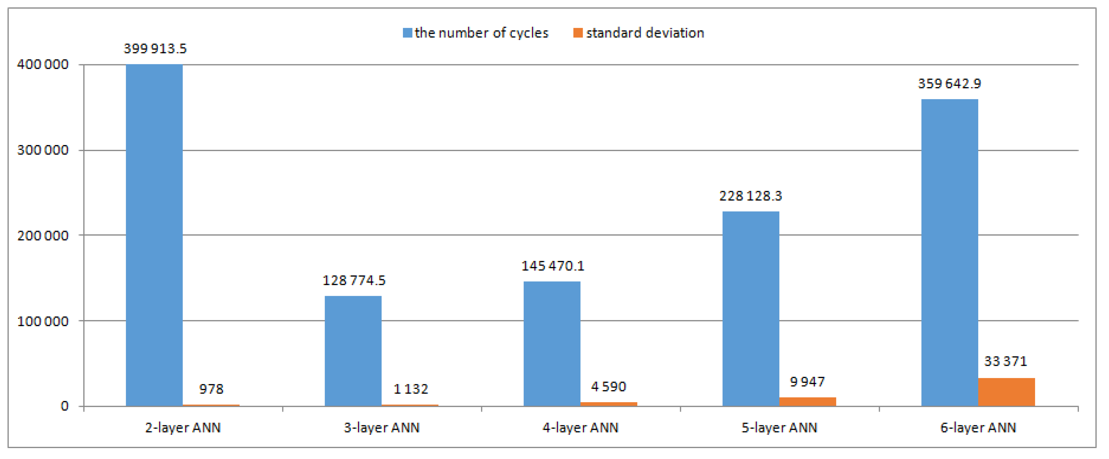
In general, the teaching process involves updating the weights of neurons [37]. In this work, the weights in the artificial neural networks (ANNs) were adjusted using the error (root-mean-squared Error (RMSE)) between the predicted and correct values in order to minimize RMSE (i.e., lower RMSE to a value below 0.002). It was concluded that it is impossible to teach an 8-layer neural network using the set of 15 organisms, i.e., after several days of teaching, the RMSE was higher than 0.5. Moreover, for a 7-layer neural network, only about 30% of the teaching processes conducted were successful (i.e., RMSE dropped below 0.002). For 2-, 3-, 4-, 5- and 6-layer neural networks, the teaching process was repeated 10 times. Figure 1 shows the average number of teaching cycles and standard deviations for processes of teaching the 2-, 3-, 4-, 5- and 6-layer neural networks.
From Figure 1, it can be observed that the 2-layer neural network needs the largest number of teaching cycles, but the standard deviation (of the number of teaching cycles) calculated for 10 teaching processes is the smallest. For a 3-layer ANN, the number of teaching cycles is the smallest. When the number of layers increases from 3 to 6, the number of teaching cycles and standard deviation increase; however, the standard deviation remains relatively small for a 5-layer ANN.

3.2. Validation of the Neural Networks and Recognition of Timestamps for a Set of Monkeys

First, the taught neural networks were validated using a set of monkeys. As shown in Table A1, Table A2, Table A3, Table A4 and Table A5 (see Appendix A), timestamps that contain three outliers (Homo sapiens, Horse and Crow (listed in the order of the decreasing average value of recognized similarity)) were recognized during this validation. This means that, when recognizing similarity, monkeys are similar to Homo sapiens, but also to Horse to a lesser extent and to Crow the least. That means that monkeys show, mainly, a similarity to Homo sapiens but that similarities to Horse and to Crow are also visible in “the background”. It is also evident that similarities to Homo sapiens recognized by 2-, 3-, 4- and 5-layer neural networks were greater than similarities recognized to Horse and any standard deviation was small (see Table A1, Table A2, Table A3 and Table A4 in Appendix A). Moreover, an increase in the number of layers from 2 to 5 caused an increase in similarity to Homo sapiens. For the 6-layer ANN, the similarity of New World Monkeys (i.e., monkeys with numbers from 12 to 18 (see Table A5 in Appendix A)) to Homo sapiens suddenly decreased, the similarity to Horse increased significantly and the standard deviation increased, compared to the 5-layer ANN. For this reason, the subsequent recognitions presented in this work were made using 2-, 3-, 4- and 5-layer ANNs.

3.3. Validation of the Neural Networks and Recognition of Timestamps for a Set of Fish

The neural networks were also validated using a set of fish. As shown in Table A6 and Table A9, the timestamps that contain five outliers (Horse, Crow, Frog, Goldfish and Worm) were recognized during this validation. The greatest similarities of each fish from the set of fish used for validation (i.e., Epinephelus moara, Epinephelus fuscoguttatus, Brienomyrus brachyistius, Hypomesus transpacificus and Nothobranchius furzeri) were to Goldfish by each neural network, i.e., by 2-, 3-, 4- and 5-layer ANNs (see Table A6 and Table A9 in Appendix A), which is in accordance with our expectations.
An especially interesting result was that for Nothobranchius furzeri. The recognized similarities of Nothobranchius furzeri to Goldfish by the 2-, 3-, 4- and 5-layer ANNs were equal to 0.83611, 0.57080, 0.60185 and 0.88947, respectively, and were greater than the similarities recognized to Frog, Crow, Horse and Worm (i.e., the other outliers) (see Table A6 and Table A9 in Appendix A). The number of homologous comparisons (i.e., the number of “R” positions) between Nothobranchius furzeri and Goldfish is equal to 91 (see Table A6 and Table A9 in Appendix A). The numbers of homologous comparisons between Nothobranchius furzeri and Frog, Crow and Horse were equal to 92, 98 and 95, respectively (see Table A6 and Table A9 in Appendix A). Therefore, considering only the number of homologous comparisons, it is impossible to detect that the similarity of Nothobranchius furzeri to Goldfish is the greatest. It means that, during the detection of evolutionary similarities, not only the number of homologous comparisons and the lengths of compared sequences are important, but also the distribution of similarities between the compared sequences.
In addition, this validation also showed that the greatest similarities to the closest evolutionary organism was recognized by the 5-layer ANN, i.e., the recognized similarities of each fish from the set of fish used for validation were the greatest for the 5-layer ANN (see Table A6 in Appendix A). For this reason, the 5-layer ANN was used to demonstrate the method of penetrating deep into evolution and reconstructing the line of organism development.

3.4. Method of Penetrating Deep into Evolution and Reconstruction of the Line of Organism Development

The recognized timestamps for a set of monkeys (see the Validation of the Neural Networks and Recognition of Timestamps for a Set of Monkeys Section) can indicate that the temporary line of development from the most advanced to the most primitive organisms begins with Homo sapiens and leads to two less developed organisms, i.e., to Horse and then Crow (see Table A1, Table A2, Table A3, Table A4 and Table A5 in Appendix A). Because the recognized timestamps for a set of monkeys contain only three outliers (Homo sapiens, Horse and Crow (see Table A1, Table A2, Table A3, Table A4 and Table A5 in Appendix A)), it is impossible to determine which is the next organism “hidden in the depths” of evolution.
The steps of the proposed method, which reveal the line of organism development from the most advanced to the most primitive organisms, are as follows:
(a)
In the first step of the proposed method, Homo sapiens, as the most developed organism, is recognized by the 5-layer neural network. The results of the recognition of Homo sapiens are presented in Table 3.
(b)
In the next step, the organism with the greatest recognized similarity (i.e., Homo sapiens) is removed from the set of organisms and the 5-layer neural network is taught using the remaining (fourteen) organisms. After re-teaching, the removed organism (i.e., Homo sapiens) is recognized once again. The new results of the recognition of Homo sapiens are presented in Table 4.
The recognized timestamp (a set of outliers) indicates that the removal of Homo sapiens caused the level of considerations to be shifted to less developed organisms, i.e., from the Homo sapiens genome attractor to the Horse genome attractor (with Crow and Frog genome attractors being visible in the background). It should be noted that the largest outlier (Horse) was recognized reliable, as evidenced by the relatively small value of the standard deviation (0.05320). The recognized timestamp indicates a temporary line of development from the most advanced to the most primitive organisms, i.e., Homo sapiens, Horse, Crow and Frog. The procedure was repeated in the next steps as follows. The organism with the greatest recognized similarity is removed from the set of organisms; the 5-layer neural network is taught using the remaining organisms; and, after re-teaching, the removed organism is recognized. The recognized timestamps indicate the temporary line of development from the most advanced to the most primitive organisms. It can be seen that, in general, the method is based on the principle that “it is necessary to approach the bend in order to see what is around the bend”.
(c)
In the next step, the organism with the greatest recognized similarity (i.e., Horse) is removed from the set of organisms and the 5-layer neural network is taught using the remaining (thirteen) organisms. After re-teaching, the removed organism (i.e., Horse) is recognized. The results of the recognition of Horse are presented in Table 5.
(d)
In the next step, the organism with the greatest recognized similarity (i.e., Crow) is removed from the set of organisms and the 5-layer neural network is taught using the remaining (twelve) organisms. After re-teaching, the removed organism (i.e., Crow) is recognized. The results of the recognition of Crow are presented in Table 6. In this case, the standard deviation associated with the recognized similarity Crow to Frog (i.e., the biggest outlier) is relatively large (recognized similarity equal to 0.57232 and standard deviation equal to 0.30661), which means that this similarity was not very clearly visible by the neural network.
(e)
In the next step, the organism with the greatest recognized similarity (i.e., Frog) is removed from the set of organisms and the 5-layer neural network is taught using the remaining (eleven) organisms. After re-teaching, the removed organism (i.e., Frog) is recognized. The results of the recognition of Frog are presented in Table 7.
(f)
The organism with the greatest recognized similarity (i.e., Goldfish) is removed from the set of organisms and the 5-layer neural network is taught using the remaining (ten) organisms. After re-teaching, the removed organism (i.e., Goldfish) is recognized. The results of the recognition of Goldfish are presented in Table 8.
(g)
In the next step, the organism with the greatest recognized similarity (i.e., Worm) is removed from the set of organisms and the 5-layer neural network is taught using the remaining (nine) organisms. After re-teaching, the removed organism (i.e., Worm) is recognized. The results of the recognition of Worm are presented in Table 9.
It is clear that, after this step, the line of organism development leads to Bacteria, which may indicate that the remaining organisms are located in other side branches (i.e., “side tracks” [23]) of the evolutionary tree having a small similarity to Worm. The standard deviation associated with the recognized similarity to Bacteria (and also associated with the recognition of the other outliers) is relatively large (Table 9), which may also indicate that the ANN is unable to unambiguously recognize this similarity. These conclusions were checked by phylogenetic tree generation (see the Validation of the Reconstructed Line of Organism Development by Phylogenetic Tree Generation Section) and also using the semihomology approach (Table 10).
From Table 10, it is evident that evolutionary distances between Worm and the organisms used to teach ANN in the last step of the method are very large, i.e., there are a very small number of “R” positions (i.e., positions with homologous comparisons) and large number of “-” positions (positions with two or three point mutations between codons of the compared amino acids), which confirms that the Worm recognition was correctly taken as the last step of the method.
Finally, the proposed method allowed for reconstructing the line of organism development from the most advanced to the most primitive organisms, as follows: Homo sapiens, horses, birds, amphibians, fish, worms and bacteria. This line of development is in accordance with the latest scientific findings (see, for example, [44]).

3.5. Structure of the Neural Networks in the Subsequent Steps of the Method

The number of neurons in the layers of the implemented 5-layer neural networks (calculated according to the geometric pyramid rule) for the 15, 14, 13, 12, 11, 10 and 9 organisms used for teaching the ANNs in the subsequent steps of the method is presented in Table 11. The number of neurons in the layers, for example, for 12 organisms, is equal to: nbrInp = 525, nbrHid1 = 204, nbrHid2 = 79, nbrHid3 = 31, nbrOut = 12.
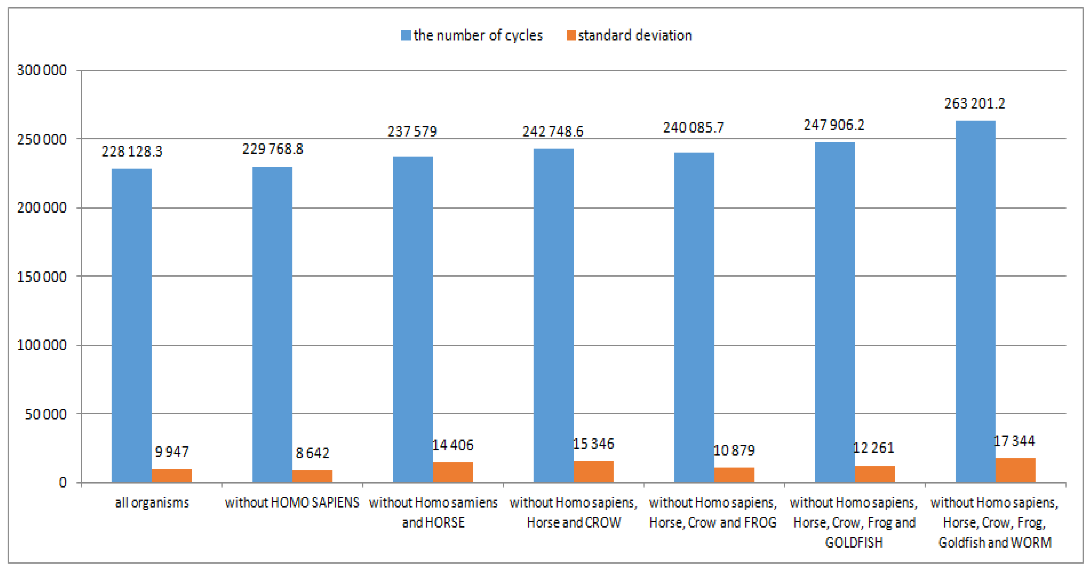
The average number of teaching cycles and standard deviations of the number of teaching cycles for processes of teaching the 5-layer neural networks are presented in Figure 2.
Figure 2 shows that the removal of consecutive organisms from a set of organisms used to teach the ANNs does not have a significant effect on the number of teaching cycles and standard deviations, although after removing the 6th organism, a slightly greater increase in these two values is visible, which can also indicate (and confirm) that this step (i.e., Worm recognition) should be the last step of the method.

3.6. Validation of the Method of Penetrating Deep into Evolution

In this section, is presented how the result of the method of penetrating deep into evolution can be validated. The reconstructed line of organism development was validated by 2-, 3-, 4- and 5-layer ANNs taught using 15 organisms and by phylogenetic tree generation. A set of birds (see Table A7 and Table A10 in Appendix A) and a set of amphibians and reptiles (see Table A8 and Table A11 in Appendix A) were used for the validation.

3.6.1. Validation of the Reconstructed Line of Organism Development by Determining Timestamps for a Set of Birds

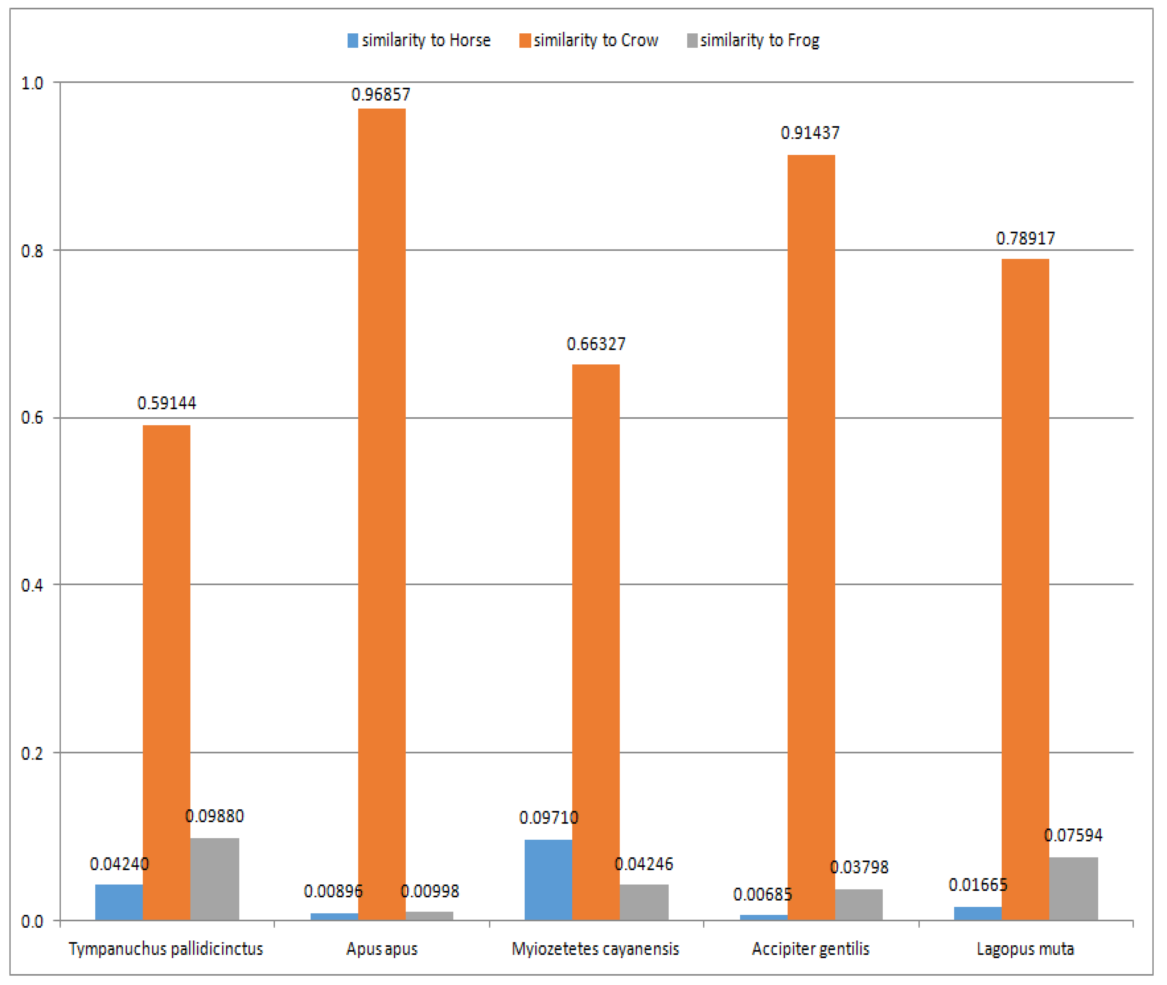
At the beginning, the reconstructed line of organism development was validated using a set of birds (see Table A7 and Table A10 in Appendix A). In Figure 3, the average similarities (calculated as the arithmetic means of similarities recognized by the 2-, 3-, 4- and 5-layer ANNs) for the three recognized largest outliers (i.e., Horse, Crow and Frog) are presented. The other outliers presented in Table A7 and Table A10 (see Appendix A) (i.e., Goldfish, Worm and Fly) are much smaller compared to Horse, Crow and Frog and, therefore, are not shown in Figure 3 for readability. As it can be seen, the similarities of each bird (from the set of birds used for validation) are the most obvious to Crow (see Table A7 in Appendix A). The background similarities to Horse and Frog are also visible (see Table A7 in Appendix A), which confirms the correctness of this part of the reconstructed line of organism development, i.e., birds are evolutionarily between Horse and Frog.

3.6.2. Validation of the Reconstructed Line of Organism Development by Determining Timestamps for a Set of Amphibians and Reptiles

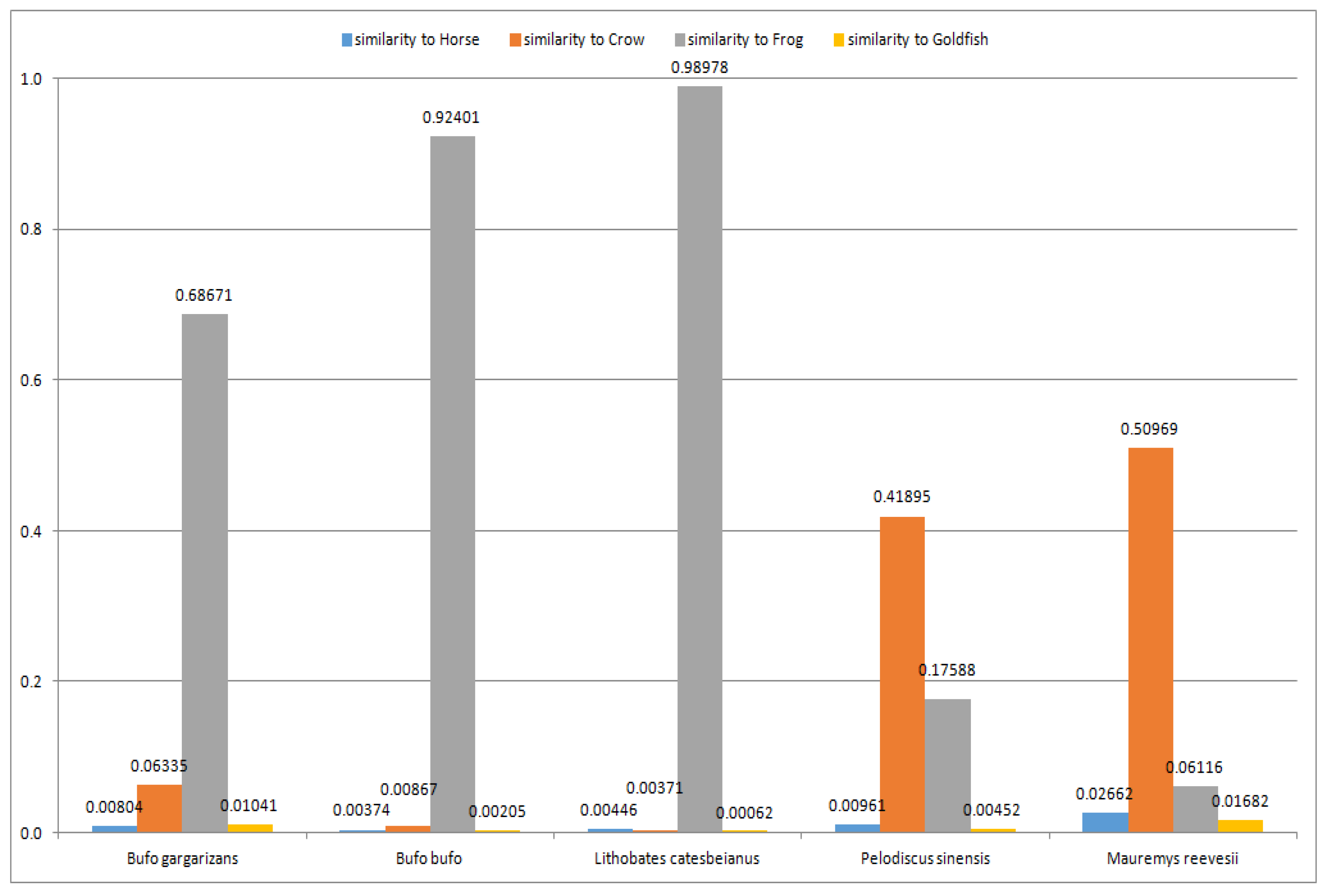
Next, the recognized line of organism evolution was validated using a set of amphibians (Bufo gargarizans, Bufo bufo and Lithobates catesbeianus) and reptiles (Pelodiscus sinensis and Mauremys reevesii) (see Table A8 and Table A11 in Appendix A). In Figure 4, the average similarities (calculated as the arithmetic means of similarities recognized by the 2-, 3-, 4- and 5-layer ANNs) for the four recognized largest outliers (i.e., Horse, Crow, Frog and Goldfish) are presented. The four largest outliers (out of the five outliers presented in Table A8 and Table A11 in Appendix A) are shown in Figure 4 to ensure readability.
As it can be seen, the similarities of each amphibian (from the set of amphibians used for validation) are the greatest to Frog (see Table A8 in Appendix A). The background similarities to Horse, Crow and Goldfish are also visible (see Table A8 in Appendix A), which confirms the correctness of this part of the reconstructed line of organism development, i.e., amphibians are evolutionarily between birds and fish (this conclusion is also supported by other works [44]). Moreover, it can be observed that reptiles (Pelodiscus sinensis and Mauremys reevesii) are evolutionarily between birds (Crow) and amphibians (Frog) (closer to Crow), which is in accordance with other authors [44].

3.6.3. Validation of the Reconstructed Line of Organism Development by Phylogenetic Tree Generation

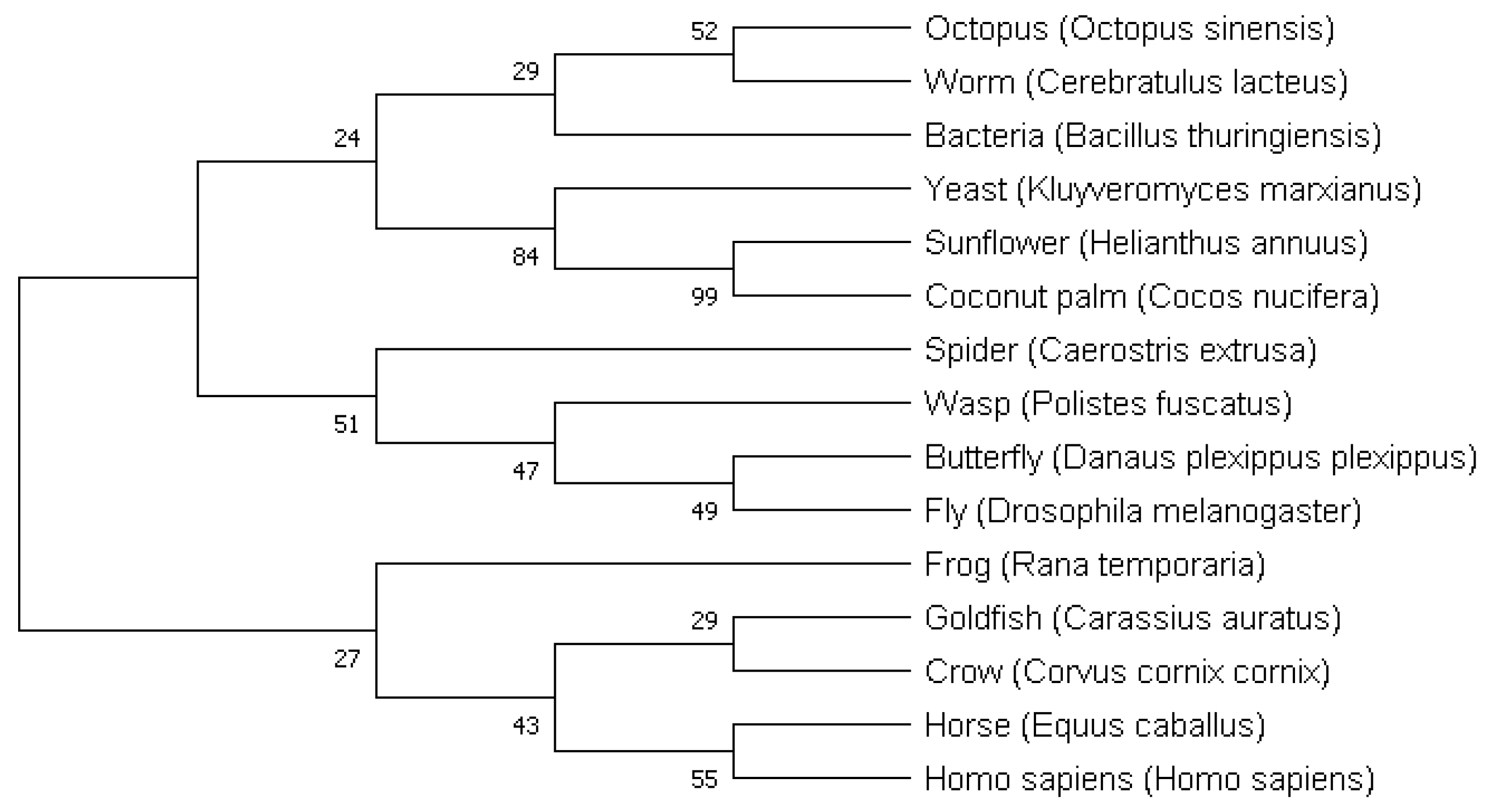
The reconstructed line of organism development was validated by phylogenetic tree generation. The trees were generated using the MEGA X program [29]. The phylogenetic trees were generated for 15 organisms used for ANN teaching using the Maximum Likelihood (ML) method with Poisson correction [45,46]. This method was used because it is considered one of the most accurate and widely used methods for reconstructing phylogenetic trees [46,47]. The ML method approaches a phylogenetic tree from a probabilistic point of view and looks for a tree that maximizes the probability of observing a given set of sequences on the tree leaves [46]. In this work, the bootstrap method with 1000 replications (Figure 5) and 10,000 replications (i.e., maximum number of replications in the MEGA X program) (Figure 6) was used to determine the reliability of the generated tree nodes. Trees were generated for different values of replications to check the effect of the number of replications on the reliability of the tree nodes.
Figure 5 and Figure 6 show that the increase in the number of replications has not significantly affected the reliability of the tree nodes. Although the reliability of the tree nodes (for both 1000 and 10,000 replications) can hardly be considered satisfactory (see the Introduction for a possible cause), it is apparent that the most and the least developed organisms are Homo sapiens and Bacteria, respectively. The closest organism to Homo sapiens is Horse (from the organisms used for ANN teaching), which confirms the results obtained using the method of penetrating deep into evolution. Moreover, the closest organisms to Worm are Octopus and Bacteria, which is in accordance with the last step of the method of penetrating deep into evolution. Additionally, evolutionary relationships between Worm and Octopus can be confirmed by the works of other authors [44,48]. In accordance with the generated tree, Goldfish is the closest to Crow, but the reliability of common node between these two organisms has a reliability of only 26% (for 1000 replications) and 29% (for 10,000 replications), so it is difficult to trust this result. The method of penetrating deep into evolution allowed the determination of a result that fits better with the modern theory of evolution, i.e., Frog (as a representative of amphibians) is the closest to Crow (as a representative of birds) considering the organisms used to teach the ANNs, which is in accordance with the results of other authors (for example, [23,44,49]).
The presented considerations show that the proposed method makes it possible to narrow down the area of considerations to the timestamp (i.e., set of recognized outliers) that was recognized in the each step of the algorithm (see the algorithm presented in the General Algorithm of Penetrating Deep Into Evolution Method and Reconstructing the Line of Organism Development Section). Travelling between genome attractors and narrowing down the area of considerations to the recognized timestamp (that contains only a small number of outliers comparing to the entire number of organisms) makes possible to obtain more reliable results compared to the reliability of the results obtained by generating phylogenetic trees. In the algorithms of phylogenetic tree generation (including the algorithms of the Neighbor Joining, Maximum Parsimony and Maximum Likelihood methods), the generated trees are evaluated on the basis of the evaluation of the trees as the whole, i.e., the generated trees are evaluated taking into account the entire sets of the nodes and branches [50]. This means that, although the generated tree will meet the assumed criteria as a whole, locally, it may contain internal nodes of lower reliabilities (and this is exactly what was obtained when generating the tree using the Maximum Likelihood method in this work; see Figure 5 and Figure 6). In accordance with the information presented in the Introduction, an important factor related to lower reliability of the nodes is the impossibility of evaluating all possible trees for more organisms. The number of possible rooted trees (calculated for n organisms as (2n − 3)!/(2n−2(s − 2)!)) for n = 15 (i.e., for the number of organisms considered in this article)) is equal to 213,458,046,676,875 [51]. The number of trees grows very quickly with the increase in the number of organisms and, for n = 50, the number of possible rooted trees is greater than the number of atoms in the universe [26]. This may indicate and also justify the need to narrow down the area of considerations in order to obtain a greater reliability when determining the course of evolution and reconstructing the line of organism development.

3.7. General Algorithm of the Method of Penetrating Deep into Evolution and Reconstructing the Line of Organism Development

In the light of the presented idea, the general algorithm of the method of penetrating deep into evolution and reconstructing the line of organism development is presented in the following steps:
Step 1.
Set the organisms in random order.
Step 2.
Teach the artificial neural network (ANN) using a full set of organisms.
Step 3.
Recognize the evolutionary timestamp (i.e., recognize a set of outliers) by recognizing the similarity to Homo sapiens using the ANN.
Step 4.
Add the organism represented by the biggest outlier to the list of organisms.
Step 5.
If the maximal number of iterations is archived or a sufficiently primitive organism to finish the algorithm is added to the list, stop the algorithm.
Step 6.
Remove the organism represented by the biggest outlier from the set of organisms.
Step 7.
Teach the ANN using the reduced set of organisms.
Step 8.
Recognize the evolutionary timestamp by recognizing the similarity to the removed organism using the ANN.
Step 9.
Go back to Step 4.
As a result of executing this algorithm for a set of organisms, the created list will contain organisms written in the order from the most developed to the most primitive organisms.

4. Conclusions

This work showed that one of the features of evolutionary timestamps (i.e., a set of outliers recognized by an artificial neural network) is their transparency, which allows not only to determine the closest evolutionary organism but also to determine more distant organisms. In this article, it is presented that this feature allows for penetration deep into evolution. As a result, a general algorithm of penetrating deep into evolution was established, which allows to reconstruct the line of organism development from the most advanced to the most primitive organisms. It was also shown the way in which this line can be validated using, among others, recognized timestamps. Five-layer ANNs were used to demonstrate the application of the method of penetrating deep into evolution, for which the recognized similarities to the closest evolutionary organism were the greatest, as was demonstrated during validation. The work also showed that not only the number of homologous comparisons and length of identity fragments are important in determining the evolutionary relationships between organisms, but also the distribution of similarities between sequences (i.e., distribution of amino acids in the compared sequences). It is possible that lines reconstructed using the proposed method can be considered as main lines of development (i.e., lines that omit “side tracks” of development); however, this conclusion needs to be carefully corroborated in following works. Finding a way to reconstruct the line of organism development can be considered a great scientific challenge, so further continuation of this work is planned to confirm the effectiveness of the proposed method.
Funding

This research received no external funding.

Data Availability Statement

The cytochrome c amino-acid sequences selected for this study are available at http://staff.uz.zgora.pl/akaspers/Pro/sequences.txt (accessed on 20 March 2023). The EvolutionXXI and dotPicker programs were written by the author and are freely available at http://staff.uz.zgora.pl/akaspers/Pro/pgms.zip (accessed on 20 March 2023). EvolutionXXI (written in Java using the Joone framework) contains an implemented neural network and was used in this work to recognize timestamps. The dotPicker program (written in C#) contains an implemented multidimensional semihomologous Dot-Matrix method and was used in this work to determine similarities between sequences at the codon level.

Conflicts of Interest

The author declares no conflict of interest.

Appendix A

Table A1. Outliers recognized by the 2-layer ANN during the recognition of selected monkeys.
1. Pan troglodytes2. Symphalangus syndactylus
Outliers recognized by ANNHomo sapiensHorseCrowOutliers recognized by ANNHomo sapiensHorseCrow
Recognized similarity0.997900.001610.00129Recognized similarity0.995830.003150.00170
Standard deviation0.000010.000030.00001Standard deviation0.000160.000100.00003
3. Papio anubis4. Theropithecus gelada
Recognized similarity0.983060.004660.00176Recognized similarity0.942510.018580.00292
Standard deviation0.001460.000420.00016Standard deviation0.009080.002090.00034
5. Piliocolobus tephrosceles6. Rhinopithecus bieti
Recognized similarity0.969900.002670.00084Recognized similarity0.980420.001890.00404
Standard deviation0.003430.000230.00008Standard deviation0.001460.000160.00031
7. Macaca nemestrina8. Cercocebus atys
Recognized similarity0.981280.002900.00258Recognized similarity0.983520.004850.00161
Standard deviation0.001650.000240.00011Standard deviation0.001710.000440.00012
9. Trachypithecus cristatus10. Chlorocebus aethiops
Recognized similarity0.986000.005030.00178Recognized similarity0.987170.005180.00183
Standard deviation0.000680.000260.00011Standard deviation0.000630.000200.00010
11. Papio hamadryas12. Brachyteles arachnoides
Recognized similarity0.981760.002910.00065Recognized similarity0.763130.016740.00455
Standard deviation0.001760.000200.00005Standard deviation0.014450.001890.00050
13. Aotus azarai14. Saimiri boliviensis boliviensis
Recognized similarity0.743360.016110.00435Recognized similarity0.763020.010650.00729
Standard deviation0.014390.001900.00045Standard deviation0.017200.000990.00095
15. Alouatta belzebul16. Alouatta seniculus
Recognized similarity0.758630.016760.00450Recognized similarity0.750750.016600.00442
Standard deviation0.014380.001700.00056Standard deviation0.013480.001500.00050
17. Sapajus apella18. Leontopithecus chrysomelas
Recognized similarity0.730790.015440.00428Recognized similarity0.724570.008940.00587
Standard deviation0.020570.001850.00056Standard deviation0.024050.001100.00093
Table A2. Outliers recognized by the 3-layer ANN during the recognition of selected monkeys.
1. Pan troglodytes2. Symphalangus syndactylus
Outliers recognized by ANNHomo sapiensHorseCrowOutliers recognized by ANNHomo sapiensHorseCrow
Recognized similarity0.998060.001250.00073Recognized similarity0.996600.002540.00098
Standard deviation0.000050.000090.00013Standard deviation0.000220.000290.00018
3. Papio anubis4. Theropithecus gelada
Recognized similarity0.989870.003590.00091Recognized similarity0.965000.016740.00202
Standard deviation0.001260.000430.00020Standard deviation0.006590.003740.00048
5. Piliocolobus tephrosceles6. Rhinopithecus bieti
Recognized similarity0.984110.002000.00044Recognized similarity0.987440.001530.00203
Standard deviation0.002900.000420.00016Standard deviation0.001890.000200.00045
7. Macaca nemestrina8. Cercocebus atys
Recognized similarity0.989710.002110.00135Recognized similarity0.990400.003270.00108
Standard deviation0.001560.000390.00017Standard deviation0.001100.000390.00013
9. Trachypithecus cristatus10. Chlorocebus aethiops
Recognized similarity0.991410.003740.00102Recognized similarity0.991570.003710.00105
Standard deviation0.000510.000340.00022Standard deviation0.000680.000200.00016
11. Papio hamadryas12. Brachyteles arachnoides
Recognized similarity0.987880.002210.00042Recognized similarity0.872100.012300.00248
Standard deviation0.001420.000250.00006Standard deviation0.014160.002320.00057
13. Aotus azarai14. Saimiri boliviensis boliviensis
Recognized similarity0.866020.012080.00250Recognized similarity0.858860.008630.00400
Standard deviation0.015440.002500.00062Standard deviation0.020890.001880.00102
15. Alouatta belzebul16. Alouatta seniculus
Recognized similarity0.869500.012120.00248Recognized similarity0.870930.012120.00243
Standard deviation0.014790.002440.00061Standard deviation0.016650.001820.00054
17. Sapajus apella18. Leontopithecus chrysomelas
Recognized similarity0.861630.011490.00249Recognized similarity0.836290.007820.00347
Standard deviation0.014420.002130.00068Standard deviation0.023950.001680.00112
Table A3. Outliers recognized by the 4-layer ANN during the recognition of selected monkeys.
1. Pan troglodytes2. Symphalangus syndactylus
Outliers recognized by ANNHomo sapiensHorseCrowOutliers recognized by ANNHomo sapiensHorseCrow
Recognized similarity0.998070.001380.00039Recognized similarity0.997350.002110.00042
Standard deviation0.000090.000140.00039Standard deviation0.000160.000200.00044
3. Papio anubis4. Theropithecus gelada
Recognized similarity0.995760.002730.00044Recognized similarity0.987340.008960.00061
Standard deviation0.000340.000550.00044Standard deviation0.003740.002940.00061
5. Piliocolobus tephrosceles6. Rhinopithecus bieti
Recognized similarity0.994900.001770.00034Recognized similarity0.994660.002240.00061
Standard deviation0.001420.000710.00033Standard deviation0.000450.000580.00063
7. Macaca nemestrina8. Cercocebus atys
Recognized similarity0.995170.002750.00063Recognized similarity0.995960.002460.00056
Standard deviation0.000410.000770.00066Standard deviation0.000440.000460.00053
9. Trachypithecus cristatus10. Chlorocebus aethiops
Recognized similarity0.995990.002720.00049Recognized similarity0.996010.002900.00050
Standard deviation0.000500.000470.00046Standard deviation0.000390.000420.00047
11. Papio hamadryas12. Brachyteles arachnoides
Recognized similarity0.994980.003210.00034Recognized similarity0.957530.018780.00136
Standard deviation0.000930.000600.00032Standard deviation0.014260.006580.00130
13. Aotus azarai14. Saimiri boliviensis boliviensis
Recognized similarity0.956900.017270.00131Recognized similarity0.949050.017810.00180
Standard deviation0.015140.005840.00118Standard deviation0.021730.008210.00175
15. Alouatta belzebul16. Alouatta seniculus
Recognized similarity0.957520.017680.00137Recognized similarity0.955830.018460.00134
Standard deviation0.015940.006640.00133Standard deviation0.015610.006900.00135
17. Sapajus apella18. Leontopithecus chrysomelas
Recognized similarity0.952830.019670.00135Recognized similarity0.944520.017060.00139
Standard deviation0.017090.007870.00125Standard deviation0.033480.010780.00128
Table A4. Outliers recognized by the 5-layer ANN during the recognition of selected monkeys.
1. Pan troglodytes2. Symphalangus syndactylus
Outliers recognized by ANNHomo sapiensHorseCrowOutliers recognized by ANNHomo sapiensHorseCrow
Recognized similarity0.998080.001250.00064Recognized similarity0.997820.001750.00058
Standard deviation0.000100.000190.00055Standard deviation0.000160.000320.00048
3. Papio anubis4. Theropithecus gelada
Recognized similarity0.997670.001750.00074Recognized similarity0.994350.005970.00060
Standard deviation0.000200.000290.00069Standard deviation0.002360.003180.00052
5. Piliocolobus tephrosceles6. Rhinopithecus bieti
Recognized similarity0.997380.001450.00109Recognized similarity0.997060.002090.00094
Standard deviation0.000650.000610.00121Standard deviation0.000850.000870.00087
7. Macaca nemestrina8. Cercocebus atys
Recognized similarity0.997230.002070.00111Recognized similarity0.997670.001670.00079
Standard deviation0.000580.000880.00124Standard deviation0.000180.000290.00074
9. Trachypithecus cristatus10. Chlorocebus aethiops
Recognized similarity0.997590.001890.00076Recognized similarity0.997650.001850.00076
Standard deviation0.000260.000390.00069Standard deviation0.000220.000340.00069
11. Papio hamadryas12. Brachyteles arachnoides
Recognized similarity0.997440.001900.00091Recognized similarity0.984980.014270.00136
Standard deviation0.000320.000730.00093Standard deviation0.009540.010310.00136
13. Aotus azarai14. Saimiri boliviensis boliviensis
Recognized similarity0.986170.013020.00129Recognized similarity0.970920.029900.00175
Standard deviation0.008410.008870.00124Standard deviation0.026180.029370.00175
15. Alouatta belzebul16. Alouatta seniculus
Recognized similarity0.986580.012810.00135Recognized similarity0.985010.013310.00139
Standard deviation0.007840.009570.00136Standard deviation0.010280.009630.00139
17. Sapajus apella18. Leontopithecus chrysomelas
Recognized similarity0.983820.014480.00137Recognized similarity0.959090.040330.00173
Standard deviation0.010600.009460.00137Standard deviation0.041690.040780.00170
Table A5. Outliers recognized by the 6-layer ANN during the recognition of selected monkeys.
1. Pan troglodytes2. Symphalangus syndactylus
Outliers recognized by ANNHomo sapiensHorseCrowOutliers recognized by ANNHomo sapiensHorseCrow
Recognized similarity0.997870.001370.00030Recognized similarity0.997770.00170.00035
Standard deviation0.000190.000410.00044Standard deviation0.000270.000610.00055
3. Papio anubis4. Theropithecus gelada
Recognized similarity0.997710.001650.0003Recognized similarity0.994130.005920.00074
Standard deviation0.00030.000520.00045Standard deviation0.005450.007580.0014
5. Piliocolobus tephrosceles6. Rhinopithecus bieti
Recognized similarity0.996190.001970.00018Recognized similarity0.996880.002430.00041
Standard deviation0.00220.001690.00023Standard deviation0.001660.001850.00069
7. Macaca nemestrina8. Cercocebus atys
Recognized similarity0.996930.002470.00033Recognized similarity0.997610.001810.00027
Standard deviation0.001160.001410.0005Standard deviation0.000370.00070.00038
9. Trachypithecus cristatus10. Chlorocebus aethiops
Recognized similarity0.997550.001930.00029Recognized similarity0.997590.001930.00029
Standard deviation0.000540.000810.00042Standard deviation0.000460.000770.00042
11. Papio hamadryas12. Brachyteles arachnoides
Recognized similarity0.997190.002240.00028Recognized similarity0.871770.14960.00053
Standard deviation0.001050.001310.00041Standard deviation0.234440.286750.0008
13. Aotus azarai14. Saimiri boliviensis boliviensis
Recognized similarity0.910120.111820.00048Recognized similarity0.827090.186390.00079
Standard deviation0.166540.239950.00074Standard deviation0.303160.336230.00127
15. Alouatta belzebul16. Alouatta seniculus
Recognized similarity0.898110.124390.0005Recognized similarity0.891140.125020.00051
Standard deviation0.18810.251930.00075Standard deviation0.213980.271960.00078
17. Sapajus apella18. Leontopithecus chrysomelas
Recognized similarity0.829680.165250.00055Recognized similarity0.770370.226130.00067
Standard deviation0.312040.312960.0008Standard deviation0.332520.335910.00102
Table A6. Outliers recognized by the ANNs during the recognition of selected fish.
Checked Organisms
Outliers Recognized by ANNsANN Type and SemihomologyEpinephelus moaraEpinephelus fuscoguttatusBrienomyrus brachyistiusHypomesus transpacificusNothobranchius furzeri
Horse2-layer0.000740.000340.000420.000210.00019
3-layer0.001000.000370.000280.000190.00013
4-layer0.044040.014810.006660.007070.00227
5-layer0.017650.007190.013030.007640.01524
[R/#/$/-][88/4/3/10][88/4/4/9][91/4/3/7][85/7/5/8][95/3/4/3]
Crow2-layer0.000710.000960.001390.002410.00038
3-layer0.000860.000940.001120.002530.00029
4-layer0.014660.013060.010280.023470.00505
5-layer0.069870.031820.049550.101260.02373
[R/#/$/-][89/6/4/6][90/5/4/6][93/4/4/4][87/5/5/8][98/4/3/0]
Frog2-layer0.035350.039590.010890.015080.04843
3-layer0.002700.002450.000570.000840.00211
4-layer0.000540.000880.000390.000220.00201
5-layer0.000530.001180.000890.000540.00458
[R/#/$/-][88/3/7/7][88/3/6/8][91/2/5/7][85/4/8/8][92/2/3/8]
Goldfish2-layer0.665740.697110.767560.642890.83611
3-layer0.337390.418240.599900.375400.57080
4-layer0.266690.376470.677010.364060.60185
5-layer0.877960.923570.941760.898730.88947
[R/#/$/-][96/4/2/2][97/3/2/2][97/3/4/0][91/4/4/5][91/6/3/5]
Worm2-layer0.000160.000160.000660.000260.00059
3-layer0.000260.000330.001330.000440.00146
4-layer0.000090.000140.000520.000210.00107
5-layer0.001280.001410.001510.001510.00260
[R/#/$/-][72/5/15/13][72/5/14/14][75/3/14/13][70/7/15/13][78/5/11/11]
Table A7. Outliers recognized by the ANNs during the recognition of selected birds.
Checked Organisms
Outliers Recognized by ANNsANN Type and SemihomologyTympanuchus pallidicinctusApus apusMyiozetetes cayanensisAccipiter gentilisLagopus muta
Horse2-layer0.035770.012000.098900.005950.01448
3-layer0.035130.009450.090470.005220.01283
4-layer0.020180.004930.040830.003740.00860
5-layer0.078520.009450.158180.012480.03070
[R/#/$/-][95/3/5/2][95/2/4/4][97/2/3/3][93/4/5/3][95/3/4/3]
Crow2-layer0.396970.943280.578730.835600.63272
3-layer0.534190.965960.672070.919170.75749
4-layer0.611470.977660.645980.952700.84513
5-layer0.823110.987380.756290.950010.92133
[R/#/$/-][97/4/4/0][101/2/1/1][99/2/2/2][98/5/2/0][98/4/3/0]
Frog2-layer0.034940.005420.008500.015130.03036
3-layer0.064800.009250.020440.023150.05228
4-layer0.159250.014770.063310.044200.10086
5-layer0.136220.010460.077600.069450.12024
[R/#/$/-][92/2/2/9][91/0/5/9][91/1/4/9][91/2/4/8][92/2/3/8]
Goldfish2-layer0.000190.000280.000080.000480.00030
3-layer0.000030.000120.000020.000100.00006
4-layer0.000020.000080.000010.000050.00003
5-layer0.004540.000540.000350.006140.00630
[R/#/$/-][90/6/4/5][91/4/4/6][90/4/4/7][90/7/3/5][91/6/3/5]
Worm2-layer0.001010.000840.001490.000830.00095
3-layer0.000570.000580.000720.000580.00061
4-layer0.000120.000220.000110.000260.00019
5-layer0.001420.000660.003720.000860.00095
[R/#/$/-][78/5/10/12][78/4/12/11][78/5/10/12][78/4/12/11][78/5/11/11]
Fly2-layer0.000010.000010.000010.000020.00001
3-layer0.000940.000690.000580.002030.00101
4-layer0.000200.000150.000190.000270.00017
5-layer0.000370.000290.000580.000290.00028
[R/#/$/-][10/15/22/58][10/14/23/58][10/14/24/57][10/15/22/58][10/15/22/58]
Table A8. Outliers recognized by the ANNs during the recognition of selected amphibians and reptiles.
Checked Organisms
Outliers Recognized by ANNsANN Type and SemihomologyBufo gargarizansBufo bufoLithobates catesbeianusPelodiscus sinensisMauremys reevesii
Horse2-layer0.007360.004450.005770.004650.03108
3-layer0.009450.004610.006540.004320.02970
4-layer0.006960.001870.004330.007950.01185
5-layer0.008390.004040.001210.021500.03386
[R/#/$/-][86/2/7/10][85/3/7/10][91/3/5/6][93/5/6/1][95/3/4/3]
Crow2-layer0.000670.000300.001010.189840.22497
3-layer0.000600.000240.000920.249760.32642
4-layer0.008580.001950.002020.375380.68809
5-layer0.243550.032200.010870.860800.79926
[R/#/$/-][86/1/7/11][85/2/7/11][92/1/6/6][96/3/6/0][96/2/6/1]
Frog2-layer0.648790.892230.987010.110960.02163
3-layer0.611770.889360.988490.123910.02753
4-layer0.692840.928090.992400.303600.05976
5-layer0.793440.986350.991230.165040.13571
[R/#/$/-][91/1/6/7][92/0/6/7][103/1/1/0][93/1/4/7][90/0/6/9]
Goldfish2-layer0.005490.002570.000650.000400.00091
3-layer0.000510.000160.000020.000050.00034
4-layer0.001920.001000.000150.000030.00036
5-layer0.033730.004480.001660.017610.06565
[R/#/$/-][86/1/4/14][85/2/4/14][91/3/5/6][90/5/5/5][92/4/3/6]
Worm2-layer0.000810.001670.000420.000710.00160
3-layer0.001220.002580.000440.000540.00135
4-layer0.001480.004270.000370.000140.00061
5-layer0.000970.005070.000520.001190.00081
[R/#/$/-][74/3/16/12][75/2/16/12][76/5/12/12][76/5/12/12][79/3/11/12]
Table A9. Standard deviation associated with the recognition of selected fish.
Checked Organisms
Outliers Recognized by ANNsANN TypeEpinephelus moaraEpinephelus fuscoguttatusBrienomyrus brachyistiusHypomesus transpacificusNothobranchius furzeri
Horse2-layer0.00010.000050.000050.000030.00002
3-layer0.000260.000090.000040.000050.00003
4-layer0.032440.013870.003830.007010.00173
5-layer0.041330.012130.023620.016080.04559
Crow2-layer0.000080.000110.000120.000330.00005
3-layer0.000310.000270.000310.000880.00006
4-layer0.014930.011160.010270.016550.00912
5-layer0.114070.034470.06650.174580.03659
Frog2-layer0.003770.003670.001220.001720.00557
3-layer0.002750.002490.000570.000730.00207
4-layer0.000970.002130.000990.000310.00564
5-layer0.000980.002730.001640.000980.00761
Goldfish2-layer0.01640.01590.016390.032490.01223
3-layer0.065390.069570.068810.061660.06064
4-layer0.231760.205220.161850.210310.17467
5-layer0.130770.095760.061070.163560.17743
Worm2-layer0.000030.000030.000110.000060.0001
3-layer0.000080.000120.000340.000110.00033
4-layer0.000080.000110.000320.000130.00051
5-layer0.003810.003860.00390.004390.0048
Table A10. Standard deviation associated with the recognition of selected birds.
Checked Organisms
Outliers Recognized by ANNsANN TypeTympanuchus pallidicinctusApus apusMyiozetetes cayanensisAccipiter gentilisLagopus muta
Horse2-layer0.002990.000790.008410.000630.00124
3-layer0.007540.001990.020250.001680.00288
4-layer0.008290.001690.013350.002650.00422
5-layer0.145060.018270.266260.024230.06237
Crow2-layer0.019080.003030.019780.012820.01667
3-layer0.060040.004950.054820.018720.03813
4-layer0.162090.010110.189760.033460.06475
5-layer0.235610.010820.272440.046770.10369
Frog2-layer0.002630.000430.000650.001250.00260
3-layer0.013150.002300.006080.004630.00924
4-layer0.081090.007570.040270.032900.04887
5-layer0.286080.012260.213760.086210.23742
Goldfish2-layer0.000010.000020.000010.000050.00002
3-layer0.000010.000020.000010.000030.00002
4-layer0.000030.000060.000010.000080.00007
5-layer0.013440.000930.000710.018420.01890
Worm2-layer0.000170.000090.000210.000120.00014
3-layer0.000210.000250.000270.000260.00023
4-layer0.000090.000110.000130.000180.00012
5-layer0.002440.001140.00790.001910.00161
Fly2-layer0.000000.000000.000000.000010.00000
3-layer0.000360.000190.000190.000710.00038
4-layer0.000280.000190.000320.000280.00019
5-layer0.001160.000910.001830.000920.00088
Table A11. Standard deviation associated with the recognition of selected amphibians and reptiles.
Checked Organisms
Outliers Recognized by ANNsANN TypeBufo gargarizansBufo bufoLithobates catesbeianusPelodiscus sinensisMauremys reevesii
Horse2-layer0.001150.000530.000380.000640.00387
3-layer0.004250.001990.000380.001060.00739
4-layer0.004990.001300.003330.005360.0063
5-layer0.016950.008510.002060.040380.07599
Crow2-layer0.000120.000050.000050.017370.01585
3-layer0.000310.000100.000150.049860.04298
4-layer0.021210.004540.001560.147710.09737
5-layer0.366940.051800.014710.181950.25729
Frog2-layer0.037220.015250.00090.007660.00167
3-layer0.085950.031210.001610.0210.00703
4-layer0.154680.038520.00190.15720.03855
5-layer0.180750.010.008020.284880.18174
Goldfish2-layer0.000590.000270.00010.000050.00009
3-layer0.000420.000140.000020.000020.00011
4-layer0.005580.003040.000470.000090.00066
5-layer0.06710.00910.003010.054820.2018
Worm2-layer0.00010.000190.000030.000110.00018
3-layer0.000280.00060.000040.000180.00038
4-layer0.000510.001490.000160.000130.00036
5-layer0.000950.006530.000180.001420.00108

References

  1. Mazzocca, A. The Systemic–Evolutionary Theory of the Origin of Cancer (SETOC): A New Interpretative Model of Cancer as a Complex Biological System. Int. J. Mol. Sci. 2019, 20, 4885. [Google Scholar] [CrossRef] [PubMed]
  2. Kováč, L. Lamarck and Darwin revisited. EMBO Rep. 2019, 20, 47922. [Google Scholar] [CrossRef] [PubMed]
  3. Kasperski, A. Life Entrapped in a Network of Atavistic Attractors: How to Find a Rescue. Int. J. Mol. Sci. 2022, 23, 4017. [Google Scholar] [CrossRef] [PubMed]
  4. Kasperski, A.; Kasperska, R. Study on attractors during organism evolution. Sci. Rep. 2021, 11, 9637. [Google Scholar] [CrossRef]
  5. Kasperski, A. Genome Attractors as Places of Evolution and Oases of Life. Processes 2021, 9, 1646. [Google Scholar] [CrossRef]
  6. Kasperski, A.; Kasperska, R. A new approach to the automatic identification of organism evolution using neural networks. Biosystems 2016, 142–143, 32–42. [Google Scholar] [CrossRef]
  7. Kasperski, A.; Kasperska, R. Application of n-dimensional dot-matrix to analysis of plant genetic diversity. Biul. IHAR 2015, 276, 69–83. [Google Scholar] [CrossRef]
  8. Kasperski, A.; Kasperska, R. Identifcation of protein family representatives. Curr. Bioinform. 2014, 9, 414–425. [Google Scholar] [CrossRef]
  9. Kasperski, A.; Kasperska, R. A novel method of sequence similarity evaluation in n-dimensional sequence space. Curr. Bioinform. 2012, 7, 295–303. [Google Scholar] [CrossRef]
  10. Kasperski, A. Modelling of Cells Bioenergetics. Acta Biotheor. 2008, 56, 233–247. [Google Scholar] [CrossRef]
  11. Kasperski, A.; Kasperska, R. Bioenergetics of life, disease and death phenomena. Theory Biosci. 2018, 137, 155–168. [Google Scholar] [CrossRef]
  12. Kasperski, A.; Kasperska, R. Selected disease fundamentals based on the unified cell bioenergetics. J. Investig. Biochem. 2013, 2, 93–100. [Google Scholar] [CrossRef]
  13. Kasperski, A.; Miśkiewicz, T. Optimization of pulsed feeding in a Baker’s yeast process with dissolved oxygen concentration as a control parameter. Biochem. Eng. J. 2008, 40, 321–327. [Google Scholar] [CrossRef]
  14. Kasperski, A.; Miśkiewicz, T. An adaptive fuzzy logic controller using the respiratory quotient as an indicator of overdosage in the baker’s yeast process. Biotechnol. Lett. 2002, 24, 17–21. [Google Scholar] [CrossRef]
  15. Miśkiewicz, T.; Kasperski, A. A fuzzy logic controller to control nutrient dosage in a fed-batch baker’s yeast process. Biotechnol. Lett. 2000, 22, 1685–1691. [Google Scholar] [CrossRef]
  16. Damasco, A.; Giuliani, A. A resonance based model of biological evolution. Phys. A Stat. Mech. Its Appl. 2017, 471, 750–756. [Google Scholar] [CrossRef]
  17. Harvey, P.H.; Pagel, M.D. The Comparative Method in Evolutionary Biology; Oxford University Press: Oxford, UK, 1991; Volume 239. [Google Scholar]
  18. Lewin, R. Complexity: Life at the Edge of Chaos; Collier Books: Springfield, OH, USA, 1993. [Google Scholar]
  19. Giuliani, A. Review of Thomas McCabe (ed.) 2021, Descente and Logic in Biosystematics. Juneau: Perseverant Publishing. Org. J. Biol. Sci. 2021, 5, 87–88. [Google Scholar]
  20. Keya, K.; Priya, S. A Study of Phylogenetic Relationships and Homology of Cytochrome C Using Bioinformatics. Int. Res. J. Sci. Eng. 2016, 4, 65–75. [Google Scholar]
  21. Kumar, S. Molecular clocks: Four decades of evolution. Nat. Rev. Genet. 2005, 6, 654–662. [Google Scholar] [CrossRef]
  22. Margoliash, E. Primary Structure and Evolution of Cytochrome C. Proc. Natl. Acad. Sci. USA 1963, 50, 672–679. [Google Scholar] [CrossRef]
  23. Gregory, T.R. Understanding Evolutionary Trees. Evo. Edu. Outreach. 2008, 1, 121–137. [Google Scholar] [CrossRef]
  24. Hodkinson, T.R.; Parnell, J.A.N. (Eds.) Reconstructing the Tree of Life: Taxonomy and Systematics of Species Rich Taxa; CRC Press: Boca Raton, FL, USA, 2019. [Google Scholar]
  25. Lecointre, G.; Le Guyader, H. The Tree of Life: A Phylogenetic Classification; Belknap: Cambridge, MA, USA, 2007. [Google Scholar]
  26. Hall, B.G. Phylogenetic Trees Made Easy; Oxford University Press Inc.: New York, NY, USA, 2017. [Google Scholar]
  27. Felsenstein, J. Confidence limits on phylogenies: An approach using the bootstrap. Evolution 1985, 39, 783–791. [Google Scholar] [CrossRef] [PubMed]
  28. Efron, B. The Jackknife, the Bootstrap and Other Resampling Plans; CBMS-NSF Regional Conference Series in Applied Mathematics, Monograph 38; SIAM: Philadelphia, PA, USA, 1982. [Google Scholar]
  29. Kumar, S.; Stecher, G.; Li, M.; Knyaz, C.; Tamura, K. MEGA X: Molecular Evolutionary Genetics Analysis across Computing Platforms. Mol. Biol. Evol. 2018, 35, 1547–1549. [Google Scholar] [CrossRef] [PubMed]
  30. Karthikeyan, A.; Priyakumar, U.D. Artificial intelligence: Machine learning for chemical sciences. J. Chem. Sci. 2022, 134, 2. [Google Scholar] [CrossRef] [PubMed]
  31. O’connell, G.C.; Walsh, K.B.; Smothers, C.G.; Ruksakulpiwat, S.; Armentrout, B.L.; Winkelman, C.; Milling, T.J.; Warach, S.J.; Barr, T.L. Use of deep artificial neural networks to identify stroke during triage via subtle changes in circulating cell counts. BMC Neurol. 2022, 22, 206. [Google Scholar] [CrossRef]
  32. Niazkar, H.R.; Niazkar, M. Application of artificial neural networks to predict the COVID-19 outbreak. Glob. Health Res. Policy 2020, 5, 50. [Google Scholar] [CrossRef]
  33. Topczewska, J.; Kwater, T. Forecasting the Utility Value of Hucul Horses by Means of Artificial Intelligence. Sustainability 2020, 12, 7989. [Google Scholar] [CrossRef]
  34. Qian, N.; Sejnowski, T.J. Predicting the secondary structure of globular proteins using neural network models. J. Mol. Biol. 1988, 202, 865–884. [Google Scholar] [CrossRef]
  35. Graupe, D. Principles of Artificial Neural Networks, 3rd ed.; World Scientific: Singapore, 2013. [Google Scholar]
  36. Krogh, A. What are artificial neural networks? Nat. Biotechnol. 2008, 26, 195–197. [Google Scholar] [CrossRef]
  37. Han, S.-H.; Kim, K.W.; Kim, S.; Youn, Y.C. Artificial Neural Network: Understanding the Basic Concepts without Mathematics. Dement. Neurocognitive Disord. 2018, 17, 83–89. [Google Scholar] [CrossRef]
  38. Rashid, T.; Huang, B.Q.; Kechadi, M.T. A new simple recurrent network with real-time recurrent learning process. In Proceedings of the 14th Irish Conference on Artificial Intelligence & Cognitive Science, AICS 2003, Dublin, Ireland, 17–19 September 2003; pp. 169–174. [Google Scholar]
  39. Menon, A.; Mehrotra, K.; Mohan, C.K.; Ranka, S. Characterization of a Class of Sigmoid Functions with Applications to Neural Networks. Neural Netw. 1996, 9, 819–835. [Google Scholar] [CrossRef] [PubMed]
  40. Masters, T. Practical Neural Network Recipes in C++; Academic Press: San Diego, CA, USA, 1993. [Google Scholar]
  41. Leluk, J. A non-statistical approach to protein mutational variability. Biosystems 2000, 56, 83–93. [Google Scholar] [CrossRef]
  42. Leluk, J. Regularities in mutational variability in selected protein families and the Markovian model of amino acid replacement. Comput. Chem. 2000, 24, 659–672. [Google Scholar] [CrossRef] [PubMed]
  43. Leluk, J.; Konieczny, L.; Roterman, I. Search for structural similarity in proteins. Bioinformatics 2003, 19, 117–124. [Google Scholar] [CrossRef] [PubMed]
  44. Schnell, A.K.; Amodio, P.; Boeckle, M.; Clayton, N.S. How intelligent is a cephalopod? Lessons from comparative cognition. Biol. Rev. 2021, 96, 162–178. [Google Scholar] [CrossRef]
  45. Dhar, A.; Minin, V.N. Maximum Likelihood Phylogenetic Inference. In Encyclopedia of Evolutionary Biology; Kliman, R.M., Ed.; Academic Press: Cambridge, MA, USA, 2016; pp. 499–506. [Google Scholar]
  46. Jin, G.; Nakhleh, L.; Snir, S.; Tuller, T. Maximum likelihood of phylogenetic networks. Bioinformatics 2006, 22, 2604–2611. [Google Scholar] [CrossRef]
  47. Felsenstein, J. Evolutionary trees from DNA sequences: A maximum likelihood approach. J. Mol. Evol. 1981, 17, 368–376. [Google Scholar] [CrossRef]
  48. Vinogradov, A.E.; Anatskaya, O.V. Gradistics: An underappreciated dimension in evolutionary space. Biosystems 2023, 224, 104844. [Google Scholar] [CrossRef]
  49. Nassar, L.R.; Barber, G.P.; Benet-Pagès, A.; Casper, J.; Clawson, H.; Diekhans, M.; Fischer, C.; Gonzalez, J.N.; Hinrichs, A.S.; Lee, B.T.; et al. The UCSC Genome Browser database: 2023 update. Nucleic Acids Res. 2022, 51, D1188–D1195. [Google Scholar] [CrossRef]
  50. Goldstein, D. Indo-European phylogenetics with R. Indo-Eur. Linguist. 2020, 8, 110–180. [Google Scholar] [CrossRef]
  51. Felsenstein, J. The Number of Evolutionary Trees. Syst. Zool. 1978, 27, 27–33. [Google Scholar] [CrossRef]
Figure 1. The average number of teaching cycles and standard deviations for processes of teaching the neural networks.
Processes 11 01316 g001
Figure 2. The average number of teaching cycles and standard deviations for processes of teaching the 5-layer neural networks.
Processes 11 01316 g002
Figure 3. Validation of the reconstructed line of organism development using a set of birds. The recognized timestamps (i.e., sets of recognized outliers) indicate that birds are evolutionarily between Horse and Frog.
Processes 11 01316 g003
Figure 4. Validation of the reconstructed line of organism development using a set of amphibians (Bufo gargarizans, Bufo bufo and Lithobates catesbeianus) and reptiles (Pelodiscus sinensis and Mauremys reevesii). The recognized timestamps (i.e., sets of recognized outliers) indicate that amphibians are evolutionarily between Crow and Goldfish.
Processes 11 01316 g004
Figure 5. The generated bootstrap consensus tree with 1000 replications for the organisms used for ANN teaching.
Processes 11 01316 g005
Figure 6. The generated bootstrap consensus tree with 10,000 replications for the organisms used for ANN teaching.
Processes 11 01316 g006
Table 1. The set of organisms, listed in alphabetical order, used to teach the ANNs.
No.OrganismDescription of Sequence (First Line of the FASTA Format)
1Bacteria>PEK86573.1 cytochrome C [Bacillus thuringiensis]
2Butterfly>XP_032519089.1 cytochrome c [Danaus plexippus plexippus]
3Coconut palm>KAG1363645.1 Cytochrome c [Cocos nucifera]
4Crow>XP_039405800.1 cytochrome c [Corvus cornix cornix]
5Fly>AAA28437.1 cytochrome C [Drosophila melanogaster]
6Frog>XP_040208820.1 cytochrome c [Rana temporaria]
7Goldfish>XP_026069975.1 cytochrome c [Carassius auratus]
8Homo sapiens>NP_061820.1 cytochrome c [Homo sapiens]
9Horse>NP_001157486.1 cytochrome c [Equus caballus]
10Octopus>XP_029642027.1 cytochrome c [Octopus sinensis]
11Spider>GIY91737.1 cytochrome c [Caerostris extrusa]
12Sunflower>AAR30955.1 cytochrome c [Helianthus annuus]
13Wasp>XP_043491202.1 cytochrome c [Polistes fuscatus]
14Worm>AKI85307.1 cytochrome c [Cerebratulus lacteus]
15Yeast>BAP71068.1 cytochrome c [Kluyveromyces marxianus]
Table 2. The number of neurons in the layers of the implemented neural networks for the 15 organisms used for teaching.
ANN TypesNumber of Neurons in the Layers
2-layers (i.e., 0 hidden layers)525, 15
3-layers (i.e., 1 hidden layers)525, 89, 15
4-layers (i.e., 2 hidden layers)525, 160, 49, 15
5-layers (i.e., 3 hidden layers)525, 216, 89, 36, 15
6-layers (i.e., 4 hidden layers)525, 258, 127, 62, 31, 15
7-layers (i.e., 5 hidden layers)525, 290, 160, 89, 49, 27, 15
8-layers (i.e., 6 hidden layers)525, 316, 190, 114, 69, 41, 25, 15
Table 3. Timestamp (i.e., a set of recognized outliers) recognized by ANN during the recognition of Homo sapiens.
Outliers Recognized by ANNHomo Sapiens
Recognized similarity0.99808
Standard deviation0.00010
Table 4. Timestamp (i.e., a set of recognized outliers) recognized by ANN during the recognition of Homo sapiens after removing Homo sapiens from the set of organisms and re-teaching the network using the remaining organisms.
Outliers Recognized by ANNHorseCrowFrog
Recognized similarity0.972020.026930.00619
Standard deviation0.053200.045860.01771
Table 5. Timestamp recognized by ANN during the recognition of Horse after removing Homo sapiens and Horse from the set of organisms and re-teaching the network using the remaining organisms.
Outliers Recognized by ANNCrowFrogGoldfish
Recognized similarity0.909360.013220.04507
Standard deviation0.073370.014830.04704
Table 6. Timestamp recognized by ANN during the recognition of Crow after removing Homo sapiens, Horse and Crow from the set of organisms and re-teaching the network using the remaining organisms.
Outliers Recognized by ANNFrogGoldfish
Recognized similarity0.572320.49903
Standard deviation0.306610.31334
Table 7. Timestamp recognized by ANN during the recognition of Frog after removing Homo sapiens, Horse, Crow and Frog from the set of organisms and re-teaching the network using the remaining organisms.
Outliers Recognized by ANNGoldfishWorm
Recognized similarity0.934240.04564
Standard deviation0.111080.05963
Table 8. Timestamp recognized by ANN during the recognition of Goldfish after removing Homo sapiens, Horse, Crow, Frog and Goldfish from the set of organisms and re-teaching the network using the remaining organisms.
Outliers Recognized by ANNWorm
Recognized similarity0.99733
Standard deviation0.00038
Table 9. Timestamp recognized by ANN during the recognition of Worm after removing Homo sapiens, Horse, Crow, Frog, Goldfish and Worm from the set of organisms and re-teaching the network using the remaining organisms.
Outliers Recognized by ANNButterflySunflowerOctopusBacteria
Recognized similarity0.002390.061560.104060.52457
Standard deviation0.004380.136160.273360.42770
Table 10. Results of using semohomology approach to check the evolutionary distances between Worm and the organisms used to teach ANN in the last step of the method. The organisms in the table are listed in alphabetical order.
Organisms[R/#/$/-]
Bacteria[10/10/27/58]
Butterfly[11/11/25/59]
Coconut[4/13/31/58]
Fly[10/14/26/56]
Octopus[10/8/28/60]
Spider[8/11/31/55]
Sunflower[6/10/33/57]
Wasp[9/14/24/59]
Yeast[9/11/31/55]
Table 11. The number of neurons in the layers of the implemented 5-layer neural networks for the 15, 14, 13, 12, 11, 10 and 9 organisms used for teaching.
Number of Organisms Used for TeachNumber of Neurons in the Layers
15all organisms from the initial set of organisms525, 216, 89, 36, 15
14without Homo sapiens525, 212, 86, 35, 14
13without Homo sapiens and Horse525, 208, 83, 33, 13
12without Homo sapiens, Horse and Crow525, 204, 79, 31, 12
11without Homo sapiens, Horse, Crow and Frog 525, 200, 76, 29, 11
10without Homo sapiens, Horse, Crow, Frog and Goldfish525, 195, 72, 27, 10
9without Homo sapiens, Horse, Crow, Frog, Goldfish and Worm525, 190, 69, 25, 9
Disclaimer/Publisher’s Note: The statements, opinions and data contained in all publications are solely those of the individual author(s) and contributor(s) and not of MDPI and/or the editor(s). MDPI and/or the editor(s) disclaim responsibility for any injury to people or property resulting from any ideas, methods, instructions or products referred to in the content.