Article

Simulating Tablet Dissolution Using Computational Fluid Dynamics and Experimental Modeling

1
School of Chemical and Biomolecular Engineering, University of Sydney, Camperdown, NSW 2006, Australia
2
Drying and Process Technology Research Group, School of Chemical and Biomolecular Engineering, University of Sydney, Camperdown, NSW 2006, Australia
*
Author to whom correspondence should be addressed.
Processes 2023, 11(2), 505; https://doi.org/10.3390/pr11020505
Submission received: 13 January 2023 / Revised: 3 February 2023 / Accepted: 4 February 2023 / Published: 7 February 2023

Abstract

:
The study of mass transfer is essential in the food digestion process, especially when gastric acid interacts with food and nutrients dissolve in the gastric system. In this study, a computational fluid dynamics (CFD) model was built based on an in vitro study, which investigated the mass transfer in a tablet dissolution process in a beaker and stirrer system. The predicted mass transfer coefficients from the simulation aligned well with the experimental values. The effect of the type and rotation speed of the stirrers was also investigated. Mass transfer from the tablet was found to be closely related to the tablet Reynolds number of the fluid (ranging from 0 to 938) and the shear stress (0 to 0.167 Pa) acting on the tablet. The relationship between the power number (0.0061 to 0.196) and the Reynolds number for the impeller (719 to 5715) was also derived for different stirrers.

1. Introduction

It is relevant to compare food digestion and tablet dissolution behaviors, where the former is traditionally studied in food engineering and the latter in the pharmaceutical industry, because the complexity of the drug mixtures in some tablets can approach the variety of nutrients in some foods, both of which may travel through the gastrointestinal tract. The aims of the US Pharmacopeia [1] regarding the specification of a dissolution test apparatus may be closely aligned with the aims of food engineers who are trying to simulate stomach digestion systems through in-vitro testing apparatus, as reviewed by Li et al. [2] and Zhong and Langrish [3]. The aims of the US Pharmacopeia [1] in this field may be expressed as testing the release rates of pharmaceutical drugs from tablets or capsules in a standardized environment that is close (in some sense) to the human digestion process. Both the food industry [2,3] and the pharmaceutical industry [4,5] have strong interests in developing correlations between in vitro and in vivo dissolution, digestion and uptake data.
According to the US Pharmacopeia [1], there are four different recognized types of standard dissolution testing apparatus, as follows:
  • US Pharmacopoeia dissolution apparatus 1: basket apparatus; a wire mesh basket containing a tablet is rotated in a stationary fluid (largely superseded by apparatuses 2–4);
  • US Pharmacopoeia dissolution apparatus 2: paddle apparatus; a tablet freely moves in the bottom of a rounded-bottom flask with a rotating paddle stirrer;
  • US Pharmacopoeia dissolution apparatus 3: reciprocating cylinder; and
  • US Pharmacopoeia dissolution apparatus 4: flow through cell; a tablet fixed in the middle of a column where fluid flows up the column and around the tablet.
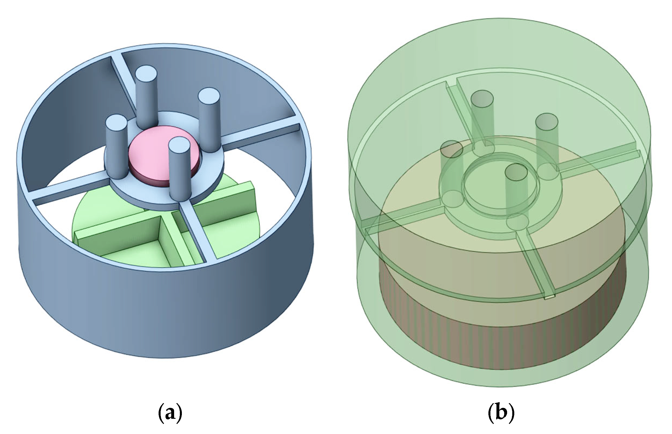
By contrast, in the area of food engineering, Zhong and Langrish [3] and Li et al. [2] reviewed 19 in-vitro digestion systems and nine systems, respectively.
Most of the above-described pieces of pharmaceutical dissolution apparatus have clear parallels in the food engineering field, as follows:
(a)
US Pharmacopoeia dissolution apparatus 2: paddle apparatus: similar to Kong and Singh [6], SHIME [7,8,9,10];
(b)
US Pharmacopoeia dissolution apparatus 3: reciprocating cylinder: similar to Chen et al. [11], Do et al. [12], Guerra et al. [13]; and
(c)
US Pharmacopoeia dissolution apparatus 4: flow through cell: similar to Passannanti et al. [14].
Although these types of US Pharmacopoeia dissolution apparatus are simple and standardized, which are key characteristics of the pharmaceutical industry, the amount of variability in fundamental parameters that govern mass transfer, dissolution and digestion may be very large, and the flow fields and flow patterns may be different to those in the human digestion system. Examples of fundamental parameters that govern mass transfer, dissolution and digestion are the shear stresses and shear strain rates in the fluid and around the tablets, where these stresses and strain rates vary widely, particularly in the paddle apparatus (USP dissolution apparatus 2 [15]). Detailed studies of the predicted flow fields (using CFD in some cases supported with experiments) in the USP dissolution apparatus 2 reveal the numerical ranges for shear strain rates: up to 60 s−1 (50–100 rpm [16]); 50–100 s−1 for a paddle stirrer speed of 50 rpm and 70–175 s−1 at 100 rpm [17]; up to 120 s−1 with different impeller locations, 50 rpm paddle speed [18]; up to 60 s−1 at 50 rpm [19]; and up to 36 s−1 at 50 rpm and up to 73 s−1 at 100 rpm [20].
There are several reasons why these shear strain rates (and induced shear stresses) are important. First, the shear stresses are very likely to be related to the external mass-transfer coefficients, through analogies between heat, mass, and momentum transfer, with the consequence that any differences between these strain rates (in the USP dissolution apparatus 2) and those in real stomachs are likely to have significant effects on differences in the external mass-transfer coefficients. Second, following this consideration, the shear stresses and shear strain rates in real stomach systems are typically over one order of magnitude greater than those in stirred systems (Table 6 in Zhong and Langrish [3]), including those in the USP dissolution apparatus 2.
The mass-transfer rates for the USP 2 dissolution apparatus (paddle) were measured by D’Arcy et al. [21] both experimentally and numerically. However, as the saturation concentration is dependent on the temperature, the mass-transfer rate also varies (implicitly) with the temperature. Compared with the mass-transfer rates, the mass-transfer coefficients are more fundamental parameters, but they were not measured in the study.
D’Arcy et al. [22] studied the USP 1 dissolution apparatus (basket) through an experiment by evaluating the dissolution rates of benzoic acid and salicylic acid tablets. However, the corresponding mass-transfer coefficients were not estimated or compared with other types of dissolution apparatus.
The hydrodynamics of the USP 4 dissolution apparatus (flow through cell) were investigated numerically by D’Arcy et al. [4], assuming the flow to be laminar and time-dependent. The dissolution rates of the benzoic acid and salicylic acid tablets were measured experimentally. In this study, the mass-transfer coefficients were not calculated either. In addition, no shear stresses or shear strain rates were estimated or measured. Once again, the results were not compared with other types of apparatus either.
An important gap in the above studies, both CFD analyses and experimental studies, is that the shear stresses directly above the tablets have not been simulated, and in the case of the common USP Apparatus 2 (paddle stirrer), the tablet has been free to move into different flow regions where the shear stresses vary widely. Mass transfer processes were also not simulated directly.
The remainder of this paper is organized as follows: Section 2 presents a summary of the experimental setup that is modelled in this paper, Section 3 contains a description of the CFD model, Section 4 contains the results and discussion and finally Section 5 contains the conclusions.

2. Experimental Study

Experimental Method and Procedure

The experimental method and procedure have been described in detail by Langrish et al. [23] and are summarized here. Briefly, a 13 mm diameter, 2.5 mm high tablet was pressed from benzoic acid (laboratory grade from Honeywell Fluka™) powder using a tableting press at a compression pressure of 111 MPa. The tablets were placed on a platform (Figure 1 in Langrish et al. [23]) 25 mm above the bottom of a 150 mL beaker containing either 80 mL or 120 mL of deionized water. Three types of stirrers were used, as shown in Figure 1, at rotational speeds of 0 rpm, 100 rpm, and 200 rpm. The concentration of benzoic acid in the bulk solution was monitored as a function of time with a Cary-60 UV-Visible spectrophotometer. Each experiment was repeated at least twice.
The concept behind the platform was to ensure that the tablet was fixed in place and did not move, since such movement is known [17] to cause significant variability in the dissolution behavior, due to the tablets being exposed to a wide range of different flow conditions (velocities and turbulence levels). The results of these experiments have been reported, together with an experimental error analysis and analysis of variance, in Langrish et al. [23].

3. Computational Fluid Dynamics Model
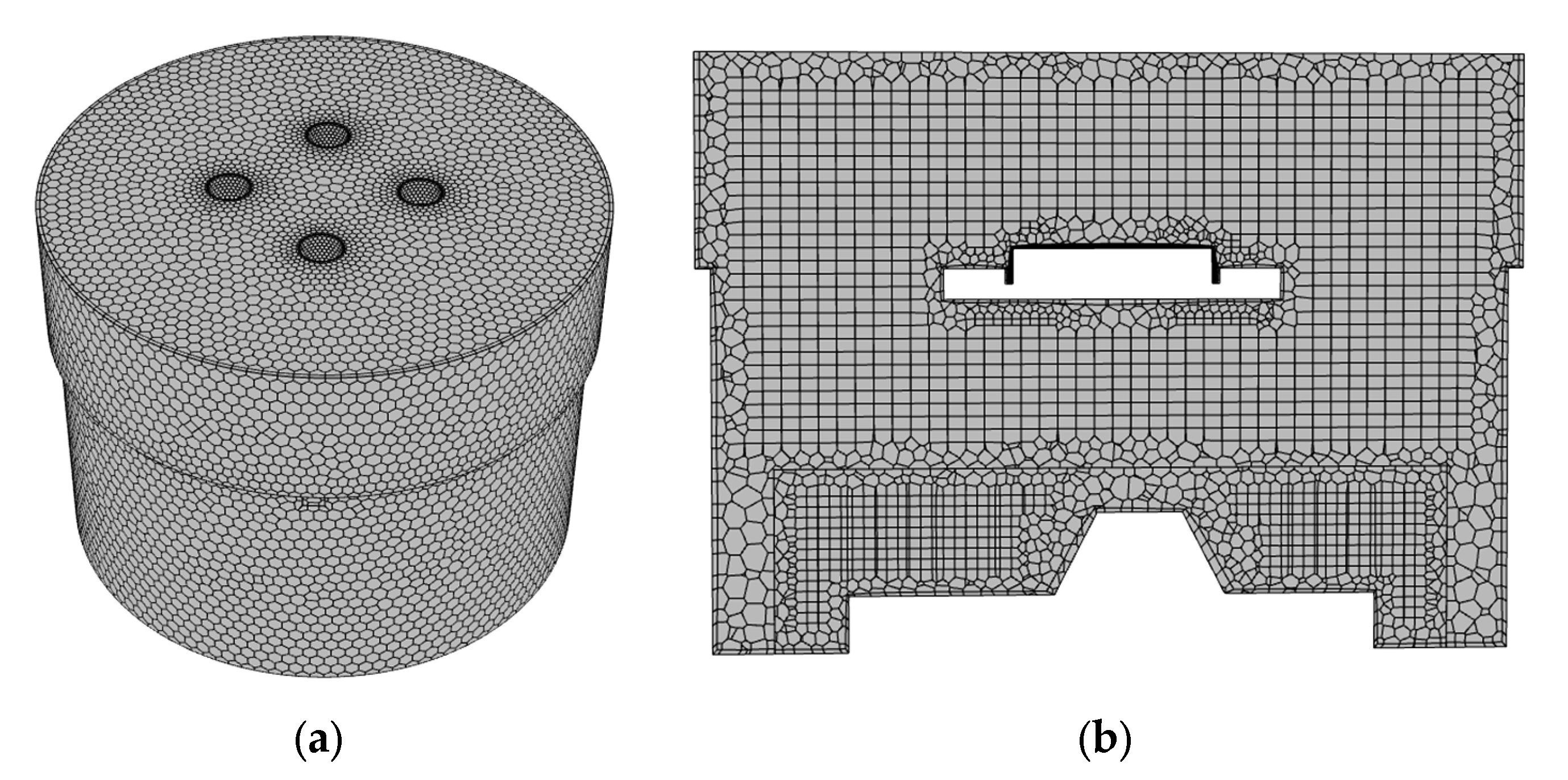
In this section, the CFD model developed to simulate the stirrer and tablet setup is presented. An Ansys Fluent 2022R2 transient, pressure-based solver was used.

3.1. Geometry

Ansys SpaceClaim was used to construct the geometry for the simulation. Figure 2a shows the solid bodies in the beaker: the supported platform (light blue), the stirrer blade (green), and the tablet (pink). Figure 2b shows the fluid domain; the bottom fluid domain (brown) was set to be a moving mesh zone (see Figure 2). This is a significant advance over previous modeling which used a frozen rotor approach [24], as large-scale transient structures, as well as flow interaction with the tablet support structure, can be captured correctly [25]. The lower, cylindrical fluid zone was set as a moving mesh region with a vertical rotation axis, and the mesh motion determined from the rotation rate.

3.2. Computational Mesh

An Ansys fluent watertight geometry meshing tool was used to generate the mesh in the fluid region. The generated mesh has 215,000 cells and comprises poly-hexcore elements with inflation at the walls. Ten layers of fine inflation were used on the tablet to capture the thin concentration boundary layer. Views of the mesh used are given in Figure 3. The minimum orthogonal quality of the mesh is 0.38.
A sensitivity study shows that this mesh gave sufficient resolution. To determine this, two different quantities were examined. Firstly, the overall dependence of the solution on the mesh density was examined by running cases with different mesh densities for stirrer 1 at a tablet Reynolds number of 800 and comparing data after 6 s. These meshes were created by changing both the surface and volume mesh sizes, although the inflation mesh on the tablet was unchanged. Table 1 shows the results, which indicate the power number, a measure of the non-dimensional torque on the stirrer (see later for definition), does not change significantly once the number of cells reaches about 180,000. The Sherwood number, a dimensionless number used in a mass-transfer operation (see later for definition), is unaffected by changes to the mesh in the bulk of the vessel.
Secondly, the inflation mesh on the tablet was changed to reduce the near-wall cell height from 20 μm to 15 μm with the same expansion ratio. This changed the Sherwood number from 376.24 to 376.26, again confirming that the mesh used was adequate.

3.3. Conservation Equations

The mass and momentum conservation equations employed for incompressible flow with a moving mesh are:
· ( u u g ) = 0
( ρ u ) t + · ( ρ ( u u g ) u ) = p + · μ eff ( u + u T )
where μ eff is the sum of the laminar and turbulent dynamic viscosities. The SST k-ω model [26] is chosen as the turbulence model because it performs well even when the turbulence levels are low [27] and the flow is essentially laminar.
The transport equations for the turbulence kinetic energy ( k ) and the turbulence eddy frequency ( ω ) are:
t ( ρ k ) + · ( ρ ( u u g ) k ) = · [ ( μ + μ t σ k 1 ) k ] + P k β * ρ k ω  
  t ( ρ ω ) + · ( ρ   ( u u g ) ω ) = · [ ( μ + μ t σ ω 1 ) ω ] + ( 1 F 1 ) 2 ρ 1 σ ω 2 ω k · ω + α 1 ω k P k β i ρ ω 2  
where σ k 1 = 1.176 , β * = 0.09 ,   σ ω 1 = 2.0 ,   σ ω 2 = 1.168 ,   α 1 = 0.52 and β i = 0.075 .
The turbulence production rate ( P k ) is given by:
  P k = μ t u · ( u + u T )
The blending function, F 1 , is a function of both the near-wall distance and the local values of k and ω;
F 1 = tanh ( Φ 1 4 )  
where
Φ 1 = min ( max ( k β ω y , 500 ν y 2 ω ) , 4 ρ k C D k ω σ ω 2 y 2 )
y is the near-wall distance, ν the kinematic viscosity, and
  C D k ω = max ( 2 ρ 1 σ ω 2 ω k x j ω x j , 1.0 × 10 10 )  
F 1 is expected to be 1.0 inside the boundary layer and zero outside. A second blending function, F 2 , is used to explicitly limit the eddy viscosity inside the boundary layer ( μ t ) [26]
  μ t = α 1 ρ k max ( α 1 ω , S F 2 )
where α 1 is a constant, set to be 0.31. S is the magnitude of the shear strain rate.
The second blending function is given by;
F 2 = tanh ( Φ 2 2 )
where
Φ 2 = max ( 2 k β ω y , 500 ν y 2 ω )
Conservation of species mass gives:
( ρ Y dis ) t + · ( ρ ( u u g ) Y dis ) = · ( ρ D eff Y dye )
where Y dis is the mass fraction for the dissolved species, and D eff is the effective mass diffusion coefficient, given by:
D eff = D + μ t ρ σ Y
where the turbulent Schmidt number is set to the default value of 0.7.

3.4. Model Setup

The mixing vessel was filled with water, with a constant density of 998.2 kg m−3 and a constant viscosity of 0.001 Pa·s. The benzoic acid diffusion coefficient in the water was taken from Irandoust and Andersson [28]. The tablet wall was assumed to have a constant benzoic acid mass fraction of 0.0328 [28]. The rotating speed of the moving fluid domain was set to 100 rpm or 200 rpm corresponding to the stirrer speeds used in the experiment. Each case was run for 20 s with a timestep selected to give 5° of rotation in a single step, which for 200 rpm was 0.66 ms. An additional case was run with no rotation.

3.5. Solution Method

The coupled pressure–velocity scheme was used to solve the equations with the bounded second-order implicit transient formulation. Gradients were determined using the least-squares cell-based option and the pressure was determined using the second-order method. The second-order upwind scheme was used for all the transport equations, except those for turbulence that used the first-order upwind scheme. Converged solutions were achieved when residual values for the continuity, x , y , z velocities and dye were below 10−5. The residual values were calculated based on the locally scaled root mean square (RMS).

4. Results and Discussion

4.1. Flow and Mass Transfer Results from the Simulations

4.1.1. Mass Fraction of Benzoic Acid

The mass fraction contours of benzoic acid at 20 s with different stirrers and rotation speeds are shown in Figure 4. The benzoic acid is more widely distributed at a higher rotation speed with all stirrers. Stirrer 1 provides the most diffused mixing pattern, followed by stirrer 3, while stirrer 2 seems to be the least effective.

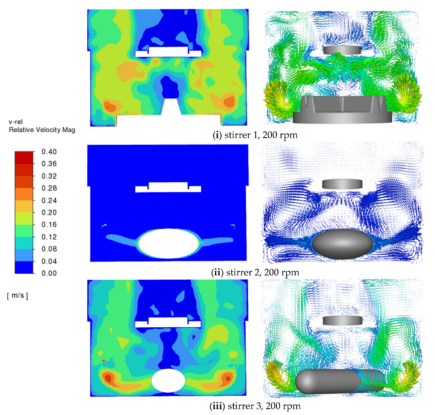
4.1.2. Velocity Field in the Stirrer System

Figure 5 shows the fluid velocity for different stirrers at a stirrer speed of 200 rpm. The velocity magnitude is much higher with stirrers 1 and 3 than with stirrer 2. They range from 0 m/s to 0.4 m/s, which is of the same order of magnitude as in the previous studies conducted by D’Arcy et al. [29], Bai and Armenante [17,18,19], and McCarthy et al. [30]. The complex eddy patterns generated by the stirrers are evident in the vector plot on the right side of the figure. It is also evident that in the region of the tablet the flow is very weak for stirrer 2 and strongest for stirrer 1.

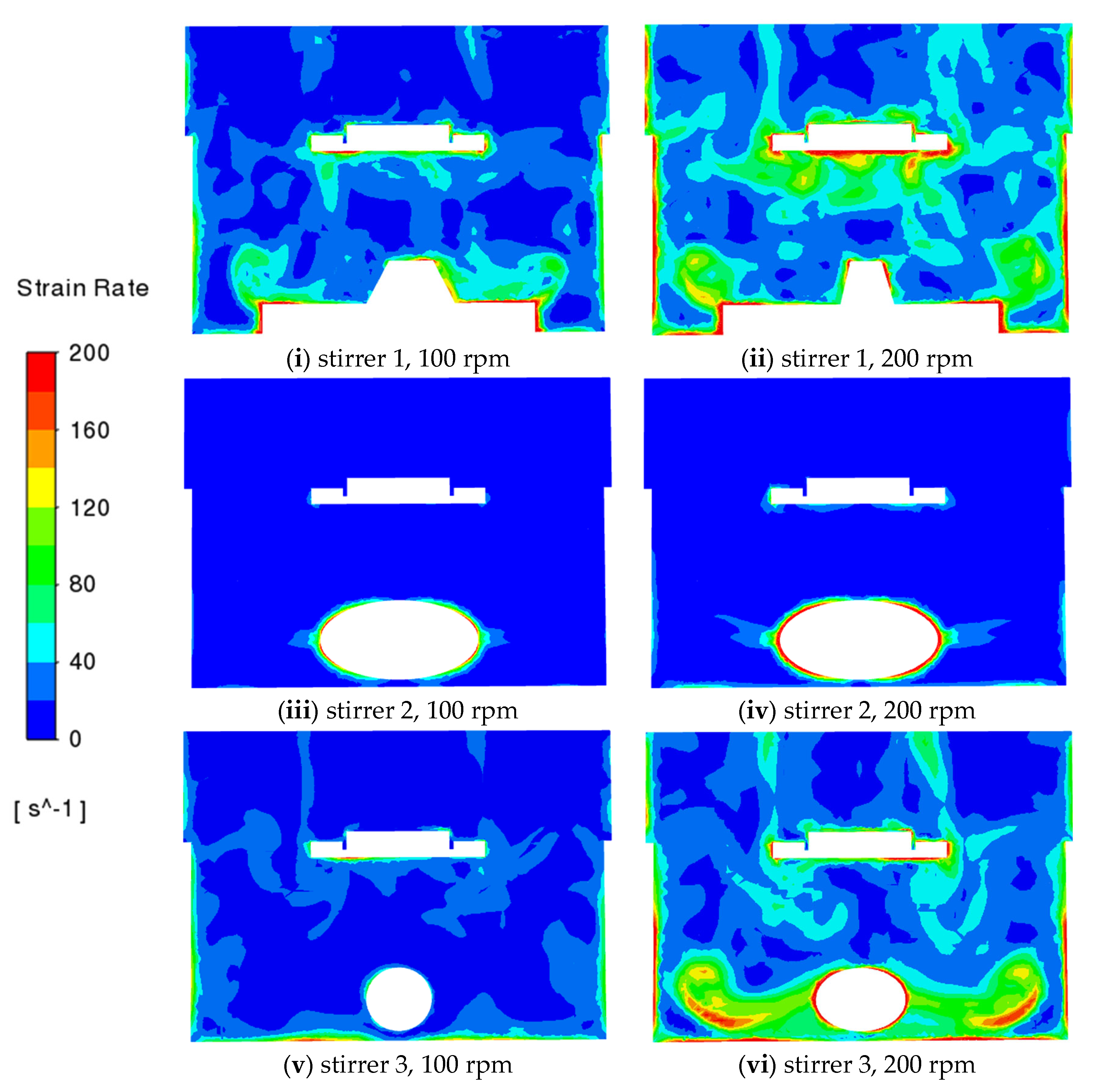
4.1.3. Fluid Strain Rate

The patterns of the fluid strain rate are shown in Figure 6. The strain rate of the fluid ranges from 0 to 200 s−1 while it reaches up to 800 s−1 on the tablet, which is in line with the previous predictions of Bai and Armenante [17,18], and some predicted strain rates for the USP II apparatus shown in Figure 5 of Baxter et al. [20]. The strain rate of the fluid is highest near the tablet with stirrer 1, while it is highest near the stirrer with stirrer 2. The strain rate is important as it controls mixing at the small scale and again illustrates the better performance of stirrer 1.

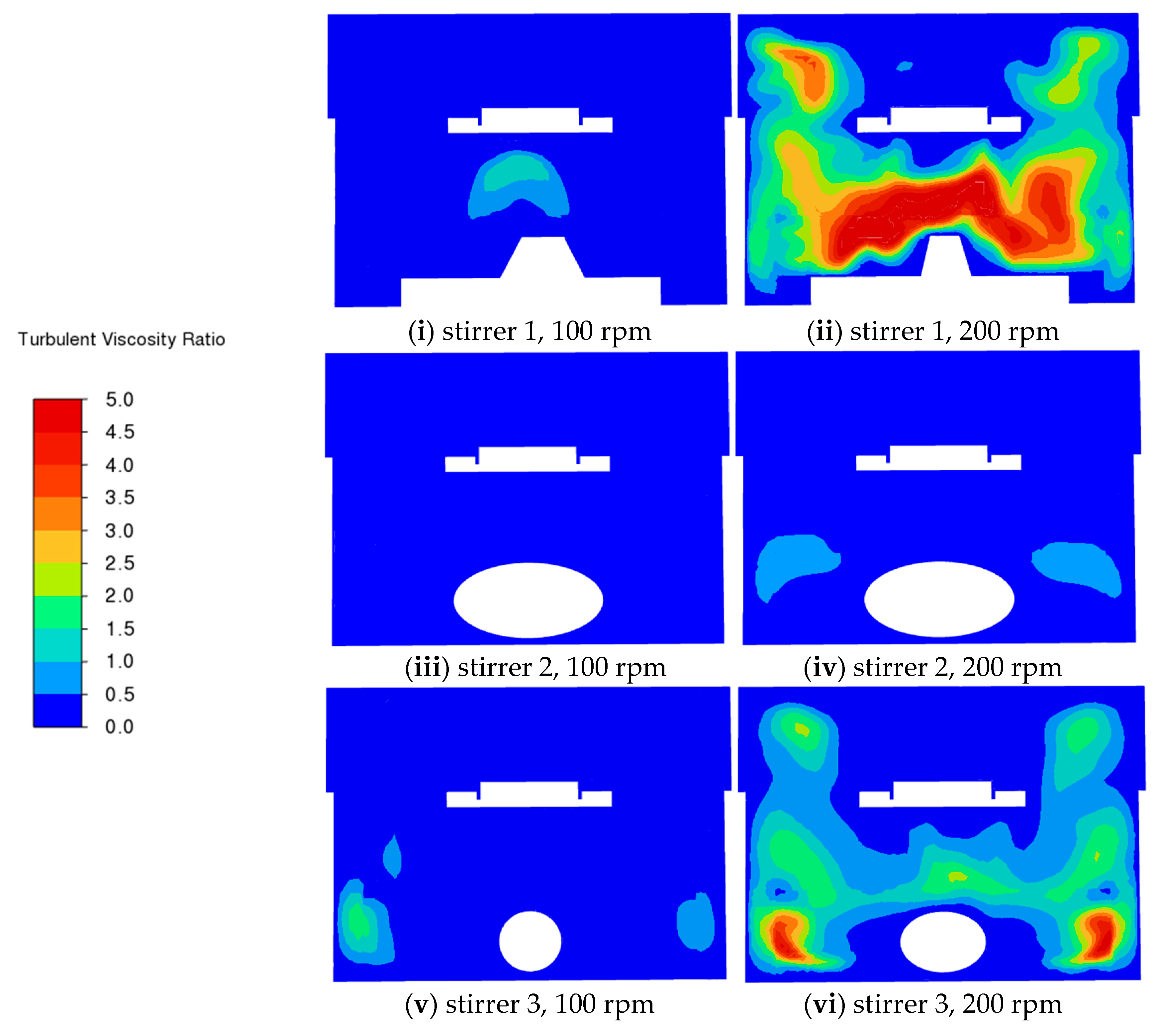
4.1.4. Turbulence Behavior

For all cases studied, the maximum y + value on all walls in the domain is less than 7 overall and far less than unity on the tablet wall. Figure 7 shows the wall y + value on the tablet and stirrer for stirrer 3 rotating at 200 rpm, which is the case with the highest Reynolds number for the tablet, highlighting the very low y +   value on the tablet. Therefore, the first point away from the wall is located in the laminar sublayer and the turbulence equations are integrated to the wall rather than a log-law boundary profile being applied. This is important because it means the mass transfer boundary layer is calculated rather than an incorrect log-law being applied at the very low turbulent Reynolds numbers for the tablet.
Figure 8 shows the contours of the turbulent viscosity ratio, which is the ratio of the turbulent viscosity to the laminar viscosity, in the fluid. The ratio is highest with stirrer 1, followed by stirrer 3, then stirrer 2. With stirrer 1, the highest values are observed above the stirrer. With stirrer 3, the highest values are near the tips of the stirrer. However, in all cases the region around the tablet is largely unaffected by turbulence.
Next, results for the turbulence kinetic energy and turbulence energy dissipation rate are presented. When the rotational speed is 100 rpm, and 200 rpm for stirrer 2, the values are small and close to zero. The turbulence levels are higher, consistent with the observed turbulent eddy viscosity ratio, when the rotational speed is 200 rpm, and are present mainly in the region above the stirrers. Typically, the turbulence kinetic energy ranges from 0 to 0.001 m2 s−2 and the turbulent energy dissipation rate ranges from 0 to 0.1 m2 s−3. These values are consistent with the values obtained in the previous studies conducted by Bai et al. [18,19]. Example plots are provided in Figure 9. It should be noted that the small spikes at the corners where the rotating and stationary frames meet are numerical artefacts that arise for some mesh configurations and are hard to avoid. They arise from the difficulty of matching gradients across interfaces and in this case appear only in the corners of the domain.
It is evident from the results presented above that, while there is some local turbulence in the vicinity of the stirrer and its discharge, the simulations suggest that mass transfer is occurring largely in the laminar regime.

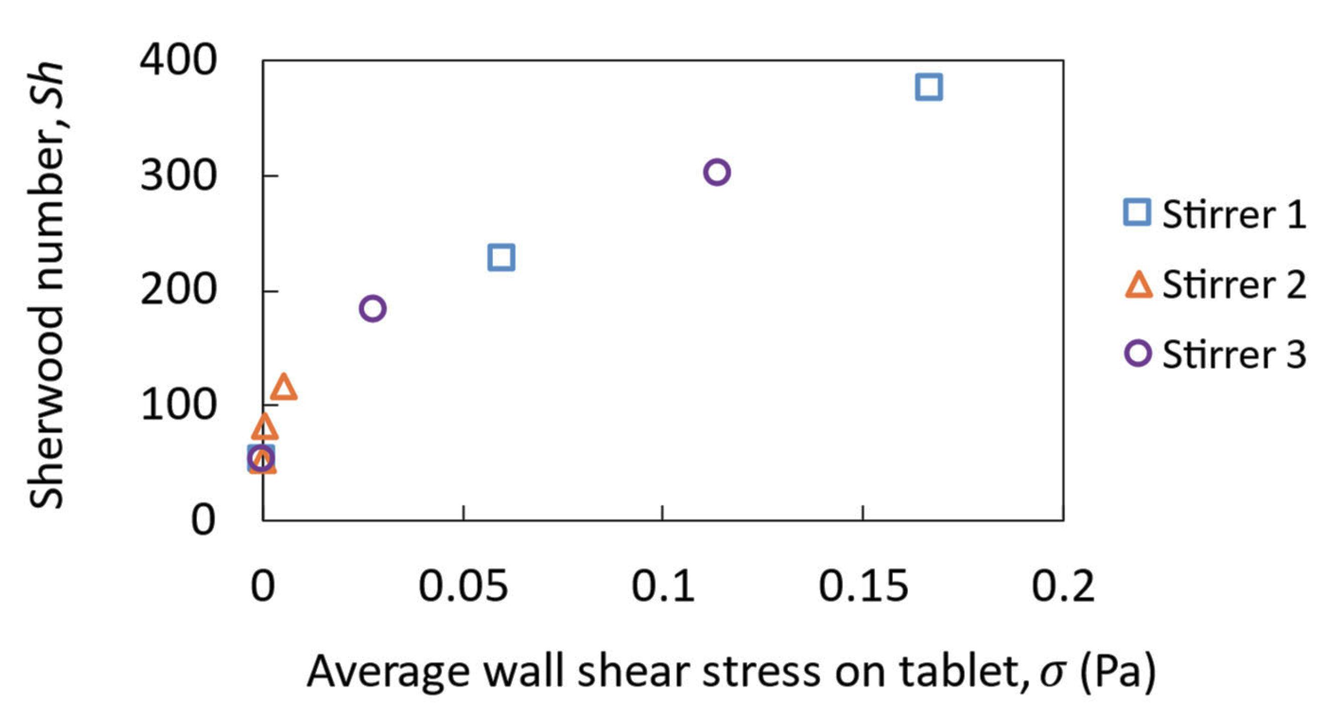
4.2. Comparison with Experimental Data

From basic mass-transfer theory, the mass-transfer rate is related to the mass transfer area; the mass transfer coefficient and the rate of concentration change as defined below:
d   m s o l d   t = A   k   ( C s C b )
where m s o l is the mass of benzoic acid transferred from the tablet to the bulk solution, A is the interfacial area between the tablet and solution, taken as the sum of the top and side areas of the tablet here, k is the overall mass-transfer coefficient, C s is the saturation concentration of benzoic acid at the tablet surface, and C b is the concentration of benzoic acid in the bulk solution, derived from the simulation results. All quantities use kg-m-s units. Data from the last second of the simulation were used to calculate both d   m s o l d   t and C b . The mass-transfer coefficients are calculated from the simulation results using Equation (14) and compared with the experimental results from Langrish et al. [23]. Both experiment and simulation agree that stirrer 1 provides the highest mass-transfer coefficients, followed by stirrer 3 and finally stirrer 2. The values from the simulation are lower than the experimental values overall, but within acceptable ranges. All data are given in Table 2. The mass-transfer coefficients range from 1.33 × 10⁻⁵ to 4.48 × 10⁻⁵ (m s−1) in the experiment and from 6.33 × 10⁻⁶ to 2.89 × 10⁻⁵ (m s−1) in the simulation.
The mass transfer data are further investigated using dimensional analysis, including the calculation of the Reynolds number for the tablet, the Sherwood number, the Schmidt number and the power number.
The Reynolds number for the tablet ( R e t ) is the ratio of inertial forces to viscous forces in the fluid, defined by:
R e t = ρ   u   L t μ = ρ   N   L s   L t 2 μ
where ρ is the density of the solution, μ is the viscosity of the solution, u is the characteristic speed, defined as N   L s / 2   in this study, L t is the length scale of the tablet which is taken as the tablet diameter (0.013 m), L s is the length scale of the impeller which is taken as the impeller diameter (0.034 m for stirrer 1, 0.020 m for stirrer 2 and 0.040 m for stirrer 3), and N is the rotational speed of the stirrer (100 rpm or 200 rpm).
The Sherwood number ( S h ) is the ratio of mass transfer by convection to the mass transfer by diffusion, defined by:
S h = k   L t D
where k is the external mass-transfer coefficient, and D is the diffusivity of the benzoic acid in water.
The Schmidt number ( S c ) is the ratio of momentum diffusivity (kinematic viscosity) over mass diffusivity, defined by:
S c = μ ρ   D
The Ranz–Marshall correlation [31] which is widely used to predict the Sherwood number from a sphere, was used in Langrish et al. [23] to give a reference value. It is used here as a lower bound for estimates of the Sherwood numbers from the experiment and is given by
S h = a + b   R e t c   S c 1 / 3
where a = 2, b = 0.6, and c = 0.5.
The correlations between the Reynolds number for the tablet and the Sherwood number for both the simulations and experiments with different stirrers are shown in Figure 10. The Sherwood numbers for tablet dissolution are of the same order of magnitude as that for spheres when correlated against the Reynolds number for the tablet. The simulation results show good agreement with the experimental data in that they capture the trends for all configurations. Differences can easily be explained by the fact that the magnetic stirrer in the experiment will not rotate perfectly centered on the axis but tend to wobble, causing improved mixing which is consistent with the excellent agreement in the stationary case. Therefore, the statistical significance of the variations between the experimental and simulation data is not included here.
The performance of the stirrers can be examined based on the Reynolds number for the impeller and power number of the impeller [32]. The Reynolds number for the impeller ( R e i ) is given by
R e i = ρ   N   L i 2 μ
The power number ( N p ) is the ratio of the external force exerted over the inertial force imparted, defined by:
N p = P ρ   N 3   L s 5
where P is the external power to the stirrer.
The power ( P ) is determined from the torque ( τ ) derived from the CFD results based on:
P = τ   · 2   π   · N
Figure 11 shows the correlation between the Sherwood number and the impeller Reynolds number. It is found that the Sherwood number increases linearly with the increasing impeller Reynolds number for different stirrers, meaning that the mass-transfer coefficient increases linearly with the increased rotational speed in this system with different stirrers. Stirrer 1 performs best, while stirrers 2 and 3 follow the same trend.
Figure 12 shows the correlation between the Sherwood number and the average wall shear stress on the tablet, which ranges from 0 to 0.2 Pa for different stirrers and different rotational speeds. All data collapse onto a single curve. Typical correlations show that the Sherwood number increases as the wall shear stress increases and this is evident here too.
Figure 13 shows the relationship between the power number and impeller Reynolds number for different stirrers and different rotational speeds. With stirrer 2, the Reynolds numbers are smaller than 2000, and the power number decreases with an increase in the Reynolds number showing laminar flow behavior. With stirrer 1, the Reynolds numbers are in the range of 2000 to 4000 and the power number decreases slowly as the Reynolds number increases. With stirrer 3, the Reynolds numbers range from 3000 to 6000 and the power number only changes slightly when the Reynolds number increases. These results are consistent with those expected from compilations of data for many impellers [32].

4.3. Overall Discussion

The link between pharmaceutical dissolution (upon which this modeling is based) and food is that the mass-transfer coefficients for pharmaceutical components and food components are only slightly dependent on the nature of the solute, and the mass-transfer coefficients for different solutes may be related to each other through the use of the Sherwood number, as shown in Cussler [33], and Langrish et al. [23]. Therefore, mass-transfer coefficients measured and simulated for pharmaceutical components are directly relevant to mass-transfer coefficients for food components.
The gap between this work and that of previous work (D’Arcy et al. [21,22,29]) reflects both the realization of the similarities between mass transfer for food components and for pharmaceutical ones [34], and the improvements in computational simulation techniques that have occurred in the intervening period [24,26,27], including the simulation here of the wall shear stresses above the tablet surfaces.
While beyond the scope of this work, tablet hardness may affect the breakup of tablets and therefore the length scales and mass-transfer coefficients from tablets. Only a single tablet hardness was used throughout all the experimentation used in this work.

5. Conclusions

This study presents CFD simulations of an in vitro beaker and stirrer system. This system was investigated extensively about 15 years ago using much simpler CFD approaches and did not include mass transfer simulations. Here, a CFD model is developed that accounts for the rotation of the stirrer in as complete a way as possible and additionally models simultaneous mass transfer. The sliding mesh approach captures transient interactions of the flow with the support structure and the tablet.
The estimated mass-transfer coefficients from the simulation match well with the experimental results. Tablet dissolution and mixing behaviors of the system are influenced by both the type of stirrer and the rotation speed. The dimensionless mass-transfer coefficient (the Sherwood number, which ranges from 53 to 376) correlates well with the tablet Reynolds numbers (0 to 938) and the shear stress (0 to 0.167 Pa) acting on the tablet. The correlations between the power number (0.0061 to 0.196) and the impeller Reynolds number (719 to 5715) are also presented for different stirrers and follow the expected trends. This work reinforces the utility of CFD simulation to provide additional insights into the dissolution process and has the capability of modeling the digestion process, at the food particle scale.

Author Contributions

Conceptualization, T.A.G.L.; methodology (experiments), T.A.G.L., C.Z.; software (CFD), X.L., D.F.F.; formal analysis, T.A.G.L., X.L., D.F.F., C.Z.; writing—original draft preparation, X.L.; writing—review and editing, T.A.G.L., D.F.F. All authors have read and agreed to the published version of the manuscript.

Funding

This work was partially supported by the Australian Research Council Training center for Australian food processing industry in the 21st century (IC140100026).

Informed Consent Statement

Not applicable so would like to exclude this statement.

Data Availability Statement

The data that support the findings of this study are available from the corresponding author upon reasonable request.

Acknowledgments

The authors acknowledge the use of the National Computational Infrastructure (NCI) which is supported by the Australian Government, and accessed through the Sydney Informatics Hub HPC Allocation Scheme, which is supported by the Deputy Vice-Chancellor (Research), University of Sydney. X.L. and C.Z. received an Australian Government Research Training Program Stipend Scholarship and a supplementary scholarship from the Centre for Advanced Food Engineering (CAFE) of the University of Sydney.

Conflicts of Interest

The authors declare no conflict of interest. One of the authors (DFF) consults users of the Ansys software, but this has not influenced the views expressed here.

References

  1. Koch, W.F.; Ma, B. The US Pharmacopeia: Interfacing Chemical Metrology with Pharmaceutical and Compendial Science. Accredit. Qual. Assur. 2011, 16, 43–51. [Google Scholar] [CrossRef]
  2. Li, C.; Yu, W.; Wu, P.; Chen, X.D. Current in Vitro Digestion Systems for Understanding Food Digestion in Human Upper Gastrointestinal Tract. Trends Food Sci. Technol. 2020, 96, 114–126. [Google Scholar] [CrossRef]
  3. Zhong, C.; Langrish, T. A Comparison of Different Physical Stomach Models and an Analysis of Shear Stresses and Strains in These System. Food Res. Int. 2020, 135, 109296. [Google Scholar] [CrossRef]
  4. D’Arcy, D.M.; Liu, B.; Bradley, G.; Healy, A.M.; Corrigan, O.I. Hydrodynamic and Species Transfer Simulations in the USP 4 Dissolution Apparatus: Considerations for Dissolution in a Low Velocity Pulsing Flow. Pharm. Res. 2010, 27, 246–258. [Google Scholar] [CrossRef]
  5. Vardakou, M.; Mercuri, A.; Barker, S.A.; Craig, D.Q.M.; Faulks, R.M.; Wickham, M.S.J. Achieving Antral Grinding Forces in Biorelevant In Vitro Models: Comparing the USP Dissolution Apparatus II and the Dynamic Gastric Model with Human In Vivo Data. AAPS PharmSciTech 2011, 12, 620–626. [Google Scholar] [CrossRef] [PubMed]
  6. Kong, F.; Singh, R.P. A Model Stomach System to Investigate Disintegration Kinetics of Solid Foods during Gastric Digestion. J. Food Sci. 2008, 73, 202–210. [Google Scholar] [CrossRef] [PubMed]
  7. Molly, K.; Woestyne, M.V.; De Smet, I.; Verstraete, W. Validation of the Simulator of the Human Intestinal Microbial Ecosystem (SHIME) Reactor Using Microorganism-Associated Activities. Microb. Ecol. Health Dis. 1994, 7, 191–200. [Google Scholar] [CrossRef]
  8. Yoo, M.J.Y.; Chen, X.D. GIT Physicochemical Modeling—A Critical Review. Int. J. Food Eng. 2007, 2, 4. [Google Scholar] [CrossRef]
  9. Verhoeckx, K.; Cotter, P.; López-Expósito, I.; Kleiveland, C.; Lea, T.; Mackie, A.; Requena, T.; Swiatecka, D.; Wichers, H. The Impact of Food Bioactives on Health; Springer International Publishing: Cham, Switzerland, 2015; ISBN 978-3-319-15791-7. [Google Scholar]
  10. Polo, A.; Cappello, C.; Carafa, I.; Da Ros, A.; Baccilieri, F.; Di Cagno, R.; Gobbetti, M. A Novel Functional Herbal Tea Containing Probiotic Bacillus Coagulans GanedenBC30: An in Vitro Study Using the Simulator of the Human Intestinal Microbial Ecosystem (SHIME). J. Funct. Foods 2022, 88, 104873. [Google Scholar] [CrossRef]
  11. Chen, J.; Gaikwad, V.; Holmes, M.; Murray, B.; Povey, M.; Wang, Y.; Zhang, Y. Development of a Simple Model Device for in Vitro Gastric Digestion Investigation. Food Funct. 2011, 2, 174–182. [Google Scholar] [CrossRef]
  12. Tran Do, D.H.; Kong, F.; Penet, C.; Winetzky, D.; Gregory, K. Using a Dynamic Stomach Model to Study Efficacy of Supplemental Enzymes during Simulated Digestion. LWT 2016, 65, 580–588. [Google Scholar] [CrossRef]
  13. Guerra, A.; Denis, S.; le Goff, O.; Sicardi, V.; François, O.; Yao, A.F.; Garrait, G.; Manzi, A.P.; Beyssac, E.; Alric, M.; et al. Development and Validation of a New Dynamic Computer-Controlled Model of the Human Stomach and Small Intestine. Biotechnol. Bioeng. 2016, 113, 1325–1335. [Google Scholar] [CrossRef]
  14. Passannanti, F.; Nigro, F.; Gallo, M.; Tornatore, F.; Frasso, A.; Saccone, G.; Budelli, A.; Barone, M.V.; Nigro, R. In Vitro Dynamic Model Simulating the Digestive Tract of 6-Month-Old Infants. PLoS ONE 2017, 12, e0189807. [Google Scholar] [CrossRef]
  15. Armenante, P.; Muzzio, F. Inherent Method Variability in Dissolution Testing: The Effect of Hydrodynamics in the USP II Apparatus. A Technical Report Submitted to the Food and Drug Administration. 2005. Available online: https://www.google.com/url?sa=t&rct=j&q=&esrc=s&source=web&cd=&cad=rja&uact=8&ved=2ahUKEwjuxbXmv4L9AhVKhlYBHZnFAEgQFnoECA0QAQ&url=https%3A%2F%2Fwww.semanticscholar.org%2Fpaper%2FInherent-Method-Variability-in-Dissolution-Testing-Armenante%2F8f74093fc97456c07faf4c79b9a13a0281cdd4ad&usg=AOvVaw1dwSSOsLXtoaWZ9_7MO0Up (accessed on 1 January 2023).
  16. Bai, G.; Wang, Y.; Armenante, P.M. Velocity Profiles and Shear Strain Rate Variability in the USP Dissolution Testing Apparatus 2 at Different Impeller Agitation Speeds. Int. J. Pharm. 2011, 403, 1–14. [Google Scholar] [CrossRef]
  17. Bai, G.E.; Armenante, P.M. Hydrodynamic, Mass Transfer, and Dissolution Effects Induced by Tablet Location during Dissolution Testing. J. Pharm. Sci. 2009, 98, 1511–1531. [Google Scholar] [CrossRef]
  18. Bai, G.; Armenante, P.M. Velocity Distribution and Shear Rate Variability Resulting from Changes in the Impeller Location in the USP Dissolution Testing Apparatus II. Pharm. Res. 2008, 25, 320–336. [Google Scholar] [CrossRef]
  19. Bai, G.; Armenante, P.M.; Plank, R.V.; Gentzler, M.; Ford, K.; Harmon, P. Hydrodynamic Investigation of USP Dissolution Test Apparatus II. J. Pharm. Sci. 2007, 96, 2327–2349. [Google Scholar] [CrossRef]
  20. Baxter, J.L.; Kukura, J.; Muzzio, F.J. Hydrodynamics-Induced Variability in the USP Apparatus II Dissolution Test. Int. J. Pharm. 2005, 292, 17–28. [Google Scholar] [CrossRef]
  21. D’Arcy, D.M.; Corrigan, O.I.; Healy, A.M. Hydrodynamic Simulation (Computational Fluid Dynamics) of Asymmetrically Positioned Tablets in the Paddle Dissolution Apparatus: Impact on Dissolution Rate and Variability. J. Pharm. Pharmacol. 2005, 57, 1243–1250. [Google Scholar] [CrossRef]
  22. D’Arcy, D.M.; Corrigan, O.I.; Healy, A.M. Evaluation of Hydrodynamics in the Basket Dissolution Apparatus Using Computational Fluid Dynamics—Dissolution Rate Implications. Eur. J. Pharm. Sci. 2006, 27, 259–267. [Google Scholar] [CrossRef]
  23. Langrish, T.A.G.; Zhong, C.; Sun, L. Probing Differences in Mass-Transfer Coefficients in Beaker and Stirrer Digestion Systems and the USP Dissolution Apparatus 2 Using Benzoic Acid Tablets. Processes 2021, 9, 2168. [Google Scholar] [CrossRef]
  24. Aubin, J.; Fletcher, D.F.; Xuereb, C. Modeling Turbulent Flow in Stirred Tanks with CFD: The Influence of the Modeling Approach, Turbulence Model and Numerical Scheme. Exp. Therm. Fluid Sci. 2004, 28, 431–445. [Google Scholar] [CrossRef]
  25. Luo, J.Y.; Gosman, A.D.; Issa, R.I.; Middleton, J.C.; Fitzgerald, M.K. Full Flow Field Computation of Mixing in Baffled Stirred Vessels. Chem. Eng. Res. Des. 1993, 71, 342–344. [Google Scholar]
  26. Menter, F.R. Two-Equation Eddy-Viscosity Turbulence Models for Engineering Applications. AIAA J. 1994, 32, 1598–1605. [Google Scholar] [CrossRef]
  27. Menter, F.R. Review of the Shear-Stress Transport Turbulence Model Experience from an Industrial Perspective. Int. J. Comut. Fluid Dyn. 2009, 23, 305–316. [Google Scholar] [CrossRef]
  28. Irandoust, S.; Andersson, B. Concentration-dependent Diffusivity of Benzoic Acid in Water and Its Influence on the Liquid–Solid Mass Transfer. Can. J. Chem. Eng. 1986, 64, 954–959. [Google Scholar] [CrossRef]
  29. D’Arcy, D.M.; Healy, A.M.; Corrigan, O.I. Towards Determining Appropriate Hydrodynamic Conditions for in Vitro in Vivo Correlations Using Computational Fluid Dynamics. Eur. J. Pharm. Sci. 2009, 37, 291–299. [Google Scholar] [CrossRef]
  30. McCarthy, L.G.; Bradley, G.; Sexton, J.C.; Corrigan, O.I.; Healy, A.M. Computational Fluid Dynamics Modeling of the Paddle Dissolution Apparatus: Agitation Rate, Mixing Patterns, and Fluid Velocities. AAPS PharmSciTech 2004, 5, 50–59. [Google Scholar] [CrossRef]
  31. Ranz, W.E.; Marshall, W.R., Jr. Evaporation from Drops—Part II. Chem. Eng. Prog. 1952, 48, 173–180. [Google Scholar]
  32. Hemrajani, R.R.; Tatterson, G.B. Mechanically Stirred Vessels. In Handbook of Industrial Mixing; John Wiley & Sons, Inc.: Hoboken, NJ, USA, 2004; pp. 345–390. ISBN 0471451452. [Google Scholar]
  33. Cussler, E.L. Diffusion: Mass Transfer in Fluid Systems, 2nd ed.; Cambridge University Press: Cambridge, UK, 1997; ISBN 9780521871211. [Google Scholar]
  34. Langrish, T.A.G. Multifilm Mass Transfer and Time Constants for Mass Transfer in Food Digestion: Application to Gut-on-chop Models. Appl. Biosci. 2022, 1, 101–112. [Google Scholar] [CrossRef]
Figure 1. Dimensions of the three stirrers that were used in the experiments. (a) stirrer 1; (b) stirrer 2; (c) stirrer 3.
Processes 11 00505 g001
Figure 2. Geometry of the beaker and stirrer system and the fluid domain with stirrer 1 (a) solid bodies; (b) fluid domain.
Processes 11 00505 g002
Figure 3. Computational mesh on the fluid domain with stirrer 1. (a) surface mesh. (b) section through the vessel.
Processes 11 00505 g003
Figure 4. CFD predictions of the benzoic acid mass fraction on the vertical middle cross-section for different stirrers at different rotation speeds (100 rpm and 200 rpm).
Processes 11 00505 g004
Figure 5. CFD predictions of velocity magnitude contour on the vertical middle cross-section for different stirrers at different rotation speeds (100 rpm and 200 rpm).
Processes 11 00505 g005
Figure 6. CFD predictions of strain rate on the vertical middle cross-section for different stirrers at different rotation speeds (100 rpm and 200 rpm).
Processes 11 00505 g006
Figure 7. CFD predictions of the wall y+ value on (a) the surface of the tablet; and (b) the surface of the stirrer and the base of the beaker for the stirrer 3 system with a rotation speed of 200 rpm.
Processes 11 00505 g007
Figure 8. CFD predictions of the turbulent viscosity ratio on the vertical middle cross-section for different stirrers at different rotation speeds (100 rpm and 200 rpm).
Processes 11 00505 g008
Figure 9. Turbulence kinetic energy (left) and turbulence energy dissipation rate (right) for stirrers 1 and 3 operating at 200 rpm.
Processes 11 00505 g009
Figure 10. The relationship between the Sherwood number and Reynolds number for the tablet achieved from experimental and simulation results. The experimental data are taken from Langrish et al. [23].
Processes 11 00505 g010
Figure 11. Sherwood number as a function of the impeller Reynolds number derived from the simulation results.
Processes 11 00505 g011
Figure 12. Sherwood number as a function of the average wall shear stress derived from the simulation results.
Processes 11 00505 g012
Figure 13. Power number as a function of the impeller Reynolds number derived from the simulation results.
Processes 11 00505 g013
Table 1. Results of the mesh independence study.
Number of CellsPower NumberSherwood Number
107,0000.193376.30
179,0000.184376.20
215,0000.181376.24
233,0000.184376.19
243,0000.180376.26
Table 2. Comparison of estimated mass transfer coefficients (m s−1) between experimental and simulation results. The experimental data are taken from Langrish et al. [23].
Speed (rpm)Stirrer 1Stirrer 2Stirrer 3
ExperimentSimulationExperimentSimulationExperimentSimulation
05.21 × 10⁻⁶,
4.55 × 10⁻⁶
4.11 × 10⁻⁶
1003.86 × 10−5, 3.60 × 10−51.74 × 10−51.56 × 10⁻⁵,
1.33 × 10⁻⁵
6.33 × 10−62.23 × 10−5,
1.94 × 10⁻⁵
1.40 × 10⁻⁵
2004.48 × 10−5,
4.33 × 10⁻⁵
2.89 × 10−51.87 × 10−5, 1.48 × 10−58.99 × 10−63.47 × 10⁻⁵, 3.44 × 10−52.32 × 10−5
Disclaimer/Publisher’s Note: The statements, opinions and data contained in all publications are solely those of the individual author(s) and contributor(s) and not of MDPI and/or the editor(s). MDPI and/or the editor(s) disclaim responsibility for any injury to people or property resulting from any ideas, methods, instructions or products referred to in the content.

