Industrial Application of Data-Driven Process Monitoring with an Automatic Selection Strategy for Modeling Data

Abstract

The increasing scale of industrial processes has significantly motivated the development of data-driven fault detection and diagnosis techniques. The selection of representative fault-free modeling data from operation history is an important prerequisite to establishing a long-term effective process monitoring model. However, industrial data are characterized by a high dimension and multimode, and are also contaminated with both outliers and frequent random disturbances, making automatic modeling data selection a great challenge in industrial applications. In this work, an information entropy-based automatic selection strategy for modeling data is proposed, based on which a general real-time process monitoring framework is developed for a large-scale industrial methanol to olefin unit with multiple operating conditions. Modeling data representing normal operating conditions are automatically selected with only a few manually defined normal samples. A long-term effective process monitoring model is then established based on a multi-layer autoencoder, through which unexpected disturbances in real-time operation can be detected early and the root cause can be preliminarily diagnosed by contribution plots. The adjustment of operating conditions has also been considered through a model update strategy. Details of the proposed data selection strategy and modeling process have been provided to facilitate the industrial application of process monitoring systems by other researchers or companies.

1. Introduction

Demands on process safety continue to rise due to the ever-increasing scale and complexity of the modern process industry. Aiming at this issue, the process monitoring technique was designed as a powerful tool to ensure the long-term stable operation of industrial systems through Fault detection and diagnosis (FDD). FDD aims to early detect the abnormal behaviors of the process and transfer the fault information to operators to minimize the impact of faults [1]. Over the past decades, process monitoring has been well developed and divided into model-based methods, knowledge-based methods, and data-driven methods [2,3,4]. As the real-time operation of plant-wide processes becomes much more complex than that under ideal conditions, many random factors cannot be considered in model-based methods and knowledge-based methods, which challenges their application in industrial FDD systems. Given the widespread application of sensors and data transmission techniques, data-driven process monitoring methods have attracted increasing attention in the past two decades from both academia and industry [1,4,5,6,7].

Multivariate statistical analysis is one of the most commonly used techniques in data-driven process monitoring, which is known as multivariate statistical process monitoring (MSPM). MSPM methods aim to project original data into a low-dimensional feature space and a residue space. Then, statistics are employed as the dissimilarity measure in each subspace to determine a control limit for normal variations. The most classical methods include principal component analysis (PCA), partial least squares [8], canonical variate analysis [9], and independent component analysis [10], which are applicable to monitor multivariate linear processes. To handle nonlinear processes, numerous variants of these MSPM methods, such as kernel PCA [11], have been developed by mapping original data into a higher-dimensional linearly separable space. More kernel-based MSPM methods proposed to handle nonlinear characteristics can be referred to in Apsemidis’s review [12]. In addition, industrial processes also have obvious process dynamics, which are ignored by traditional methods. Ku proposed dynamic PCA to extract the autocorrelation of variables with an augmented matrix [13], but the selection of time lag is an ad hoc solution. As an alternative, the dynamic latent variable method is further proposed to handle process dynamics, in which auto-regressive PCA and a vector autoregressive model are combined to extract autocorrelation as well as static cross-correlation [14]. Dong and Qin extend it with a dynamic inner PCA to capture the most dynamic variations in the data [15]. More applications of dynamic latent variable models in process monitoring can be referred to in Zheng’s review paper [16]. Although MSPM methods and their variants have made great progress, multivariate statistical models may not be sufficient to extract complex data characteristics for processes with high nonlinearity and process dynamics.

More recently, deep learning methods, as one of the most popular research interests, have been gradually applied to process monitoring domains. Deep learning methods employ multi-layer artificial neural networks (ANN) to extract features from data. The introduction of nonlinear activation functions enables ANN to approximate complex nonlinear relationships. In this scope, the autoencoder, a special ANN whose output value is equal to its input value, has been proven to be a more effective dimensionality reduction and reconstruction method than PCA [17]. Later, the autoencoder was applied to anomaly detection [18] and unsupervised fault detection [19]. To improve the performance of process monitoring, numerous extensions to the autoencoder have been developed. A stacked autoencoder was widely applied to process monitoring because of the good performance of the deep neural network in feature extraction [20,21]. Yu and Zhao applied a denoising autoencoder for robust process monitoring [22]. The variational autoencoder was proposed by Kingma and Welling as a regularized autoencoder in which the distribution of latent variables is restricted to a normal distribution to prevent overfitting [23]. Based on the variational autoencoder, Cheng et al. constructed a recursive neural network instead of ANN to extract process dynamics [24]. Zhang and Qiu proposed a dynamic-inner autoencoder, in which a vector autoregressive model is integrated into a convolutional autoencoder to capture process dynamics [25].

The aforementioned methods have been widely applied for process monitoring proposes, while most of them require a fully labeled training dataset [26], which is a huge challenge for their real application in monitoring large-scale industrial processes [27]. A plant-wide process generally contains several operation units and complex automatic control systems, resulting in numerous process variables and complex correlations among them [28,29]. Moreover, there are multiple operating conditions according to the adjustment of production loads [30,31], and certain variables also show nonstationary characteristics due to various factors, such as equipment aging [32]. Given these complex data characteristics, it is difficult to define the normal operating conditions and label fault-free samples from massive historical data to establish a long-term effective process monitoring model. Different from simulation processes such as the Tennessee Eastman process that the training data have already been provided, there are many outliers in historical data of industrial processes that have to be labeled and excluded before training the process monitoring model. To label data manually is expensive due to the high labor and time costs [33]. Therefore, automatic data labeling with limited labeled samples from normal operating conditions has become an important research direction. This issue can be regarded as a positive-unlabeled learning problem [34]. The positive-unlabeled learning has already been applied to handle fault detection and classification tasks with only a few normal samples labeled [26,35,36,37]. The most important task in positive-unlabeled learning is to determine the distribution range of normal samples to label outliers in historical data [38]. Euclidean distance is a commonly used similarity measure for multivariate sequences based on the distance between normal samples and fault samples [39,40]. Hu et al. applied KL-divergence to label fault samples from a large amount of historical data according to the distribution information of multivariate data [41]. However, the potential information contained in the data space structure of the unlabeled samples has not been considered in data labeling by the above methods [38]. Then, semi-supervised deep learning was further introduced to deal with the process monitoring issue [42,43]. Qian et al. proposed a positive-unlabeled learning based on a hybrid network, which contains a classifier, a feature extraction module, and a clustering layer. An optimization strategy is designed for these three modules to achieve promising fault detection performance using only a few labeled normal samples [26]. Zheng and Zhao proposed a three-step high-fidelity positive-unlabeled approach based on deep learning [35], in which a self-training stacked autoencoder is utilized for data labeling. Although these methods have been applied to handle the fault detection task with limited data labels, most of them were applied to benchmark simulation processes, and there are still several issues that limit their application in plant-wide industrial processes [44]. Unlike simulation processes where most variables display a relatively stable variation, the range of variable variations in industrial processes is much wider. There are frequent random disturbances during practical operation, and only a few key variables, which have a significant impact on product quality, are controlled within a small interval. Therefore, when applying multivariate sequence similarity measures for data labeling, there could be situations where the distance between normal samples is larger than that between normal samples and faults, which will lead to a large control limit for normal variations. The fault samples could be labeled as normal samples together with the normal disturbances in historical data. The real faults will be buried in these normal disturbances and hard to be detected by the process monitoring method in the online application. Moreover, there are a large number of trainable parameters in semi-supervised deep learning models. For a process with very few labeled normal samples, the number of initial training samples is not enough to build an effective deep learning model. Further, the labeled samples obtained by the semi-supervised model are not reliable, which leads to a poor generalization ability of the final process monitoring model.

To address these issues, an automatic selection strategy for modeling data is proposed and applied in the development of an industrial process monitoring framework. The main contributions of this work include: (1) An information entropy-based automatic data selection strategy is proposed to label normal samples and fault samples in historical data. It only requires a very small part of normal samples to be labeled, and all other samples in the historical data, whether normal samples or fault samples are unlabeled. The proposed strategy labels samples through the dissimilarity measure between the distribution of key variables in labeled normal samples and that in unlabeled samples using information entropy within a sliding window. In this way, only abnormal behaviors that affect the key variables will be labeled as fault samples, while the random disturbances that occur in other variables will be labeled as normal samples as long as the pre-defined process operation has not been impacted. Moreover, an accurate estimation of the distribution of variables in each sliding window can be obtained by information entropy with proper window width. Therefore, the proposed strategy does not require a significant number of training samples as deep learning methods to achieve effective data labeling performance. (2) Based on the labeled samples from the proposed data selection strategy, a multi-layer autoencoder and the contribution plots are established for fault detection and diagnosis, in which a model update strategy is proposed to handle the multimode issue. Generally, the multimode issue is addressed under the assumption that all possible modes of the process are available in historical data, while it is hard to be satisfied in industrial processes. Considering that the switching of the mode mostly results from the adjustment of production loads, which can be easily identified by the contribution plots, a mode update strategy is utilized in the proposed methods to monitor multimode processes by adjusting the model parameters according to the fault diagnosis results. The proposed method can be applied to monitor multimode processes with only one mode given in historical data. (3) The proposed method is verified through an industrial application on a methanol-to-olefin facility, which contains both reaction and regeneration units with more than 150 process variables. Given only 1440 labeled normal samples, the proposed automatic data selection strategy achieves correct data labeling for a large unlabeled historical dataset. Then, the process monitoring model is established and successfully tested through about three months (120,000 samples) of real-time application. Details on common procedures of industrial process monitoring systems, including data preprocessing, offline modeling, and real-time monitoring, have also been provided to demonstrate the generalization and replicability of the proposed method.

The following parts of this paper are organized as follows: the preliminaries of the proposed method are introduced in Section 2. The proposed automatic selection strategy for modeling data and the procedures of the proposed industrial process monitoring framework are introduced in Section 3. An industrial application of the proposed method on a methanol to olefin unit of a real chemical plant is presented in Section 4. The conclusions are drawn in Section 5.

2. Preliminaries

In this section, algorithms and theoretical basis applied in this work are introduced as preliminaries.

2.1. Information Entropy

Information entropy is applied in this work as a dissimilarity measure to label normal samples and fault samples in the historical dataset. Given a time series of variable $x\left(x_1,x_2,\dots ,x_l,\dots ,x_n\right)$, information entropy can be calculated as follows [45],

$$H\left(x\right)=-{\displaystyle \sum }_{i=1}^{n}p\left(x_i\right)\log \left(p\left(x_i\right)\right)$$

(1)

where $p\left(x_i\right)$ is probability density function. $p\left(x_i\right)$ can be estimated by a few methods, and kernel density estimation is employed in this work. As shown in Equation (2), a probability density function can be estimated by a kernel function $K\left(·\right)$ for each available sample in the variable $x$, and the final probability density function $p\left(x\right)$ is obtained by averaging all these probability density functions,

$$P\left(x\right)=\frac{1}{n}{\displaystyle \sum }_{i=1}^{n}K\left(x-x_i\right)=\frac{1}{\sqrt{2\pi }nd}{\displaystyle \sum }_{i=1}^{n}K(-\frac{{\left(x-x_i\right)}^2}{2d^2})$$

(2)

where $K\left(\cdot \right)$ is the kernel function, and $d$ is the window width, which is usually determined using Silverman’s rule [46].

2.2. Autoencoder

An autoencoder is a special ANN structure, which contains an encoder and a decoder. As shown in Figure 1, the encoder is used to map the input data into hidden layers with activation functions, by which the feature of the input data can be extracted. Then, the decoder is used to reconstruct the input data with the hidden features extracted by the encoder. The autoencoder aims to minimize the error between the output values and the input values.

When an autoencoder has been trained with normal data, the reconstruction error of new test data will be kept within a certain range, and the sample whose reconstruction error exceeds that range will be considered a fault sample, by which the fault detection is implemented. Because of the fitting ability of ANN, the autoencoder has a good performance in handling process nonlinearity. There could be multiple ANN layers in the encoder and the decoder, and the fitting ability could be improved with the increase in the number of layers and neurons. It is worth noting that good performance can only be achieved when sufficient training samples are given; otherwise, it will lead to overfitting, and the model cannot be generalized to new test data.

2.3. Industrial Process Monitoring Procedure

In simulation processes, the development of feature extraction algorithms is usually the research focus that determines the process monitoring performance. In contrast, the data preprocessing and the selection of modeling data are rarely considered because the training dataset and test dataset were divided by the developer. However, this is unavailable in almost all industrial processes, which requires them to be considered in establishing an effective process monitoring model. As monitoring practical industrial processes is difficult due to far more complex operation data, a common industrial process monitoring procedure is briefly introduced as follows.

Firstly, data deficiency and outliers may happen due to failures occurring in the meter or during data transmission. Therefore, historical data should be preprocessed to supplement or eliminate this deficiency and outliers. Then, process variables and fault-free samples should be selected for modeling. Variables related to product quality and safety, not all variables, should be selected for modeling because thousands of measurements in industrial processes will cause dimensional disaster and increase the computational loads. The variables could be easily selected by process knowledge and correlation analysis, while the selection of samples for modeling is a huge challenge. There is a huge amount of historical data stored in industrial processes, which are all unlabeled. To manually select fault-free data requires not only sufficient expert knowledge but expensive time and labor costs. It is a meaningful research interest to obtain a large amount of historical data labeled based on limited labeled normal data. Aiming at this issue, an information entropy-based data selection strategy for data labeling is proposed in this work and compared with other related methods. After the above steps are completed, an optimal feature extraction algorithm can be easily selected to establish an effective process monitoring model for real-time FDD. Detailed procedures and the industrial application of the proposed industrial process monitoring framework will be presented in the remainder of this paper.

3. Automatic Selection Strategy for Modeling Data and Process Monitoring Method

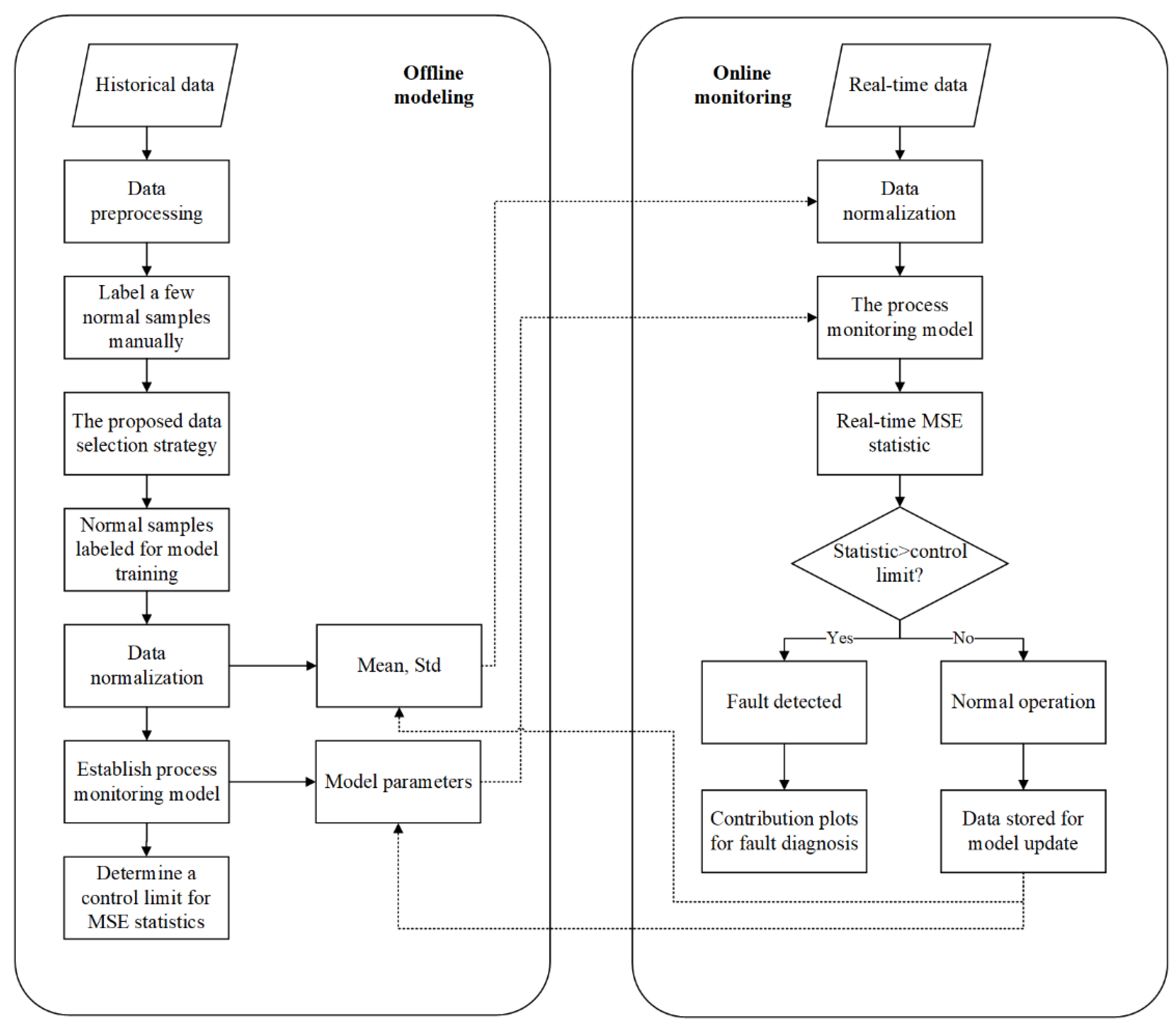
The proposed process monitoring framework can be divided into offline modeling and online monitoring, which can be shown in the flowchart in Figure 2. Details of each part are introduced in this section.

3.1. Information Entropy-Based Data Labeling Strategy with Few Labeled Normal Samples

As mentioned before, sufficient normal training data are an important prerequisite for establishing a process monitoring model. In practice, all the historical data collected from industrial processes are unlabeled. There is inevitably a small number of fault samples in the historical data, which have to be labeled and excluded from the training data. Labeling data manually is almost impossible because of the high labor and time costs. Generally, a few normal samples are first labeled manually, and then a data selection strategy is employed to automatically label normal samples and fault samples from the rest of the historical data. To address this issue, an information entropy-based data selection strategy is proposed and compared to distance-based methods and semi-supervised deep learning methods.

The proposed method aims to automatically label samples according to the dissimilarity measure between the distribution of normal samples and fault samples of key variables using information entropy. The key variables refer to variables that have a great impact on product quality and safety. These variables are usually controlled within a small variation interval, which is hardly influenced by the random disturbances of the process. Therefore, normal process disturbances and real faults can be effectively distinguished by the proposed method.

Given a key variable $x\left(x_1,x_2,\dots ,x_l,\dots ,x_n\right)$, where the first $l$ samples are manually labeled normal samples and $l$ is much less than $n$, the information entropy of normal samples $H\left(x\right)\left[h\left(x_1\right),\dots ,h\left(x_{l-d}\right)\right]$ is first calculated using a sliding window. Details on the selection of window width $d$ are presented in Section 4.2. Since $\left(l-d\right)$ group information entropy has been calculated, a control limit can be calculated as follows to determine the normal variations in the distribution of the variable $x$,

$$h_{limit}=mean\left(h\left(x_1\right),h\left(x_2\right)\dots h\left(x_{l-d}\right)\right)-3 · std\left(h\left(x_1\right),h\left(x_2\right)\dots h\left(x_{l-d}\right)\right)$$

(3)

where$mean\left(\cdot \right)\mathrm{and} std\left(\cdot \right)$ are the average value and standard deviation of the information entropy under normal operating conditions, $h_{limit}$ is the lower control limit. Only the lower control limit is employed because the information entropy will reach its maximum when data are evenly distributed. Therefore, the information entropy remains at a high value for normal samples. When a fault occurs, the distribution of data in the window will change, causing a decrease in its information entropy. Then, the proposed strategy is ready to label samples in the rest of the historical data. The information entropy of unlabeled samples $H\text{'}\left(x\right)[h\left(x_{l-d}\right),\dots ,h\left(x_{n-d}\right)$is calculated and compared with the control limit. New samples whose information entropy is higher than the control limit will be labeled as normal samples; otherwise, they will be labeled as fault samples. After all historical data are labeled, the fault-free samples in historical data are included in the training data to establish the process monitoring model.

The main advantages of the proposed data selection strategy are reflected in two aspects. Firstly, the proposed data selection strategy employs information entropy as the dissimilarity measure between the distribution of key variables in labeled normal samples and unlabeled samples to perform data labeling. The key variables are highly related to product quality or process safety, so they are strictly controlled within a small interval and hardly influenced by random disturbances of the process. Therefore, only real faults that affect the normal process operation can be labeled as fault samples by the proposed method, and the process monitoring model established with training data labeled by the proposed method will show a low false alarm rate and high sensitivity to faults. In contrast, the distance-based methods will be significantly affected by the random disturbances of the process, resulting in situations where the Euclidean distance between normal samples can also be large, even larger than the distance between normal samples and fault samples. In this way, the control limit that represents the normal variations will be large, so that certain fault samples will be labeled as normal samples together with normal process disturbances. Furthermore, the real faults will be buried in these normal process disturbances and cannot be detected by the process monitoring model, making it hard to provide a reliable monitoring result for online applications. Secondly, the proposed data selection strategy does not require a large number of initial labeled samples. The information entropy is a statistical method that can be used to make an accurate estimation of the distribution of data only with proper window width. Therefore, a reliable control limit can be determined with only a few labeled normal samples. This is difficult to implement with semi-supervised deep learning methods. If the initial labeled samples are too limited, it is not able to establish an effective deep learning model since there are a large number of parameters in the model that have to be trained through sufficient training data; otherwise, the model will be overfitting, which will affect the data labeling results, causing a poor generalization ability of the process monitoring model.

3.2. Process Monitoring Modeling

For an industrial process$X\left(m,n\right)$ with $m$ variables and $n$ selected modeling data, a two-layer autoencoder model, which is shown in Figure 1, is trained for feature extraction and fault detection as follows,

$$Z=\sigma \left(W_{1}X+b_1\right)$$

(4)

$$Y=\sigma \left(W_{2}Z+b_2\right)$$

(5)

$$Z^{\prime }=\sigma \left(W_{3}Y+b_3\right)$$

(6)

$$X^{\prime }=\sigma \left(W_4{Z}^{\prime }+b_4\right)$$

(7)

where $Y,Z, Z^{\text{'}}$ are latent variables, $X^{\prime }$ is the construction of $X$, $W_i, b_i$ are weights and bias of the encoder and decoder. The model aims to minimize the reconstruction error between $X$ and $X^{\prime }$. The mean squared error (MSE) is applied in this work, which can be calculated as follows,

$$MSE\left(X,X^{\prime }\right)=\frac{1}{n}{\displaystyle \sum }_{i=1}^n{\left(x_i-x_i^{\text{'}}\right)}^2$$

(8)

where $x_i$ is the sample in $X$, and the $x_i^{\text{'}}$ is the reconstruction of the sample $x_i$. As the autoencoder model has been constructed, modeling data are utilized to train the model, in which two percent of the data are randomly divided as the validation dataset. When the reconstruction error of the training dataset no longer decreases significantly and the error of the validation set reaches a minimum, the model training is completed for real-time monitoring.

3.3. Fault Detection and Diagnosis

To realize real-time fault detection, a monitoring statistic should be constructed to quantify the process operating status. The MSE statistic in Equation (8) is used in this work. The MSE of data under normal operating conditions should be within a threshold, and variable correlation will change significantly when a fault occurs, resulting in a large reconstruction error. Given a series of MSE under normal conditions $MS{E}_{normal}$, the threshold under a 99% confidence interval can be determined through kernel density estimation,

$$\rho \left(MS{E}_{normal}\right)=\frac{1}{n}{\displaystyle \sum }_{i=1}^{n}K\left(MS{E}_{normal}-MS{E}_i\right)$$

(9)

$${{\displaystyle \int }}_{-\infty }^{threshold}\rho \left(MS{E}_{normal}\right)dMS{E}_{normal}=0.99$$

(10)

where $K\left(\cdot \right)$ is the kernel function, which is generally selected as the Gaussian kernel function, $\rho \left(MS{E}_{normal}\right)$ is the probability density function, and $MS{E}_i$ represents the MSE at the $i_{th}$ sample. For real-time monitoring, the MSE statistic is calculated and compared with the threshold. Statistics within the threshold indicate that the system is operated under normal operating conditions, and the data will be stored in the database for the model update. If the statistic exceeds the threshold, a fault is detected and the root cause needs to be isolated immediately. In this work, contribution plots are applied by calculating the contribution rates of each variable to the reconstruction error. The variable with the largest contribution rate is preliminarily diagnosed as the root cause.

3.4. Model Update Strategy

For plant-wide industrial processes, the catalyst activity and equipment structure will change to a certain extent with the increase in operation time, and the operating condition can also be adjusted according to the product price and government regulation. To make the model more applicable to the current operating condition, a model update strategy is also applied in the proposed process monitoring model.

In real-time process monitoring, data that are identified as normal operation by the proposed method are continually saved in the database and supplemented to the modeling data after a period of time for a model update. The model parameters will not change significantly as long as the process is operated under normal conditions. Therefore, the time cost for the model update is negligible and will not affect the application of online monitoring. Moreover, the application of the model update strategy can deal with the multimode issue simultaneously. The multimode issue mostly results from the adjustment of production loads in industrial processes. This kind of mode switching will lead to a step change in the feed flow, which can be easily identified by contribution plots. When the mode switching is identified by the process monitoring model, the model update strategy will start to work, by which the normalization center of the model will be adjusted to the new mode. In most multimode process monitoring methods, all possible modes must be available in the training data. For real-time monitoring, new samples are first clustered into one of the historical modes and then monitored with the corresponding model, which requires an expensive computation cost. More importantly, it is impossible to satisfy the assumption that all modes are included in the training data for an industrial process. By contrast, the proposed process monitoring method employs a model update strategy to make a connection between fault detection and fault diagnosis, by which the multimode issue can be addressed by adjusting the normalization center of the model. The proposed method can be applied to monitor multimode processes even with only one operating mode available in the training data.

In summary, the procedure of the proposed industrial process monitoring framework can be described as follows.

Offline modeling:

(1)

Data are preprocessed to address data deficiency and outliers.

(2)

Fault-free modeling data are automatically selected using the proposed strategy.

(3)

Modeling data are normalized with their average value and standard deviation.

(4)

Modeling data are divided into a training dataset and a validation dataset to train the proposed process monitoring model.

(5)

MSE statistics under normal operating conditions are calculated and the threshold is determined.

Online monitoring:

(1)

Real-time data are normalized with the average value and standard of modeling data.

(2)

Normalized data are put into the process monitoring model for data reconstruction.

(3)

Real-time MSE statistics are calculated using reconstruction errors.

(4)

Real-time MSE statistics are compared with the threshold. Normal data are stored in preparation for model updates, while the fault is diagnosed by contribution plots.

4. Industrial Application of Methanol to Olefin Unit

In this section, the offline modeling and online application of the proposed method on an industrial methanol to olefin unit are introduced.

4.1. Description of the Process and Dataset

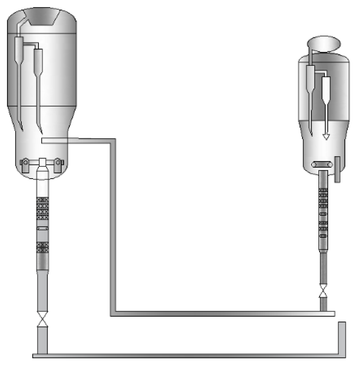
Actual process data collected from the distributed control system of a chemical plant in China are applied for modeling and validation of the proposed model. The flowchart of the core equipment in this methanol to olefin unit is shown in Figure 3, which contains a reactor and regenerator. Data from a one-month period of operation are collected as historical data. The sampling frequency of the data is one minute. A total of 169 process variables in this unit are selected according to the process flow information. Among these variables, the dense-phase temperature of the reactor is a key variable with an obvious impact on product quality. The temperature is controlled within a small range to ensure stable operation. As the temperature decreases, the conversion rate of dimethyl ether will decrease, leading to a decrease in the selectivity of ethylene and propylene. On the other hand, the increase in temperature will aggravate the side reaction rate and increase the carbon deposition rate of the catalyst. Therefore, the dense-phase temperature of the reactor is applied as the key variable of the proposed strategy to automatically select modeling data. Through correlation analysis, 54 variables with a moderate or strong correlation with the dense-phase temperature of the reactor are selected from 169 variables for modeling, which is shown in

Table 1. Variable information of the methanol to olefin unit.

Variable No.	Description
1	Stripping section temperature of reactor
2	Dense-phase temperature of reactor
3	Temperature of reaction gas
4	Standpipe temperature of the catalyst
5	Feed flow of methanol
6	Level of methanol in heat exchanger
…	…
51	Catalyst inventory in stripping section
52	Density of lower stripping section
53	Density of upper stripping section
54	Pressure of catalyst delivery pipe

.

4.2. Data Preprocessing and Selection

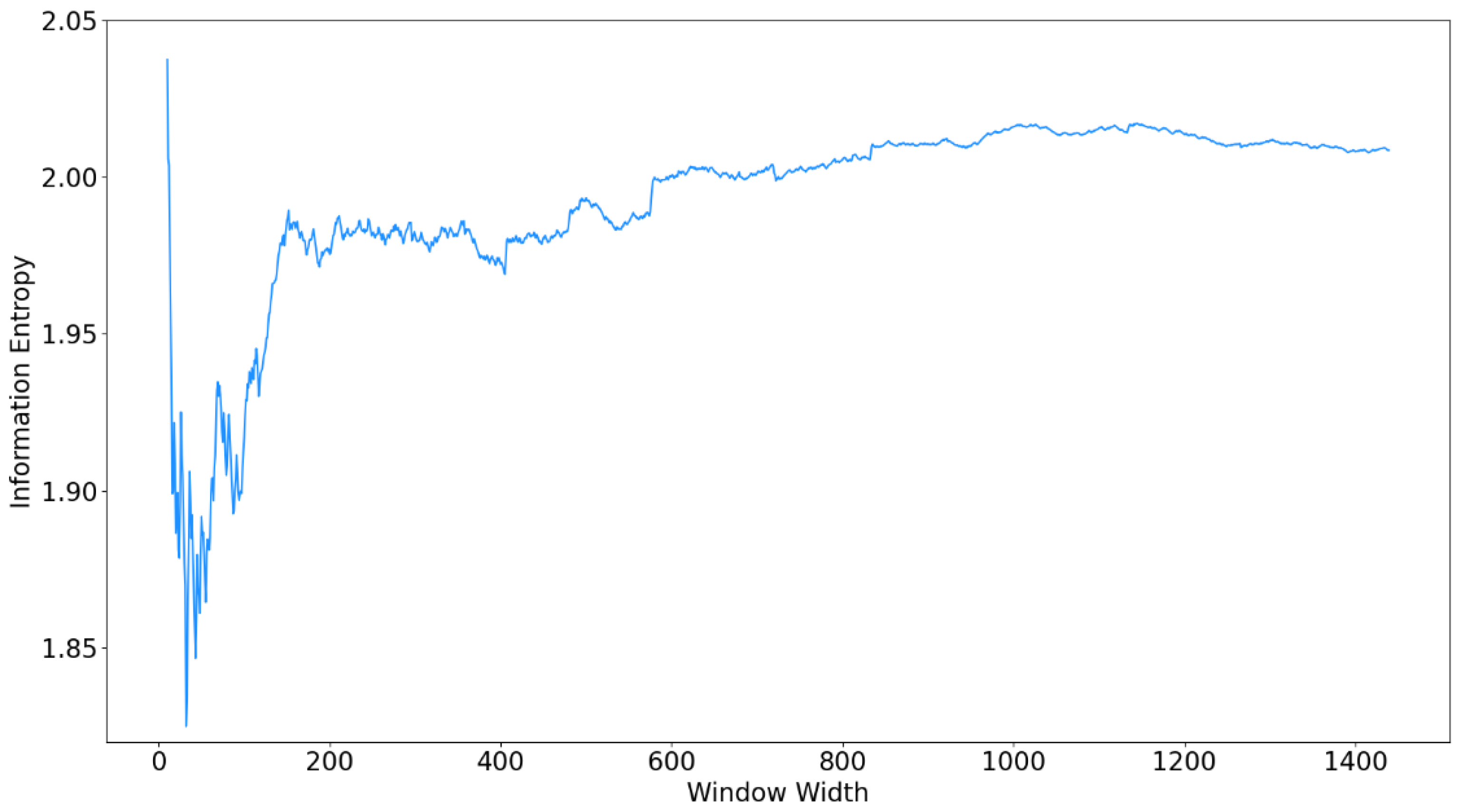
Data preprocessing is first implemented to eliminate samples with data deficiency and outliers. Then, the proposed information entropy-based data selection strategy is employed to label normal samples and fault samples from the historical data. As mentioned before, a small number of normal samples need to be manually labeled in advance. In this work, only 1440 normal samples, which are exact data from a one-day period, are first labeled according to process knowledge and expert experience. To label such a small number of samples does not consume much time or labor costs. On the other hand, it can help demonstrate the effectiveness of the proposed method in data selection with limited labeled normal samples. Before the calculation, a key parameter, the window width, has to be determined. Information entropy does not require a large number of samples to make an accurate estimation of the distribution of data, but a proper window width is required. A too-small window width cannot include sufficient data information for the kernel density estimation calculation, the results will be highly affected by the random part of the data, causing an unreliable information entropy result. As the window width increases, the calculation accuracy will be improved as more data will have been considered. When the data in the sliding windows are sufficient, the information entropy will not change significantly with the increase in the window width, indicating a proper window width has been obtained. To determine the proper window width in this industrial process, an experiment is implemented using the labeled 1440 normal samples in Figure 4. The information entropy of the dense-phase temperature of the reactor is calculated sequentially when the window width is between 10 and 1440. As expected, when the window width is small, the information entropy varies greatly with the window width. The calculation is unreliable when the window width is too small until when the window width reaches 180 min; the information entropy will not change significantly with the increase in the window width. Therefore, 180 is selected as the window width in this study.

It can be concluded from Figure 4 that it does not require too many samples to estimate the distribution of data using information entropy. Moreover, excessive window width is also unacceptable. On the one hand, the calculation accuracy can hardly be further improved. On the other hand, excessive window width will result in the low sensitivity of the method to identify fault samples in labeling historical data. In addition, the key variable is strictly controlled in a small interval during normal operations. The data distribution is similar under normal operations. Information entropy, as a statistical algorithm to measure the distribution of data, can be applied to determine the control limit for the normal variations in the distribution of the key variable with only a few labeled normal samples. Unlike deep learning models, which require massive samples to train a large number of model parameters, the proposed data selection strategy is more applicable to practical applications.

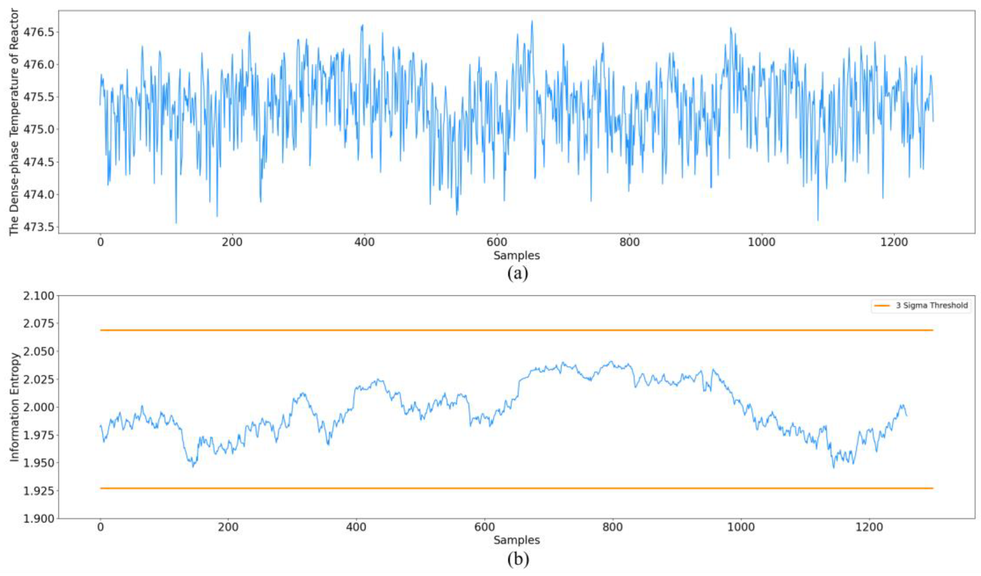
As the window width has been determined, the distribution of the dense-phase temperature of the reactor under normal conditions can be estimated by the information entropy with a sliding window. With 1440 labeled normal samples and a window width of 180, 1260 sets of information entropy can be calculated, which is shown in Figure 5. The subgraph on the top is the initial labeled normal data of the dense-phase temperature of the reactor. The corresponding information entropy is shown in the subgraph at the bottom. It can be seen that the variable operated under normal conditions with small fluctuations, and accordingly, the information entropy is close to each other in different samples. The small dissimilarity between the distribution of normal samples results from random factors during normal process operations and can be reflected in the calculation value of information entropy. A three-sigma control limit for the normal variations is then determined, which can be shown in Figure 5. As discussed before, the lower threshold is used because the fault will lead to a decrease in the information entropy.

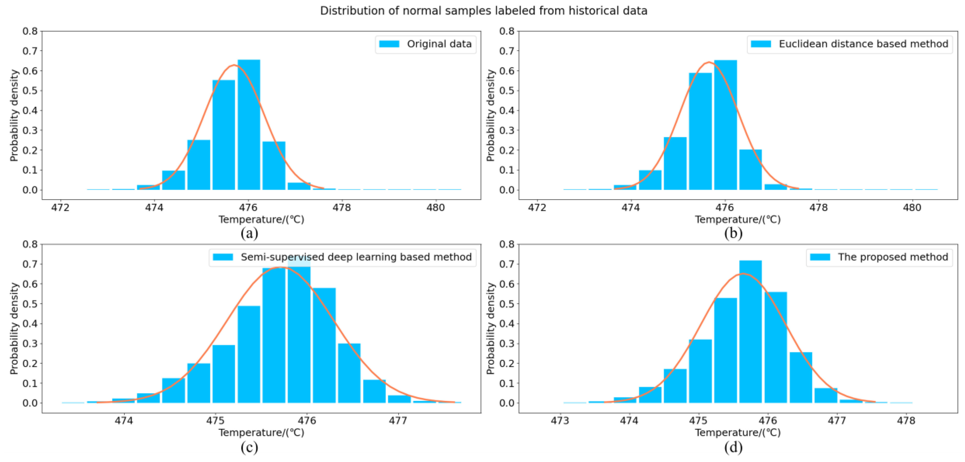
After the window width and the threshold have been determined, normal samples and fault samples in the unlabeled historical data can be automatically labeled by calculating information entropy and comparing them with the control limit. There are 43,200 historical samples to be labeled, and the samples whose information entropy is within the control limit are retained as training data of the process monitoring model. In contrast, the samples whose information entropy is outside the control limit are labeled as fault samples and excluded. The results are compared with original data, Euclidean distance-based data labeling method, and a semi-supervised deep learning-based method. As shown in Figure 6, the data labeling performance of different methods is displayed through the distribution of the labeled normal samples.

Although the original data approximately conforms to the normal distribution, obviously there are a few fault samples in the historical dataset. This small proportion of fault samples has to be excluded from the training data; otherwise, the fault in practical production will not be effectively detected by the process monitoring model. The distribution of normal data labeled by the Euclidean distance-based method is similar to the original data. As discussed before, the Euclidean distance is highly affected by random process disturbances, and cannot be applied as an effective dissimilarity measure. According to statistics, 86 percent of the historical data are labeled as the training data, while it can be observed in Figure 6 that fault samples are included in the training data, and therefore the real faults cannot be detected by the process monitoring model in the online application. The normal data labeled by the semi-supervised deep learning method conform to a normal distribution, and fault samples have been effectively excluded from the historical data. However, it is worth noting that only 59 percent of the historical data remain, which means that a large number of normal samples may be labeled as fault samples. The reason lies in the poor generalization ability of the deep learning model. As mentioned before, there are a large number of parameters to be trained with sufficient labeled samples. Although more labels can be automatically obtained through semi-supervised learning, the lack of initial labeled samples still limits their application in complex industrial processes. The samples labeled from historical data are all normal samples, but they are not enough to represent all normal behaviors of the process, which will result in massive false alarm rates in real-time monitoring. By comparison, the proposed method shows the best performance. The distribution of the training data labeled by the proposed method is closest to a normal distribution; 82 percent of the historical data have been labeled as normal samples, which is 23 percent more than the semi-supervised deep learning-based method. The results illustrate that the proposed data selection strategy can effectively distinguish between normal and faulty samples from massive unlabeled historical data with only a few labeled normal samples. With the proposed method, a reliable historical dataset can be obtained, which can significantly benefit the process monitoring performance. The process monitoring results will be compared and discussed in the next section.

4.3. Process Monitoring Modeling and Result Analysis

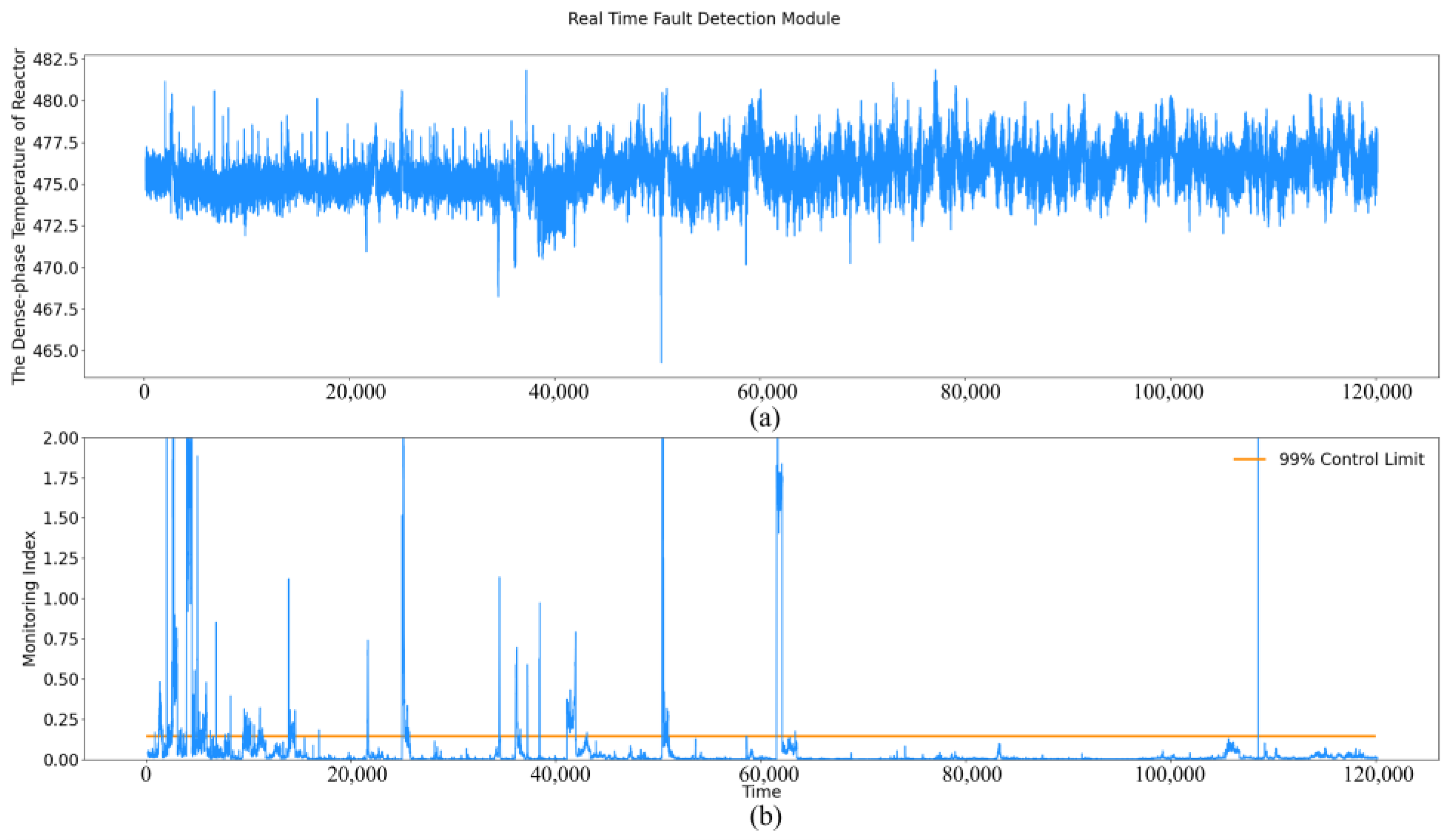
As the training data labeled by the proposed data selection strategy and other methods have been obtained, a two-layer autoencoder is constructed and trained to further compare the online process monitoring performance of different methods. For a fair comparison, all process monitoring methods are set to the same model structure, hyperparameters, and model update strategies. In this work, the number of hidden layer units is selected as 128, and the activation function is the tanh function. The training data labeled by each method are input into the corresponding model in batches with a window length of 10, and two percent of modeling data are randomly selected as the validation dataset. When the model training has been completed, it is applied for online monitoring. Both normal samples and faulty samples are recorded in real-time operation. The root cause of the faults is diagnosed online and saved in a historical fault database, while normal data is saved together with modeling data for the model update. The results of a three-month online application of the proposed method are shown in Figure 7.

As expected, the proportion of faults is quite small compared to normal operations, and it can be preliminarily observed that most alarms correspond to abnormal deviations in the dense-phase temperature of the reactor. For computational loads, the calculation speed of this model is fast enough for online monitoring because the complexity of the model is not very high. Each monitoring result can be given within one second, which is far less than the sampling frequency. In addition, there are multiple operating modes during these three-month process operations, which have also been effectively addressed by the proposed process monitoring framework through the model update strategy. As shown in

Table 2. Calculation time of each model update.

Update No.	Time
1	52.43
2	11.06
3	18.69
4	8.33
5	3.64
6	12.46
…	…
80	8.12
81	3.00
82	21.23
Average	14.44

, the calculation speed will be slower when the model is updated online, but also within the acceptable range. Most importantly, most alarms on abnormal deviations can be given by the proposed model in advance of what can be observed, which means that operators can take corresponding measures in advance to avoid these faults according to the results provided by the proposed model. The above conclusions will be specifically proved and analyzed below through several fault cases.

The process monitoring results were also calculated using training data labeled by the Euclidean distance-based method and the semi-supervised deep learning-based method for comparison. The results shown in Figure 8 are obtained from the model trained with data labeled by the Euclidean distance-based method. It can be found that the alarms of this method are much less than the proposed method. As discussed in the last section, the training data labeled by the Euclidean distance include fault samples, which leads to a wider control limit for normal variations. As a result, the control limit of the MSE statistic is determined as 0.145, which is much higher than that of the proposed method, 0.067. It indicates that the interval determined for the normal variations is much wider. Therefore, there could be many fault samples with a minor magnitude that cannot be detected. That is the reason why there are fewer alarms triggered by the model in Figure 8 than in the proposed method. The process monitoring results obtained from the model trained with data labeled by the semi-supervised deep learning-based method are shown in Figure 9. The limited initial labeled samples result in a poor generalization ability of the deep learning model, so only a small part of normal samples can be labeled from historical data, which cannot represent all the normal behaviors of the process. Therefore, the process monitoring model established using insufficient historical data only works well in test data that are close to the training data. As time goes on, massive false alarms will be triggered in new test data, which can be shown in Figure 9. It is difficult to distinguish real faults from false alarms according to the process monitoring results, making it not applicable for practical application. Through comparison, the proposed process monitoring framework shows better performance in the long-term monitoring of industrial processes, which is consistent with the analysis of the data labeling results in the last section. Next, the process monitoring performance will be further analyzed through several specific fault cases detected by the proposed method.

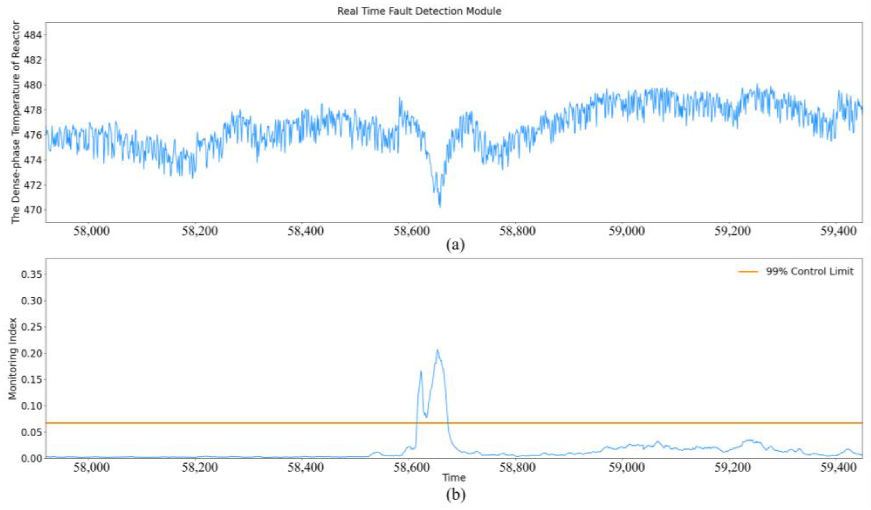
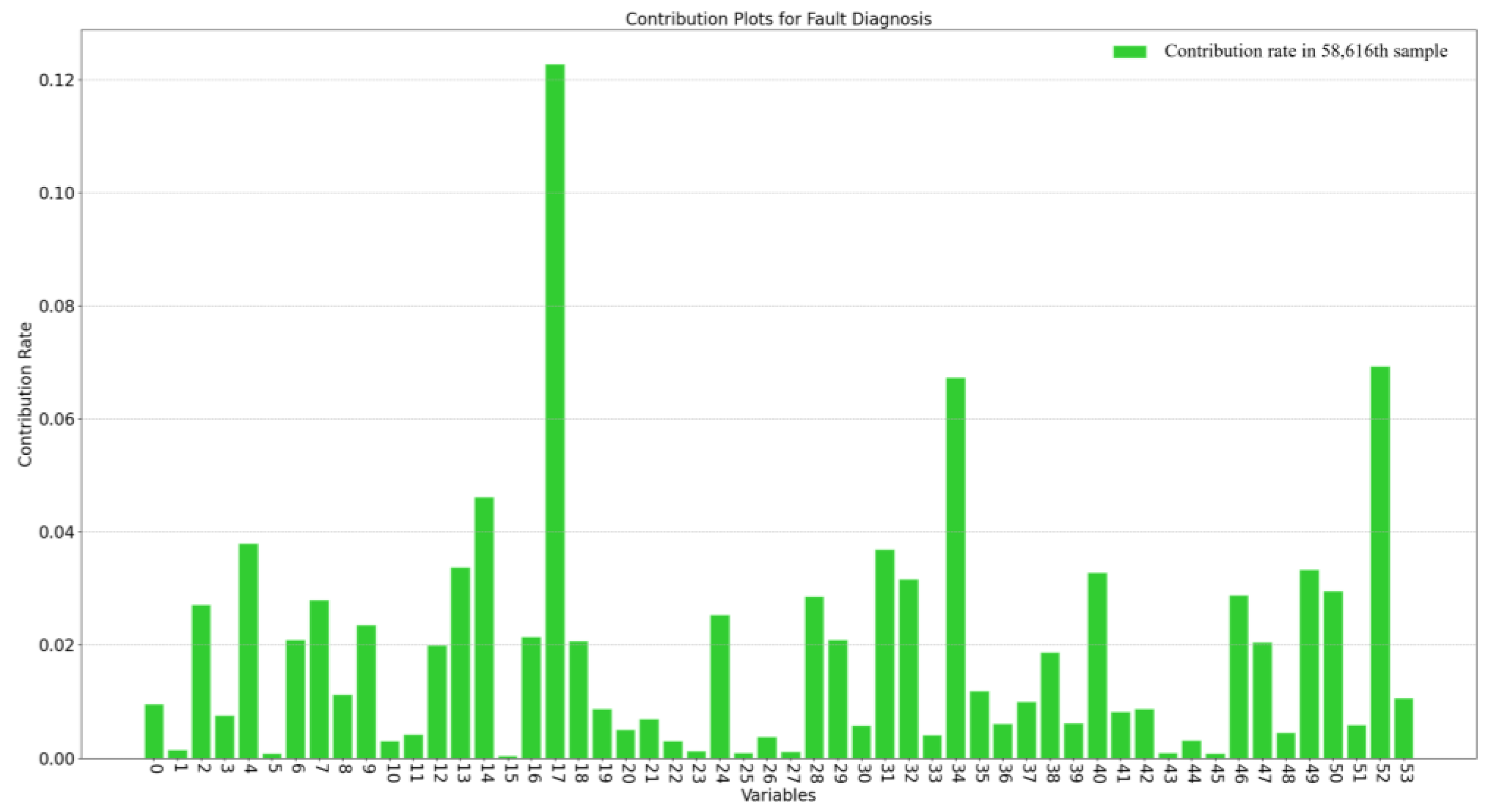
The process monitoring result of the first case is shown in Figure 10. The reconstruction error continuously increased and exceeded the threshold at the 58,616th sample. It can be observed from the original data that an abnormal deviation of about six degrees Celsius occurs in the dense-phase temperature of the reactor. The point is that the abnormal deviation cannot be observed from the original data of the dense-phase temperature of the reactor until about forty minutes after the alarm was given by the proposed model. According to the contribution plots in Figure 11, the steam flow rate in the upper stripping section of the reactor is with the highest contribution rate, and is diagnosed as the root cause. The results can be validated from the original data that there is a significant step drop in the steam flow. Given the results from the screen, the operators have sufficient time to inspect the steam valve and take appropriate measures to avoid this abnormal deviation in temperature.

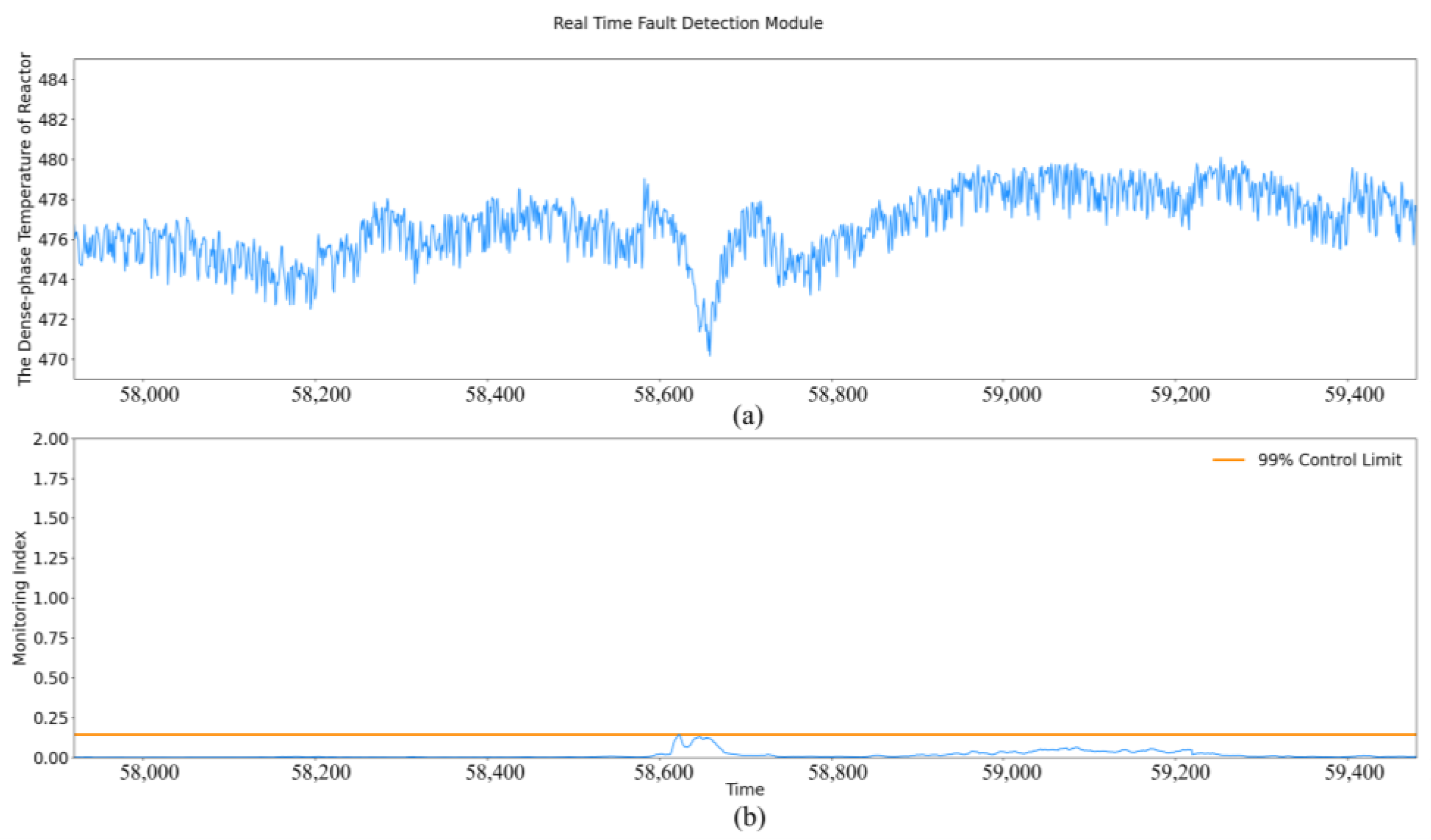
The process monitoring results of other methods on this fault are also used for comparison. The result of the model with data labeled by the semi-supervised deep learning-based method does not need to be displayed, as the process monitoring results are almost all false alarms, which are not reliable for practical application. The result of the model with data labeled by the Euclidean distance-based method is displayed in Figure 12. It can be shown that the fault is barely detected by the process monitoring model. The results support the previous conclusion that although there are fewer alarms in the process monitoring model using the Euclidean distance-based data labeling strategy, the sensitivity of the model to real faults is reduced. A similar conclusion can be obtained in other cases, so the following fault cases will focus on the analysis of process monitoring results provided by the proposed method.

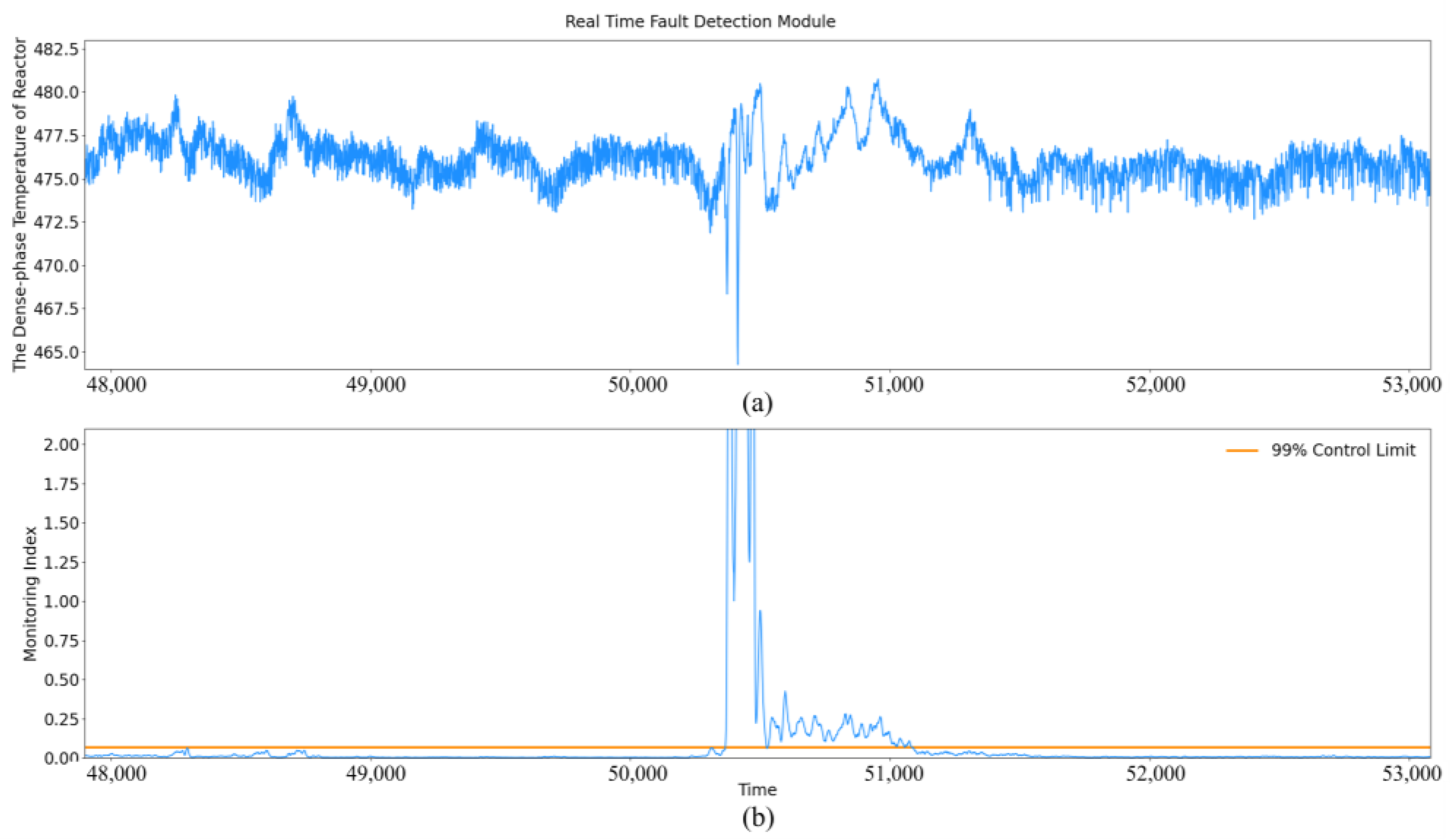
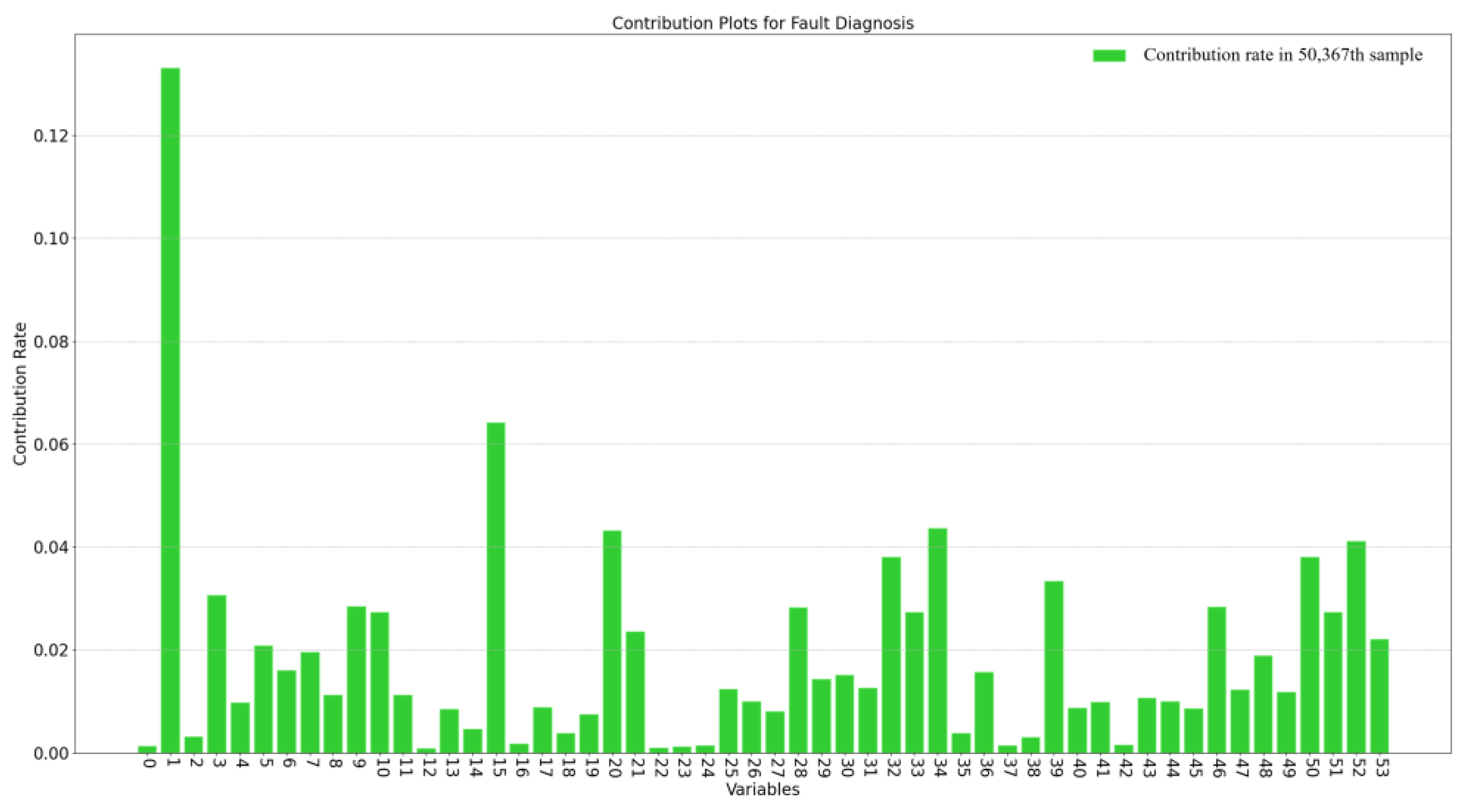
For the second case shown in Figure 13, a fault is detected at the 50,367th sample. According to the original data, an abnormal deviation lasting a thousand minutes occurs in the dense-phase temperature of the reactor about five minutes after the alarm was given by the proposed model. The faults cannot be detected by distributed control system because the measured value does not reach the high or low alarm limit, but such long periods of fluctuation can lead to changes in product quality and therefore need to be detected early. The contribution plots in Figure 14 show that the variable with the highest contribution rate is the dense-phase temperature of the reactor. Therefore, the fault may be caused by changes in feed composition or equipment structure, which have not been measured in historical data. Although the root cause is not directly determined, the proposed method still provides the operators enough time to take action to avoid this fault.

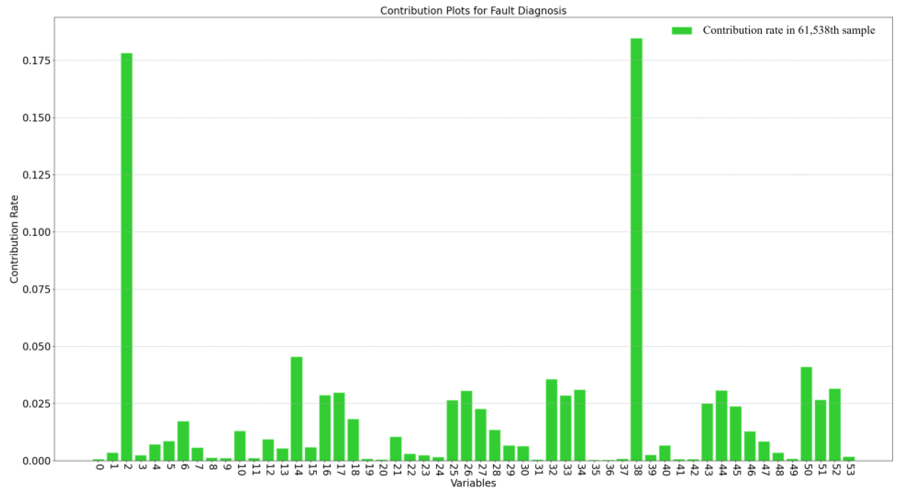
For the next case shown in Figure 15, a fault was detected by the proposed process monitoring method at the 61,538th sample. Although only three degrees Celsius deviation in the dense-phase temperature of the reactor is caused, the monitoring statistic still exceeds the threshold. It can be concluded from the fault diagnosis result in Figure 16 that the temperature of the reaction gas is the root cause of this fault. According to the original data, a step deviation occurs in the temperature of reaction gas during this model alarm. Although this deviation does not have an obvious impact on the dense-phase temperature of the reactor, it still should be alerted to the operators.

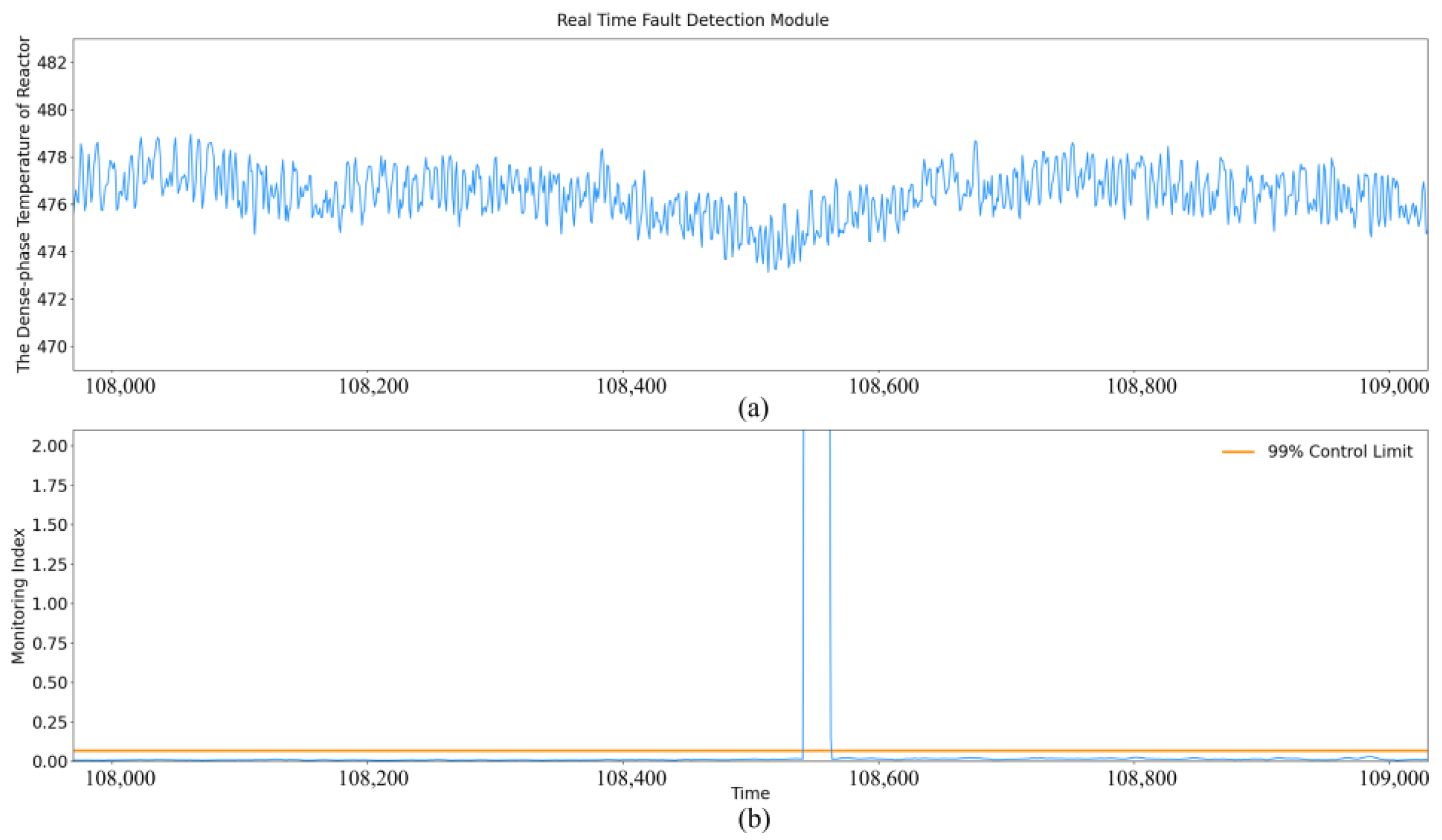
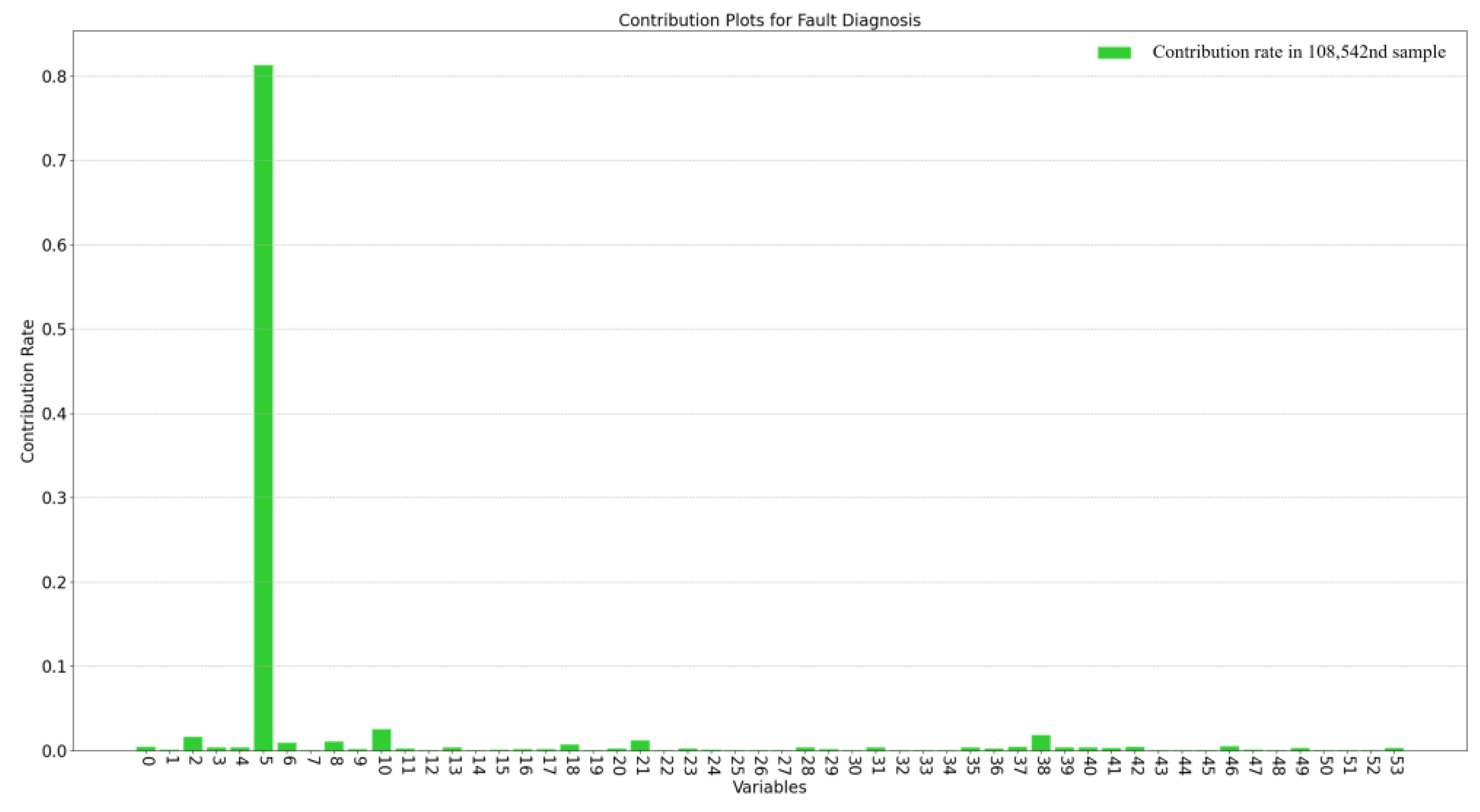
Finally, there are also many different operating modes during the three-month process operations. The last case will display the process monitoring results of the proposed method when the operating mode is adjusted. As shown in Figure 17, the monitoring statistics of a few samples exceed the threshold at about the 108,540th sample, but the reactor temperature has not been affected. The alarm is triggered and the fault diagnosis model starts to work. As shown in Figure 18, only one variable shows an obvious significant contribution to this fault, which is the feed flow rate. The results show that the alarms are triggered because of the switch of operating modes, as the production load needs to be adjusted. Although a few false alarms are triggered, the fault diagnosis results are immediately provided to operators that the operating mode has been adjusted, and the model will be quickly updated to the new mode, by which the alarms are removed. Overall, the analysis of the above cases shows that the proposed method has a long-term effective performance in large-scale industrial process monitoring.

5. Conclusions

In this work, we propose a new automatic selection strategy for modeling data of industrial process monitoring based on information entropy. Compared to expert knowledge-based, distance-based, and semi-supervised deep learning-based data selection strategies, the proposed strategy requires lower labor costs, and is more applicable to industrial processes with limited labeled normal samples. Based on this strategy, a data-driven process monitoring framework is developed and a model update strategy is employed to make a connection between fault detection and fault diagnosis for addressing the multimode issue.

The proposed process monitoring framework is applied to a large-scale industrial methanol to olefin unit of a practical chemical plant in China. The results show that the normal samples and fault samples can be correctly labeled by the proposed data selection strategy with only 1440 manually labeled normal samples. A long-term effective process monitoring model is then established based on all normal samples labeled from historical data. The process monitoring performance of the model has been tested in an approximately three-month online application. The results indicate that faults can be detected earlier by the proposed method than by operators through observation, and the root cause of the faults can be preliminarily diagnosed as well. The real-time process monitoring results can be delivered to operators in practical operation, by which they could take action to minimize the impact of faults. Details of the proposed data selection strategy and modeling process have also been provided to demonstrate the replicability, by which we hope to provide a certain reference for other researchers or companies, thereby facilitating a wider industrial application of process monitoring systems.

Although data-driven process monitoring has made great progress, there are several considerations for its practical application. The training data must be large enough to represent various normal behaviors of the process; otherwise, frequent false alarms will be triggered. For example, there are slow changes over time in chemical processes, such as equipment aging and catalyst deactivation. Generally, these changes can be regarded as normal situations in process operation. They have to be considered in establishing the process monitoring model to avoid false alarms. In addition, fault samples should not be included in the training data; otherwise, the faults will be difficult to be detected by the process monitoring model. Therefore, an effective data labeling strategy is required to address the above issues. Another important consideration is the selection of the process monitoring model and parameters. The model is established aiming to extract features from the training data and determine a control limit for normal variations using a statistic. The model should be selected according to the data characteristics of the target process. For example, the industrial process investigated in this work is highly nonlinear with complex variable relationships, which is hard to be captured by multivariate statistical methods. At the same time, there are sufficient historical data available to establish a deep learning model with great generalization ability. Therefore, a multi-layer autoencoder is employed in this work. Moreover, several model parameters have to be determined no matter which model is employed, such as the number of principal components in PCA and the structure of deep learning models. The identification of optimal model parameters is an important research issue to be discussed, which can be referred to in many existing studies.

Through the above considerations, the proposed process monitoring framework has achieved a promising performance through a three-month test in an industrial process, but there are still several limitations. The fault is localized at the variable with the highest contribution rate in this work, while it is difficult to determine the root cause if the fault has been propagated among process variables. Under this circumstance, there will be more variables with a high contribution rate and the variable with the highest contribution rate may not be the root cause of the fault. Another limitation is that the model update strategy may not be sufficient for more complex scenarios. The proposed method addresses the multimode issue through a model update strategy, as the variable correlation will not obviously change in different operating modes. However, the previous model may no longer be applicable after the replacement of the catalyst or shut-down maintenance because the variable correlation has changed. The model has to be re-trained with new data rather than just updating the model parameters. Therefore, future work will lie in the improvement of the process monitoring framework according to the considerations and limitations mentioned above.

References

1. Severson, K.; Chaiwatanodom, P.; Braatz, R.D. Perspectives on process monitoring of industrial systems. Annu. Rev. Control 2016, 42, 190–200. [Google Scholar] [CrossRef]
2. Frank, P.M. Fault diagnosis in dynamic systems using analytical and knowledge-based redundancy: A survey and some new results. Automatica 1990, 26, 459–474. [Google Scholar] [CrossRef]
3. Venkatasubramanian, V.; Rengaswamy, R.; Kavuri, S.N.; Yin, K. A review of process fault detection and diagnosis Part III: Process history based methods. Comput. Chem. Eng. 2003, 27, 327–346. [Google Scholar] [CrossRef]
4. Qin, S.J. Survey on data-driven industrial process monitoring and diagnosis. Annu. Rev. Control 2012, 36, 220–234. [Google Scholar] [CrossRef]
5. Ge, Z.; Song, Z.; Gao, F. Review of Recent Research on Data-Based Process Monitoring. Ind. Eng. Chem. Res. 2013, 52, 3543–3562. [Google Scholar] [CrossRef]
6. Ge, Z. Review on data-driven modeling and monitoring for plant-wide industrial processes. Chemom. Intell. Lab. Syst. 2017, 171, 16–25. [Google Scholar] [CrossRef]
7. Reis, M.; Gins, G. Industrial Process Monitoring in the Big Data/Industry 4.0 Era: From Detection, to Diagnosis, to Prognosis. Processes 2017, 5, 35. [Google Scholar] [CrossRef] [Green Version]
8. Kresta, J.V.; MacGregor, J.F.; Marlin, T.E. Multivariate statistical monitoring of process operating performance. Can. J. Chem. Eng. 1991, 69, 35–47. [Google Scholar] [CrossRef]
9. Negiz, A.; Çinar, A. Statistical monitoring of multivariable dynamic processes with state-space models. AlChE J. 1997, 43, 2002–2020. [Google Scholar] [CrossRef]
10. Kano, M.; Tanaka, S.; Hasebe, S.; Hashimoto, I.; Ohno, H. Monitoring independent components for fault detection. AlChE J. 2003, 49, 969–976. [Google Scholar] [CrossRef]
11. Schölkopf, B.; Smola, A.; Müller, K.-R. Nonlinear component analysis as a kernel eigenvalue problem. Neural Comput. 1998, 10, 1299–1319. [Google Scholar] [CrossRef] [Green Version]
12. Apsemidis, A.; Psarakis, S.; Moguerza, J.M. A review of machine learning kernel methods in statistical process monitoring. Comput. Ind. Eng. 2020, 142, 106376. [Google Scholar] [CrossRef]
13. Ku, W.; Storer, R.H.; Georgakis, C. Disturbance detection and isolation by dynamic principal component analysis. Chemom. Intell. Lab. Syst. 1995, 30, 179–196. [Google Scholar] [CrossRef]
14. Li, G.; Liu, B.; Qin, S.J.; Zhou, D. Dynamic latent variable modeling for statistical process monitoring. IFAC Proc. Vol. 2011, 44, 12886–12891. [Google Scholar] [CrossRef]
15. Dong, Y.; Qin, S.J. A novel dynamic PCA algorithm for dynamic data modeling and process monitoring. J. Process Control. 2018, 67, 1–11. [Google Scholar] [CrossRef]
16. Zheng, J.; Zhao, C.; Gao, F. Retrospective comparison of several typical linear dynamic latent variable models for industrial process monitoring. Comput. Chem. Eng. 2022, 157, 107587. [Google Scholar] [CrossRef]
17. Hinton, G.E.; Salakhutdinov, R.R. Reducing the dimensionality of data with neural networks. Science 2006, 313, 504–507. [Google Scholar] [CrossRef] [Green Version]
18. Sakurada, M.; Yairi, T. Anomaly Detection Using Autoencoders with Nonlinear Dimensionality Reduction. In Proceedings of the MLSDA 2014 2nd Workshop on Machine Learning for Sensory Data Analysis—MLSDA’14, Gold Coast, Australia, 2 December 2014; pp. 4–11. [Google Scholar]
19. Fan, J.; Wang, W.; Zhang, H. AutoEncoder based high-dimensional data fault detection system. In Proceedings of the 2017 IEEE 15th international conference on industrial informatics (indin), Emden, Germany, 24–26 July 2017; pp. 1001–1006. [Google Scholar]
20. Wan, F.; Guo, G.; Zhang, C.; Guo, Q.; Liu, J. Outlier Detection for Monitoring Data Using Stacked Autoencoder. IEEE Access 2019, 7, 173827–173837. [Google Scholar] [CrossRef]
21. Zheng, S.; Zhao, J. A new unsupervised data mining method based on the stacked autoencoder for chemical process fault diagnosis. Comput. Chem. Eng. 2020, 135, 106755. [Google Scholar] [CrossRef]
22. Yu, W.; Zhao, C. Robust Monitoring and Fault Isolation of Nonlinear Industrial Processes Using Denoising Autoencoder and Elastic Net. IEEE Trans. Control. Syst. Technol. 2020, 28, 1083–1091. [Google Scholar] [CrossRef]
23. Kingma, D.P.; Welling, M. Auto-encoding variational bayes. arXiv 2013, arXiv:1312.6114. [Google Scholar]
24. Cheng, F.; He, Q.P.; Zhao, J. A novel process monitoring approach based on variational recurrent autoencoder. Comput. Chem. Eng. 2019, 129, 106515. [Google Scholar] [CrossRef]
25. Zhang, S.; Qiu, T. A dynamic-inner convolutional autoencoder for process monitoring. Comput. Chem. Eng. 2022, 158, 107654. [Google Scholar] [CrossRef]
26. Qian, M.; Li, Y.-F.; Han, T. Positive-Unlabeled Learning-Based Hybrid Deep Network for Intelligent Fault Detection. IEEE Trans. Ind. Inform. 2022, 18, 4510–4519. [Google Scholar] [CrossRef]
27. Ji, C.; Sun, W. A Review on Data-Driven Process Monitoring Methods: Characterization and Mining of Industrial Data. Processes 2022, 10, 335. [Google Scholar] [CrossRef]
28. Zhao, C.; Huang, B. A full-condition monitoring method for nonstationary dynamic chemical processes with cointegration and slow feature analysis. AlChE J. 2017, 64, 1662–1681. [Google Scholar] [CrossRef]
29. Jiang, Q.; Yan, X.; Huang, B. Review and Perspectives of Data-Driven Distributed Monitoring for Industrial Plant-Wide Processes. Ind. Eng. Chem. Res. 2019, 58, 12899–12912. [Google Scholar] [CrossRef]
30. Quiñones-Grueiro, M.; Prieto-Moreno, A.; Verde, C.; Llanes-Santiago, O. Data-driven monitoring of multimode continuous processes: A review. Chemom. Intell. Lab. Syst. 2019, 189, 56–71. [Google Scholar] [CrossRef]
31. Wu, H.; Zhao, J. Self-adaptive deep learning for multimode process monitoring. Comput. Chem. Eng. 2020, 141, 107024. [Google Scholar] [CrossRef]
32. Kwak, S.; Ma, Y.; Huang, B. Extracting nonstationary features for process data analytics and application in fouling detection. Comput. Chem. Eng. 2020, 135, 106762. [Google Scholar] [CrossRef]
33. Potočnik, P.; Govekar, E. Semi-supervised vibration-based classification and condition monitoring of compressors. Mech. Syst. Signal Process. 2017, 93, 51–65. [Google Scholar] [CrossRef] [Green Version]
34. Bekker, J.; Davis, J. Learning from positive and unlabeled data: A survey. Mach. Learn. 2020, 109, 719–760. [Google Scholar] [CrossRef] [Green Version]
35. Zheng, S.; Zhao, J. High-fidelity positive-unlabeled deep learning for semi-supervised fault detection of chemical processes. Process Saf. Environ. Prot. 2022, 165, 191–204. [Google Scholar] [CrossRef]
36. Mistry, P.; Lane, P.; Allen, P. Railway Point-Operating Machine Fault Detection Using Unlabeled Signaling Sensor Data. Sensors 2020, 20, 2692. [Google Scholar] [CrossRef] [PubMed]
37. Fan, C.; Liu, Y.; Liu, X.; Sun, Y.; Wang, J. A study on semi-supervised learning in enhancing performance of AHU unseen fault detection with limited labeled data. Sustain. Cities Soc. 2021, 70, 102874. [Google Scholar] [CrossRef]
38. Li, T.; Fan, W.; Luo, Y. A method on selecting reliable samples based on fuzziness in positive and unlabeled learning. arXiv 2019. [Google Scholar] [CrossRef]
39. He, Q.P.; Wang, J. Fault Detection Using the k-Nearest Neighbor Rule for Semiconductor Manufacturing Processes. IEEE Trans. Semicond. Manuf. 2007, 20, 345–354. [Google Scholar] [CrossRef]
40. Gao, X.; Yang, F.; Feng, E. A process fault diagnosis method using multi-time scale dynamic feature extraction based on convolutional neural network. Can. J. Chem. Eng. 2020, 98, 1280–1292. [Google Scholar] [CrossRef]
41. Hu, H.; Sha, C.; Wang, X.; Zhou, A. A unified framework for semi-supervised PU learning. World Wide Web 2013, 17, 493–510. [Google Scholar] [CrossRef]
42. Zheng, S.; Zhao, J. A Self-Adaptive Temporal-Spatial Self-Training Algorithm for Semi-Supervised Fault Diagnosis of Industrial Processes. IEEE Trans. Ind. Inform. 2021, 18, 6700–6711. [Google Scholar] [CrossRef]
43. Wang, X.; Feng, H.; Fan, Y. Fault detection and classification for complex processes using semi-supervised learning algorithm. Chemom. Intell. Lab. Syst. 2015, 149, 24–32. [Google Scholar] [CrossRef]
44. Kumar, A.; Bhattacharya, A.; Flores-Cerrillo, J. Data-driven process monitoring and fault analysis of reformer units in hydrogen plants: Industrial application and perspectives. Comput. Chem. Eng. 2020, 136, 106756. [Google Scholar] [CrossRef]
45. Shannon, C.E. A mathematical theory of communication. Bell Syst. Tech. J. 1948, 27, 379–423. [Google Scholar] [CrossRef] [Green Version]
46. Silverman, B.W. Density Estimation for Statistics and Data Analysis; Chapman & Hall: London, UK, 1986. [Google Scholar]
Figure 1. The structure of the autoencoder used in this work.
Processes 11 00402 g001
Figure 2. The flowchart of the proposed industrial process monitoring framework.
Processes 11 00402 g002
Figure 3. The methanol to olefin unit of an actual chemical plant in China.
Processes 11 00402 g003
Figure 4. The information entropy calculated with different window widths.
Processes 11 00402 g004
Figure 5. Initial manually labeled normal samples and their information entropy: (a) original labeled normal samples; (b) information entropy of these normal samples.
Processes 11 00402 g005
Figure 6. Comparison results on the data labeling performance of different methods: (a) original data; (b) Euclidean distance-based method; (c) semi-supervised deep learning-based method; (d) the proposed method.
Processes 11 00402 g006
Figure 7. Three-month online process monitoring results (the model is trained with data labeled by the proposed method): (a) Original data of the key variable; (b) Fault detection results.
Processes 11 00402 g007
Figure 8. Three-month online process monitoring results (the model is trained with data labeled by the Euclidean distance-based method): (a) Original data of the key variable; (b) Fault detection results.
Processes 11 00402 g008
Figure 9. Three-month online process monitoring results (the model is trained with data labeled by semi-supervised deep learning-based method): (a) Original data of the key variable; (b) Fault detection results.
Processes 11 00402 g009
Figure 10. Process monitoring result on case one obtained by the proposed method: (a) Original data of the key variable; (b) Fault detection results.
Processes 11 00402 g010
Figure 11. Contribution plots calculated in 58,616th sample.
Processes 11 00402 g011
Figure 12. Process monitoring result on case one obtained by the model using Euclidean distance-based data labeling strategy: (a) Original data of the key variable; (b) Fault detection results.
Processes 11 00402 g012
Figure 13. Process monitoring result of the proposed method on case two: (a) Original data of the key variable; (b) Fault detection results.
Processes 11 00402 g013
Figure 14. Contribution plots calculated in 50,367th sample.
Processes 11 00402 g014
Figure 15. Process monitoring result of the proposed method on case three: (a) Original data of the key variable; (b) Fault detection results.
Processes 11 00402 g015
Figure 16. Contribution plots calculated in 61,538th sample.
Processes 11 00402 g016
Figure 17. Process monitoring result when the operating mode is adjusted: (a) Original data of the key variable; (b) Fault detection results.
Processes 11 00402 g017
Figure 18. Contribution plots calculated in the 108,542nd sample.
Processes 11 00402 g018