CFD Modeling and Validation of Blast Furnace Gas/Natural Gas Mixture Combustion in an Experimental Industrial Furnace

Abstract

The use of residual gases from steel production processes as fuel for steel treatment furnaces has attracted great interest as a method for reducing fossil fuel consumption and the steel footprint. However, these gases often have a low calorific value, and a direct substitution can lead to low temperatures or combustion instability issues. CFD simulations of the combustion of these gases can help steel producers forecast the results of the substitution before real testing and implementation. In this study, a CFD model of an industrial experimental furnace in the steel sector is developed and validated. The results are calculated using the combustion, radiation, and heat transfer models included in the software Ansys Fluent. The validation of the simulated results is performed with data acquired from experimental tests under the same simulated conditions at three air-to-fuel equivalence ratios, which vary from an excess of 0% to an excess of 5% oxygen at the outlet. The model is adjusted to the results, capturing the trends of the measured physical variables and pollutant concentrations. In the case of the combustion temperature, the differences between the simulated and measured values vary from 0.03% to 6.9. Based on the simulation results, the use of blast furnace gas as fuel produces temperatures inside the chamber between 1004 °C and 1075 °C and high stream velocities because of the high flow needed to keep the power constant. Flames exhibit straight movements since the high flows absorb the effect of the swirling flames. The addition of natural gases increases the combustion temperature up to 1211 °C and reduces the flow and length of the flames. Finally, temperatures up to 1298 °C and shorter flames are reached with natural gas enriched with a stream of oxygen, but in this case, NOx emissions need to be controlled.

1. Introduction

The current energy scenario has boosted the use of efficient and sustainable alternatives for energy generation and pollutant emission mitigation in intensive industries. In recent years, waste heat recovery [1], waste stream valorization as fuels [2], and electrical flexibility [3] have been presented as promising alternatives for improving the efficiency of production processes.

In particular, the iron and steel industries, which contribute 8% of the overall CO₂ emissions generated by humans, are the sectors more involved in the application of these measures, with the goal of obtaining not only environmental but also economic benefits because of the savings in the emissions of greenhouse gases [4].

Steel producers who use traditional, basic oxygen steelmaking processes use molten iron from blast furnaces as raw materials. Within blast furnaces, coke, iron ore, and lime are subjected to a reduction process that generates a CO-rich gas, known as blast furnace gas (BFG), as a byproduct of the internal chemical reactions. BFG has a composition that varies depending on the steel plant’s location, but it usually contains about 20–30% CO, 2–6% H₂, 45–60% N₂, and 20–25% CO₂ [5]. Consequently, although BFG contains a significant amount of inert gases, it has some calorific power that can be used for energy generation, for example, in gas turbines, combustion engines, or boilers for steam generation [6,7]. Other researchers studied other methods for valorizing BFG, such as its integration in power-to-gas systems inside a plant or its combined use with other steel production off-gases to generate syngas and electricity [8,9,10].

Nevertheless, the most interesting alternative use for producers is the use of combustion as fuels in the different furnaces in steelmaking processes within the plant where the BFG is generated. The direct use of BFG for annealing, galvanizing, or reheating furnaces avoids additional equipment or transport investment, whereas the retrofitting of these furnaces is not technically complex [11]. Thus, together with the ecological aspects, the use of blends with a high share of BFG produces an economic benefit since the higher the percentage of BFG in the blend, the lower the natural gas (NG) consumption in the steel production processes [12].

However, during the combustion of BFG, the large amount of inert gases in its composition receives part of the energy generated, which makes it difficult to reach the high temperatures needed in steelmaking processes [13]. To increase combustion temperatures, BFG is usually blended with other fuels, such as natural gas or fuel oil, or it is burned using strategies such as preheating the combustion air or injecting pure oxygen as a comburent while partially replacing the flow of air [14,15]. A significant improvement in the flame characteristics has been reported when BFG is preheated, and oxy-combustion strategies have been used at the laboratory level and during large-scale experiments [16].

To obtain optimal results from the application of these strategies, steel producers count on some tools for the combustion simulation and monitoring of BFG and its mixtures [17,18,19]. In particular, computational fluid dynamics (CFD) simulations combined with experimental trials performed at the laboratory or industrial scale allow steel producers to test multiple working conditions and combinations with respect to their previous implementations in industrial processes [18,19]. A few studies have been published regarding the simulation of BFG in combustion equipment such as boilers or combustion engines [20,21]. However, they are limited to theoretical analysis and the results are not verified with experimental analysis.

In this study, a characterization of the combustion of BFG, natural gas, and a mixture of both gases on an industrial experimental furnace is carried out at the ArcelorMittal Asturias plant (Spain). The theoretical results obtained from CFD analysis are studied and compared with the experimental results from a batch of tests conducted under the same working conditions. The validated model is intended to provide a tool that can accelerate further BFG combustion development, enabling virtual tests of several working conditions, saving experimental efforts, and helping with the optimization of the long periods needed for tests of industrial furnaces. Moreover, CFD allows us to test the working conditions beyond the limits of the actual installation equipment and does not cause damage in unknown scenarios.

2. Materials and Methods

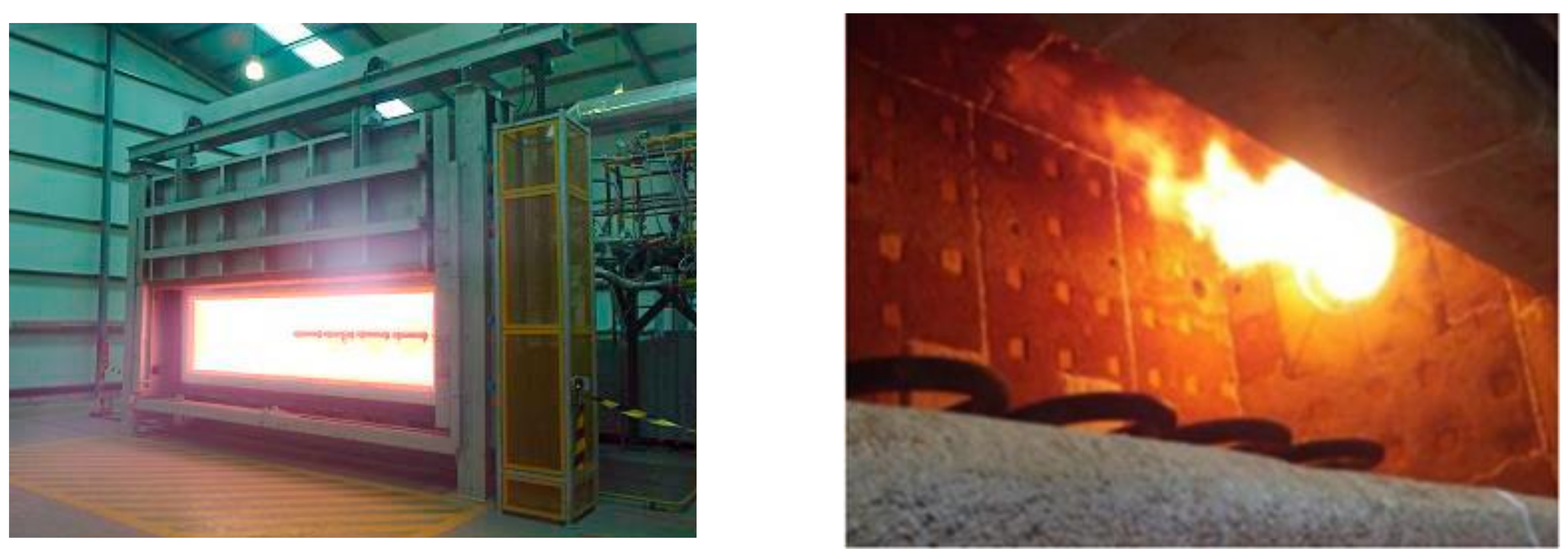
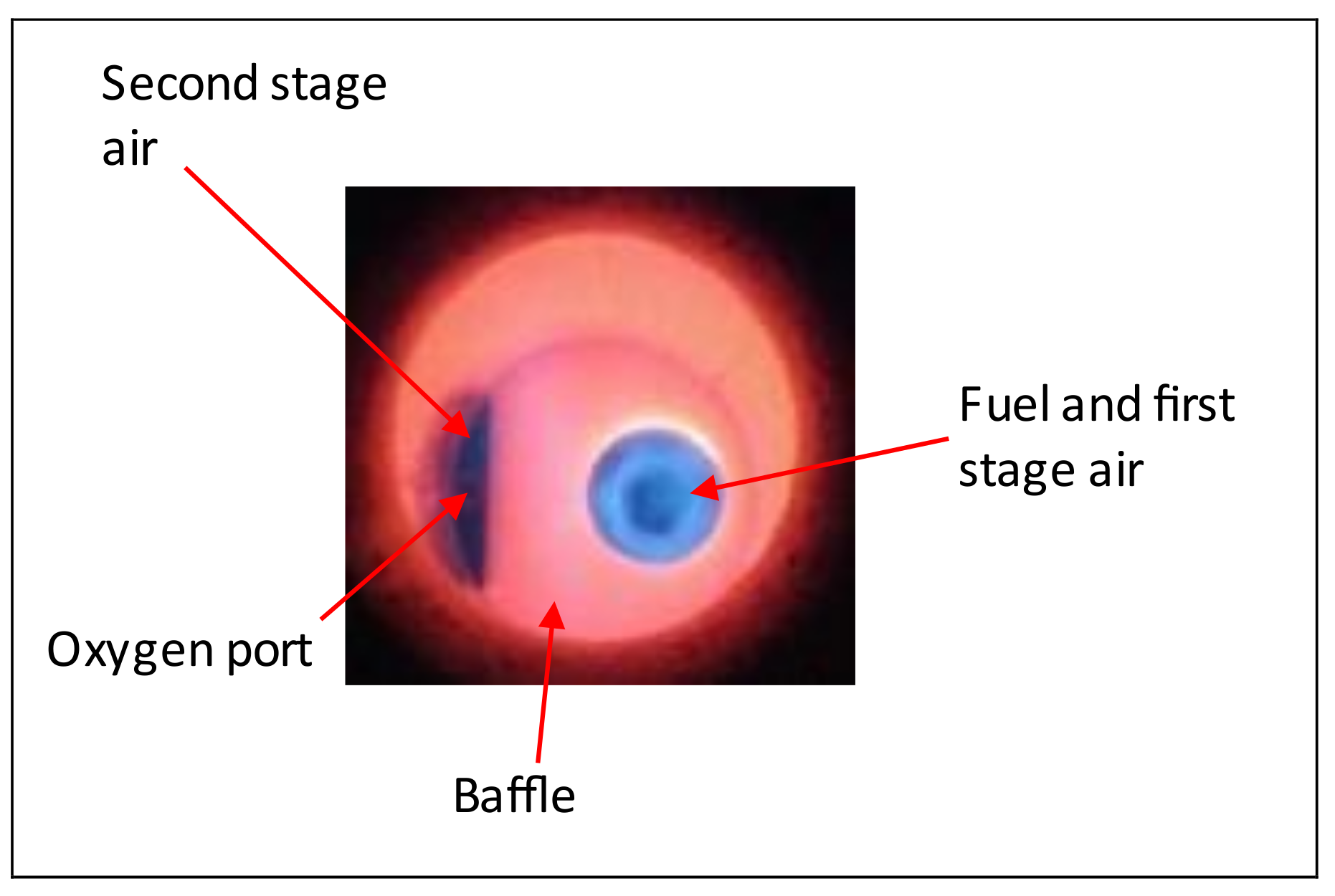
2.1. Test Furnace

The findings presented in this paper are based on an industrial testing furnace located in the ArcelorMittal Asturias (Spain) plant (see Figure 1). This test furnace’s combustion chamber has dimensions of 4.6 m × 1.5 m × 2.8 m and can be equipped with burners with thermal heating capacities of up to 1200 kW, allowing the furnace to reach temperatures of 1400 °C. The fuel-fed system is connected to the off-process gas grid of the plant so it can be fed with real BFGs and coke oven gas (COG) with the same composition and quality as those used in real processes. The furnace is also connected to the NG lines that feed the plant. This has an advantage compared to the use of premixed blends from gas suppliers, as these are of better quality than real gases and can provide more realistic results during the conducted experiments.

During these experimental trials, the furnace was equipped with a low-NOx diffusion burner with a non-symmetrical design, which is commonly used in industrial furnaces in the steel sector.

As shown in Figure 2, the burner is divided into two main parts: a fuel and first-stage air inlet and a secondary air inlet located on the left side of the front of the burner. The fuel and first-stage air ports can be configured to use different ducts for the fed gas depending on the type of fuel (natural gas or off-process gases) that will be burned. In the case of BFG with a low heating value, the volume of fuel that will be introduced needs to be significantly higher than the NG to retain the same thermal power levels; thus, the piping and ports through which the gas is injected need to be adapted. The secondary air inlet also allows the connection of a lance to provide oxygen inside the combustion chamber together with secondary air, which allows the testing of the oxygen-enriched conditions within the furnace.

The thermal load is simulated by six semi-circular lances connected to a water circuit. To simulate the heat transferred from the furnace to a steel strip in an industrial furnace, flowing water circulates in these pipes, receiving part of the energy from the combustion processes. Water enters the circuit through the closest lance to the burner and increases its temperature as the water flows through the rest of the tubes. The water circuit is closed by a fluid cooler that cools the water, which is reintroduced to the lances at low temperatures [22].

The furnace is equipped with a complete control and data acquisition system (DAQ), which allows the registering of physical variables such as flow, temperature, and pressure. In particular, for the temperature inside the furnace, 4 thermocouples are located at different locations within the combustion chamber. The mean of these temperatures is considered the temperature inside the furnace. The test facilities are also equipped with flue gas analyzers capable of measuring the CO, NOx, SO₂, CO₂, and O₂ concentrations. The test furnace can be configured to work with different gaseous blends of the three gaseous fuels available (NG, BFG, and COG) and allows the testing of different configurations, such as the use of preheated combustion air and oxygen injection.

2.2. Experimental Methodology

The methodology used in this study combines CFD simulations with experimental trials used as validations. The furnace was simulated and tested under different fuels and conditions. In particular, for this investigation, the test furnace was fueled with three different fuels, which represent different strategies for improving efficiency and reducing pollutants in steel production processes. These fuels are BFG, NG, and a mixture of 70% BFG/30% NG on a volumetric basis, named BFG, NG, and MIX, respectively, throughout this text. The composition and lower heating values (LHVs) of the fuels are shown in

Table 1. Composition of the gaseous blends used in this study.

	NG	BFG	MIX BFG 70%/NG 30%
CH4	92%	0.01%	27.6%
C2H6	8%	-	2.4%
N2	-	48.98%	34.32%
CO	-	22.34%	15.63%
CO2	-	22.04%	15.42%
H2	-	4.13%	2.89%
H2O	-	1.68%	1.17%
O2	-	0.82%	0.57%
LHV	38,019 kJ/mN3	3270 kJ/mN3	13,690 kJ/mN3

.

The higher the percentage of BFG in the blend, the lower the consumption of NG, which implies savings in fossil fuel consumption and pollutant emissions. However, the blends with a higher share of BFG prevent reaching stable temperatures inside the combustion chamber, which can compromise the quality of the steel produced. Moreover, the lower heating value of BFG requires high gas flows to satisfy the furnace’s demand, which can result in operational problems in bigger furnaces. Thus, the amount of BFG in the blend is limited and the blends require some NG to operate with stability [23].

Table 2. Conditions of the experimental tests.

	NG	BFG	MIX BFG 70%/NG 30%
Furnace temperature	~1347 °C	~1030 °C	~1250 °C
Air excess in fumes	0% vol. O2/ 1.4% vol. O2/ 5.2% vol. O2	0.2% vol. O2/ 1% vol. O2/ 3% vol. O2	0% vol. O2/ 1.1% vol. O2/ 4.4% vol. O2
Air temperature	~500 °C	~500 °C	~500 °C
O2 injection	120 m3N/h	-	-
Fuel thermal power	700 kW	900 kW	700 kW

summarizes the conditions applied for the experimental tests used as validations. The batch of evaluated conditions comprised three different air-to-fuel ratios for each fuel type. The temperature of the furnace, calculated as the mean of the temperature measured at four points in the furnace, was kept constant for each fuel type. Although the power introduced in the furnace with BFG was 200 kW higher than the other fuels, the temperature reached was between 200 °C and 300 °C lower. This is one of the main drawbacks of the use of BFG as the sole fuel; thus, it is often blended with other gaseous fuels with higher heating values.

As shown, for the three fuels, the furnace operated under lean conditions (3–5% of air excess), optimal conditions (1–1.4% of air excess), and rich conditions (0% of air excess). This air-to-fuel ratio was controlled by measuring the oxygen concentration in the fumes while operating. During the trials with NG, an oxygen stream was also introduced as a common strategy for optimizing combustion, which contributed to the temperature increase within the furnace.

The operating strategy differed depending on the type of fuel used. Thus, for NG, the air and fuel flow were kept constant, whereas the oxygen flow was modified in order to obtain the desired air-to-fuel ratio. In the case of BFG as fuel, the fuel flow was also the same for the three cases and the air flow was adjusted to obtain the air-excess conditions. Nevertheless, the use of a mixture of NG and BFG led to the adjustment of both the fuel and air flows to achieve the intended working points, keeping the temperature inside the furnace constant.

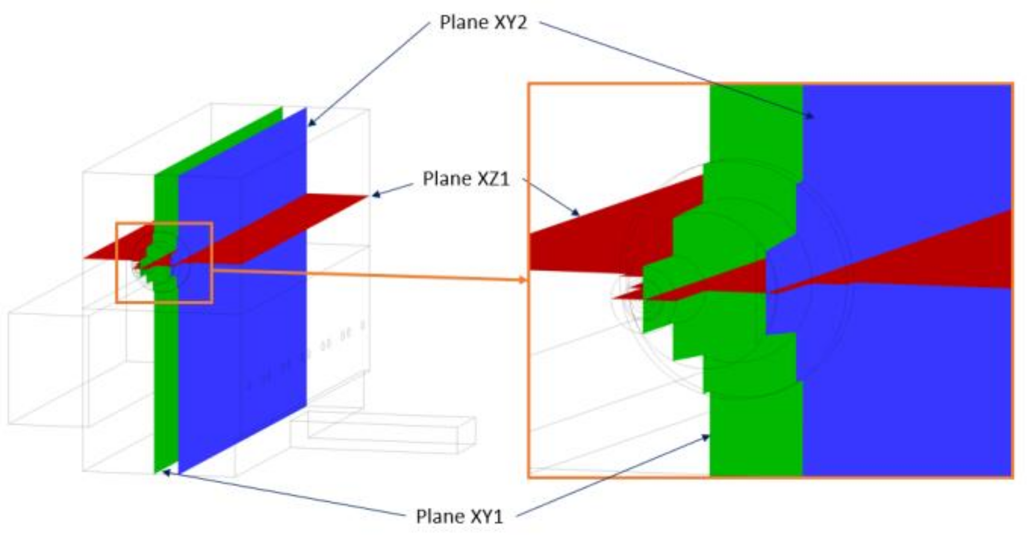
2.3. Furnace Model for CFD Simulation

The furnace geometry was built using the modeling and meshing tools of the Ansys Workbench commercial software. The furnace was divided into subparts in order to apply different mesh strategies depending on the interest of the area. Thus, an adapted mesh with different sizes and types of elements was created. Figure 3 shows a general view of the mesh used.

The burner and lower area of the mesh were built with tetrahedral elements and later converted to a polyhedral using Ansys Fluent 17 functions. Polyhedral elements help reduce stretching and improve the numerical stability of the mesh while reducing the number of elements from 9.4 to 2.5 million cells and, thus, the computational costs [24]. In previous works, the use of polyhedral elements resulted in more accurate results compared to tetrahedral elements, even though the element count was up to 3.4 times lower [25].

Table 3. Mesh quality report.

Mesh Quality Report
Type	Hybrid mesh with polyhedral and hexahedral elements
Number of Elements	2.5 × 106
Minimum Orthogonal Quality	9.54200 × 10−2
Maximum Ortho Skew	0.904580
Maximum Aspect Ratio	24.4659

shows the main characteristics of the mesh.

The sweepable areas with plane faces and straight geometries, such as the upper area, the door, and the outlet zones, were meshed with hexahedral elements, which provided a good combination of accuracy and computational costs.

The air, oxygen, and fuel were introduced into the combustion chamber through ducts with a minimum diameter of 10 mm, which led to elements as small as 2 mm in diameter in order to have good geometry representation in these areas. This ensured good accuracy in these areas, where some of the chemical reactions involved in the combustion process take place. The size slowly increased (1.01 growth rate) as the distance to the burner increased in order to optimize the computational load of the mesh. The thermal load zone elements were also smaller than their surroundings to avoid divergence problems in this area and fully capture the heat transferred to those walls.

The model of the furnace integrated the burner as a boundary condition. For this, only the final zone of the burner was considered, and there was a split in the different gas and air inlets depending on the type of test (fuel mixture, oxidant, etc.) performed.

Fuel gas, oxygen, and secondary air were introduced with a constant mass flow through the corresponding duct in a normal direction to the burner plane. However, the primary air was introduced with a constant mass flow through an axial vane, which generated a swirl of 52°, inducing an axial and tangential component to the velocity. During the experimental tests, the air flow was measured before the burner and distributed inside it between the primary and secondary channels. Based on previous measurements in the facilities, the total air flow was distributed as follows: (1) 27% for primary air, and (2) 73% for secondary air. These were the distribution values used throughout the simulated cases.

The furnace walls were modeled as plain surfaces, where a global heat transfer coefficient was applied. This heat transfer coefficient resulted from the theoretical calculation from a layer model, which considered the forced convection inside the furnace, the conduction of the refractory walls, and the natural convection of the external side of the walls, considering an ambient temperature of 20 °C. A convective boundary condition (Robin condition), where the overall transfer coefficient can be calculated as follows, was chosen:

$$U=\frac{1}{\frac{1}{h_{int}}+\frac{L_1}{k_1}+\frac{L_2}{k_2}+\dots +\frac{L_i}{k_i}+\frac{1}{h_{ext}}}$$

(1)

where $h_{int}$ is the convective heat transfer coefficient inside the furnace, which was obtained during the CFD calculations. $L_i$ and $k_i$ correspond to the width and conductivity of each refractive layer, respectively, and $h_{ext}$ corresponds to the natural convective heat transfer coefficient outside the furnace [26,27].

For the calculation of the heat conductivity via the refractory layers, the walls of the furnace were divided into three groups depending on the composition of the refractory layers: door, floor and sidewalls, and roof. The door was composed of blocks of 300 ceramic fiber blankets. The floor comprised a group of refractory layers: (1) concrete, (2) insulating concrete, and (3) different refractory bricks. Finally, the rest of the walls considered comprised a group of different layers of concrete, insulating concrete, calcium silicate insulation, and mineral fiber. Since the walls contained multiple ports and holes covered with fiber plugs, it was estimated that the refractory layers covered 60% of the surface of the walls for the calculation of the heat transfer coefficients.

The external natural convection term, $h_{ext}$, was calculated by differentiating between the vertical and horizontal walls [26]. For the vertical wall, the coefficient is calculated as follows:

$$h_{ext, v}=\frac{k}{L} {\left(0.825+\frac{0.387R{a}_L{}^{\frac{1}{6}}}{{\left(1+{\left(0.492/Pr\right)}^{\frac{9}{16}}\right)}^{\frac{8}{27}}}\right)}^2, R{a}_L<{10}^{12}$$

(2)

where $k$ is the thermal conductivity of the external layer of the wall, $L$ is the thickness of the layer, $Pr$ is the Prandtl Number taken as a constant, and $R{a}_L$ is the Rayleigh number.

For the calculation of the convection coefficient of the horizontal walls, the following expression is applied:

$$h_{ext, h}=k \frac{0.14 R{a}_L{}^{1/3}}{L}, 2·{10}^7<R{a}_L<3·{10}^{10}$$

(3)

The Rayleigh number is calculated as follows:

$$R{a}_L=\frac{g\beta }{v\alpha }\left(T_s-T_{\infty }\right)L^3$$

(4)

where $g$ is the gravity, $\beta$ is the thermal expansion coefficient of the air, $v$ is the kinematic viscosity, and $\alpha$ is the thermal diffusivity. $T_s$ denotes the temperature of the external wall surface and $T_{\infty }$ denotes the temperature far from the surface, which, as mentioned previously, was estimated at 20 °C.

For the temperature of the outer side of the walls, $T_s$ was estimated thanks to a batch of thermographic images of different parts of the external walls of the furnace. Figure 4 shows some thermographic images of the external walls. As shown, there were some spots in different parts of the wall with different temperatures, °C, and these were located at the different ports and plugs of the furnace. Nevertheless, most areas of the walls remained at lower temperatures, and in order to homogenize the condition of the walls, a value of 100 °C was fixed for these calculations.

As mentioned previously, the thermal load that simulated a real steel strip in an industrial furnace comprised 6 semi-circular lances connected to a water circuit. The water entered the furnace through the closest lance to the burner and dissipated the heat generated during the combustion, increasing its temperature.

One of the main difficulties of simulating the thermal load is that the heat absorption is not constant but oscillates over time. These oscillations were not considered and a mean value was chosen in this model.

The heat transferred through the tube walls was modeled as a convective boundary, where a flow of water received energy from combustion. The mean water temperature under normal working conditions was 40 °C, and the furnace’s temperature was extracted from experimental data reports.

The correlation applied for the convection coefficient was based on a laminar flow (Reynolds number ≈ 135) in circular tubes, where the Nusselt number can be calculated as follows:

$$N{u}_D \equiv \frac{hD}{k}=3.66 T_s=constant$$

(5)

where $h$ is the convection coefficient, $D$ denotes the tube’s diameter, and $k$ is the conductivity of the piping material. For the case where the temperature of the surface was considered constant, $N{u}_D$ had a value of 3.66, which allowed us to obtain the value of $h$ [27].

The next part of the design comprised the election of the models applied relative to the interaction between the turbulence, chemical reactions, and the thermodynamics of the flows that take part in the combustion inside the combustion chamber; these interactions are explained below.

In addition to the complexity of simulating combustion, in the case in this study, there were issues such as the use of low-calorific-value fuels (BFG) and lean conditions, which implied greater instability with respect to the flame. In the cases where the fuel used was natural gas, the use of a second stream of oxidant, together with the air, required additional efforts in the modeling and calculation of the system.

As mentioned previously, BFG, which is an off-process gas of interest in the steel sector, has a very low heating value (around 3000 kJ/Nm³). In order to achieve sufficient combustion temperatures for different steel production processes, mixing BFG with NG is often needed in order to increase the heating value of the mixture. Another strategy commonly used is preheating the combustion air.

The low calorific value of the BFG also implies the need for a piping and burning infrastructure that is sufficient for transferring large volumetric flows of this gas, usually requiring some investment to adapt the current infrastructure.

For the numerical calculations, the conservation of momentum, mass, and energy was solved with a steady-state method based on the Reynolds-averaged Navier–Stokes (RANS) equations in a finite volume. This scheme reduces the computational effort and is widely used for industrial applications [24]. To solve the RANS equations, the commercial CFD code Fluent v17.2 by Ansys was used.

Turbulence was modeled using the standard κ-ω model with two transport equations since it demonstrates better performance for wall-bounded and low-Reynolds-number flows [28]. The model’s constants were kept at the default values and shear flow corrections were activated.

To model the combustion kinetics, two mechanisms were compared during the first stage: the KEE-58, which consists of 17 species and 58 reactions related to C₁ (hydrocarbons with 1 carbon atom), and the DRM-19 mechanism, which is a reduced mechanism derived from the full GRI-Mech 3.0 mechanism and is based on 19 species and 84 reactions [29,30]. The 19 species in the DRM-19 mechanism are H₂, H, O, O₂, OH, H₂O, HO₂, CH₂, CH₂(s), CH₃, CH₄, CO, CO₂, HCO, CH₂O, CH₃O, C₂H₄, C₂H₅, and C₂H₆. They include C₁ and C₂ (hydrocarbons with 1 and 2 carbon atoms) chemistry, which is important not only since NG and the mixture contain ethane but also because some authors state that for methane oxidation, a major pathway for the destruction of methyl radicals is their recombination to an ethane form [31,32].

The fuel used for the comparisons of the mechanisms was BFG operating under baseline conditions with an air excess of 5% and the other variables measured during the experiment. Figure 5 shows a comparison of the temperatures and OH concentrations in the central plane of the burner for the two mechanisms. Despite the differences in the mechanisms, the deviation in the exhaust gases’ temperatures was minimal (20 °C), and both mechanisms predicted almost the same amount of O₂ and CO. Thus, the presence of C₂H₆ in the NG and mixtures, which were not included in the KEE-58 mechanism, together with the acceptable increase in the computational costs, led to the use of the DRM-19 mechanism for these simulations.

For the assessment of the turbulence–chemistry interaction, two different approaches were followed, and both used the non-premixed combustion model. In the case of BFG and the mixtures of NG/BFG, the laminar flamelet model (LFM) was used [33]. The LFM assumes that the turbulent flame comprises an ensemble of small laminar flamelets that evolve by the turbulent mixture flow so that the evolution of the concentration of the species depends only on the mixture fraction and scalar dissipation, which is a parameter that quantifies the deformation of the flame [31,33,34]. The instantaneous species information regarding the mass fraction and temperature in the turbulent flame was calculated by probability density functions (PDFs) (β-function), which are pre-processed and stored in tables [24]. However, this model could not be applied because of the use of a secondary stream (oxygen) in the case of NG as fuel. In this case, the chemical equilibrium approach was followed. Oxygen injection was configured using a two-mixture fraction PDF. The turbulence–chemistry interaction was also calculated using PDF tables when the secondary oxygen injection was present. The integration of the PDG tables with the rest of the boundary conditions is shown in Figure 6.

Regarding heat transfer, the radiative transfer equation of the gaseous mixture was solved with the discrete ordinate technique, and the weighted-sum-of-gray-gases (WSGG) model was used to evaluate the spectral properties of the participating medium [35]. The parameters to configure the angular discretization of the radiation model were theta divisions of 3, phi divisions of 3, theta pixels of 2, and phi pixels of 2. The number of iterations per radiation iteration was reduced from 200 to 20 as the convergence advanced.

On the other hand, the NO_x prediction was decoupled from the main calculation, which implies that the equations of the NO_x model were solved once the solution converged. This is a common procedure because NO_x concentrations influence fluid dynamics and combustion can be neglected. The NO_x thermal model from the commercial CFD code Fluent v17.2 by Ansys was used, including a reburn model [24].

Finally, the criterion followed to ensure the convergence of the solution was based on two aspects. First, the criterion for the residuals was an order of 10⁻⁴, except for NO_x, where a 10⁻⁵ order was selected [36]. Moreover, the stability of the heat transferred to the load, gas outlet temperature, temperature inside the furnace, and oxygen concentration were verified before each case was terminated.

3. Results

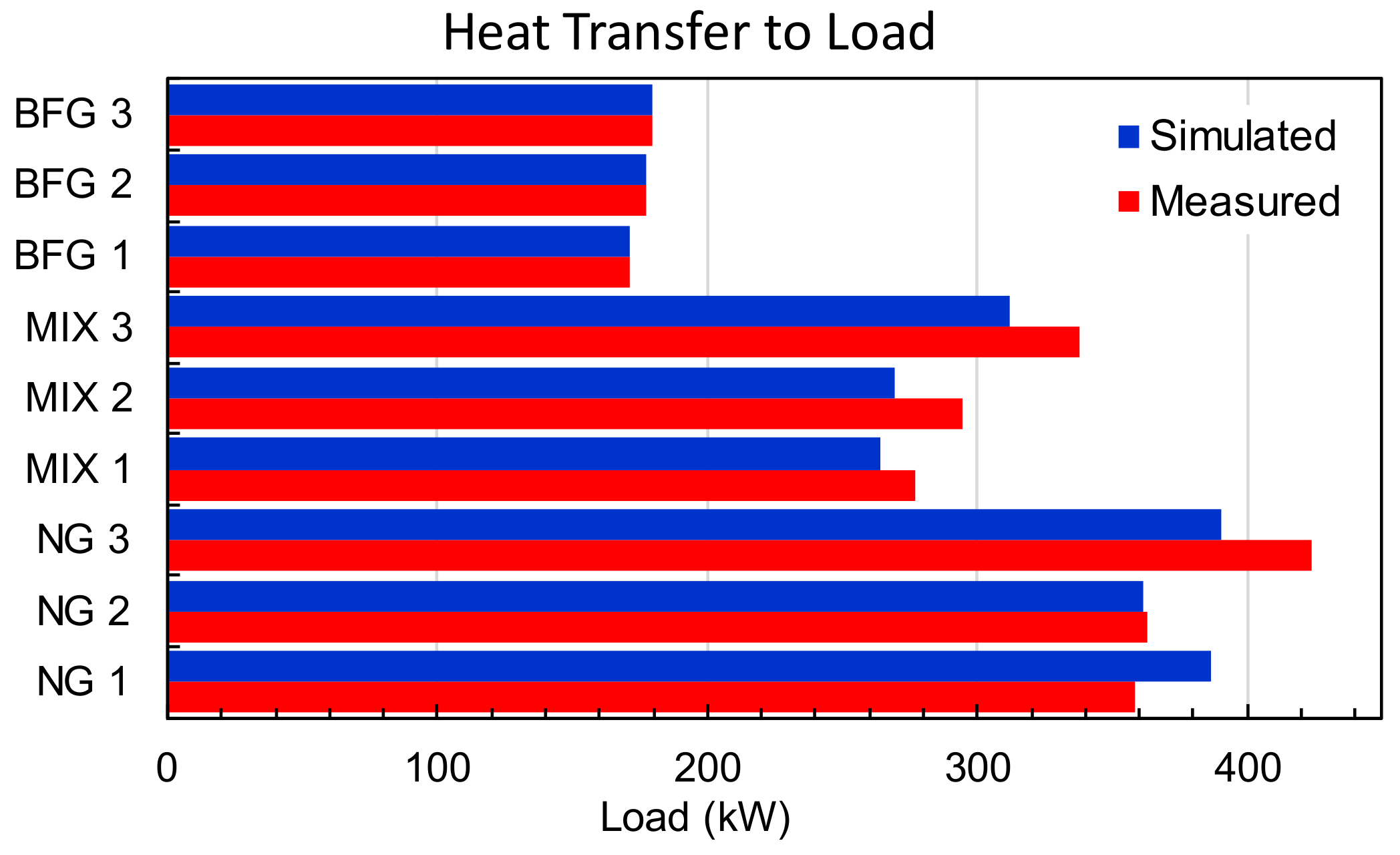
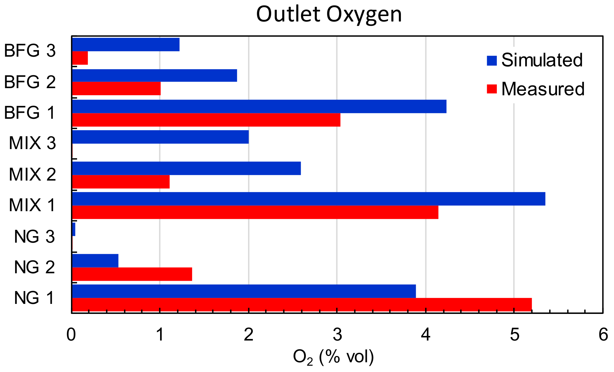
3.1. Model Validation

Before the analysis of the results of the studied cases, model validation was performed by comparing the results obtained from the simulations with the experimental measurements in the industrial furnace. The validation of the simulations with the experimental results proved to be good practice for ensuring the accuracy of the results [37,38].

Table 4. Matrix of tested cases.

	BFG 1	BFG 2	BFG 3	NG 1	NG 2	NG 3	MIX 1	MIX 2	MIX 3
Power (kW)	903.8	900.5	901.6	979.7	735.0	857.4	700.7	698.2	757.8
Fuel temperature (°C)	36.5	34.6	34.6	23.6	22.4	23.0	26.5	24.8	28.4
Air temperature (°C)	528	549	551	449	485	486	495	493	505
Oxygen enrichment	-	-	-	YES	YES	YES	-	-	-
Oxygen excess (%)	3	1	0.2	5.2	1.4	0.0	4.1	1.1	0.0
Fuel–primary air ratio	3.86	4.93	5.38	0.77	0.92	0.98	1.39	1.38	1.52

summarizes the matrix of the scenarios and the inputs used for the CFD cases. As mentioned previously, the test campaign carried out in this study covered different cases with simultaneous changes in the critical combustion parameters, such as the swirl number, fuel/air ratio, power, and type of fuel.

For the obtention of the simulated temperatures and concentrations that can be compared with the experimental measurements, the mean of the elements located in the mesh surface equivalent to the real position of the sensors was obtained.

The first parameter used for validation was the exhaust gas’s temperature. As shown in Figure 7, the outlet temperature increased for the BFG as the equivalence ratio increased since there was less heat wasted when heating the nitrogen that entered the furnace with the primary and secondary air. The difference calculated via CFD for the MIX cases followed the same trend but higher differences in the temperatures were obtained.

The NG cases were quite different as they included enriched oxygen, which was used to modify the equivalence ratio. From the CFD results, it can be deduced that for NG, the combustion was not complete since the outlet CO increased from 0.05 (%v) in NG 1 to 1.9 (%v) in NG 2, whereas for the other fuels, the CO generation was almost negligible. According to the CFD simulations, the amount of lost heat because of bad combustion compensated for the amount of heat reduced from heating the extra oxygen stream; thus, the temperatures were similar for NG 1 and NG 2. In contrast, the NG 3 case experienced more energy introduced with the fuel and had the same equivalence ratio as NG 2. In this case, although the CFD captured higher temperatures, the temperature measured during the test was lower than in previous cases.

However, the heat transferred to the load (see Figure 8) was directly related to the furnace’s temperature and the total flow introduced to the furnace. For BFG and NG, it was well captured, whereas for MIX, it was underpredicted. This seems reasonable considering the previous analysis regarding the outlet temperature. The differences in the temperature and heat transfer could also be related to the fluctuating values of the temperature and, consequently, to the load used during the test.

Finally, Figure 9 shows a comparison of the measurements of the oxygen concentration in the outlet port and the results of the simulations. As shown, for the cases of BFG and MIX, the CFD overestimated the oxygen concentration, whereas for the NG case, there was an opposite trend. Several factors influenced the final measured concentration, which in the case of the simulation, was computed from the flow’s boundary conditions. Among these factors, several windows and ports exist, which caused infiltrations or leakages of air depending on the combustion chamber’s pressure, and this contributed to the modification of the theoretical balances and differed from the boundary conditions used for the simulations.

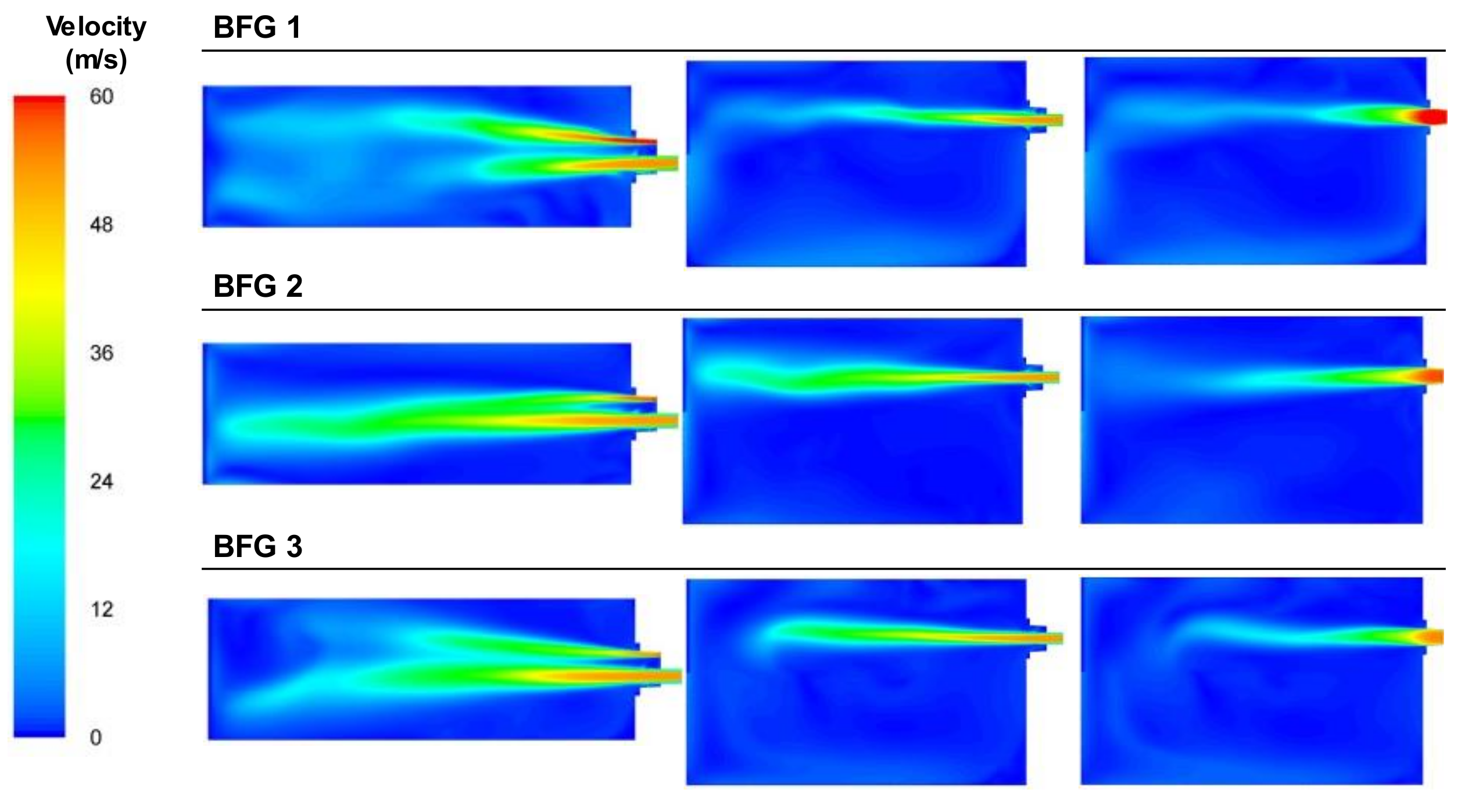
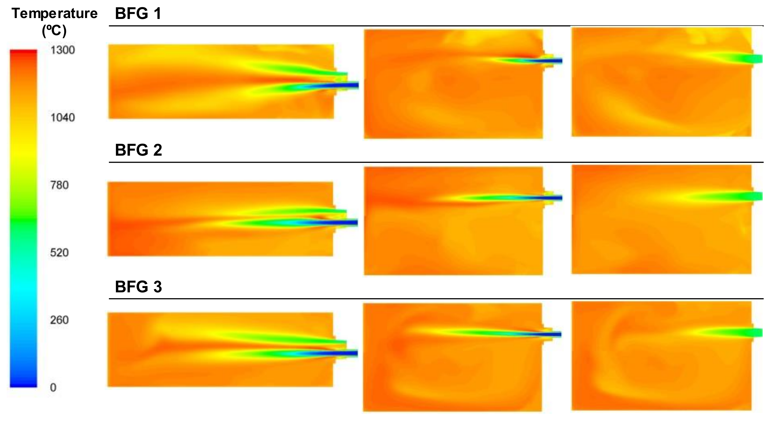
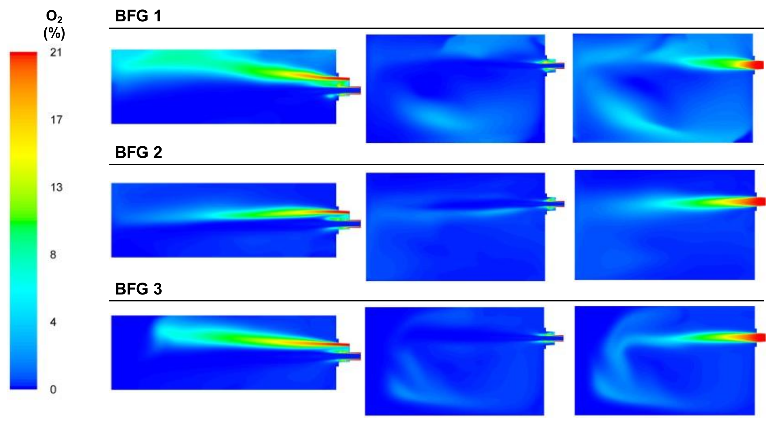
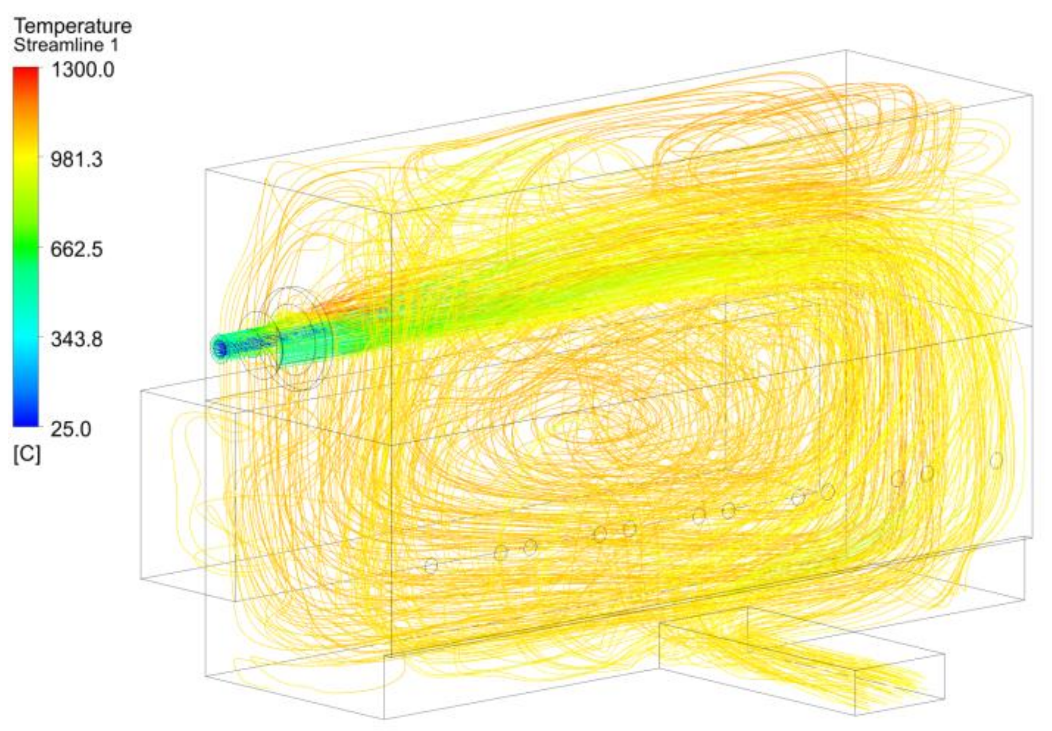
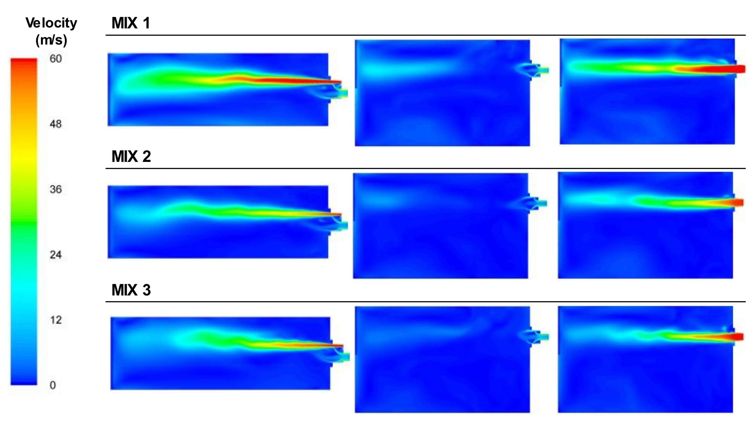
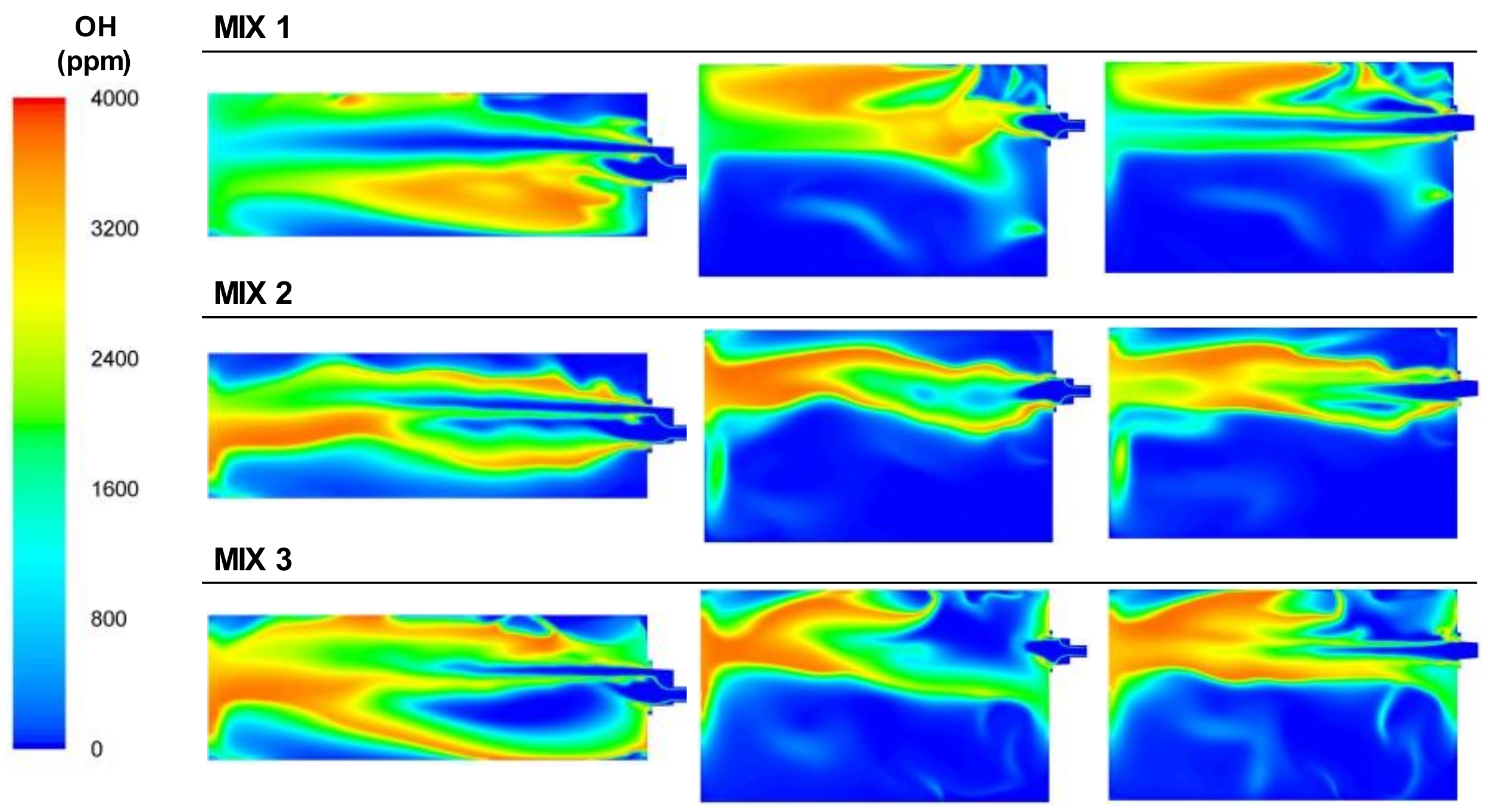
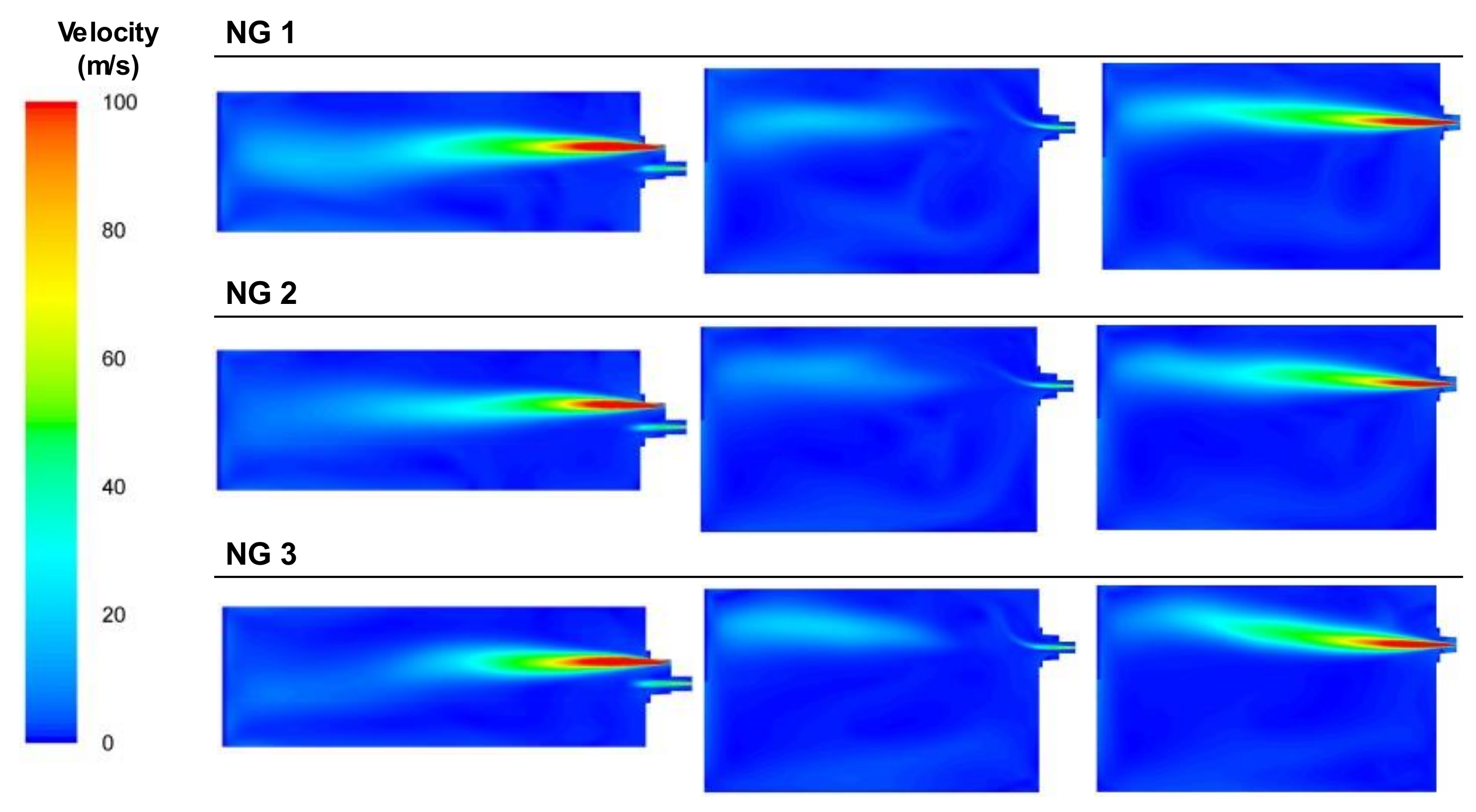
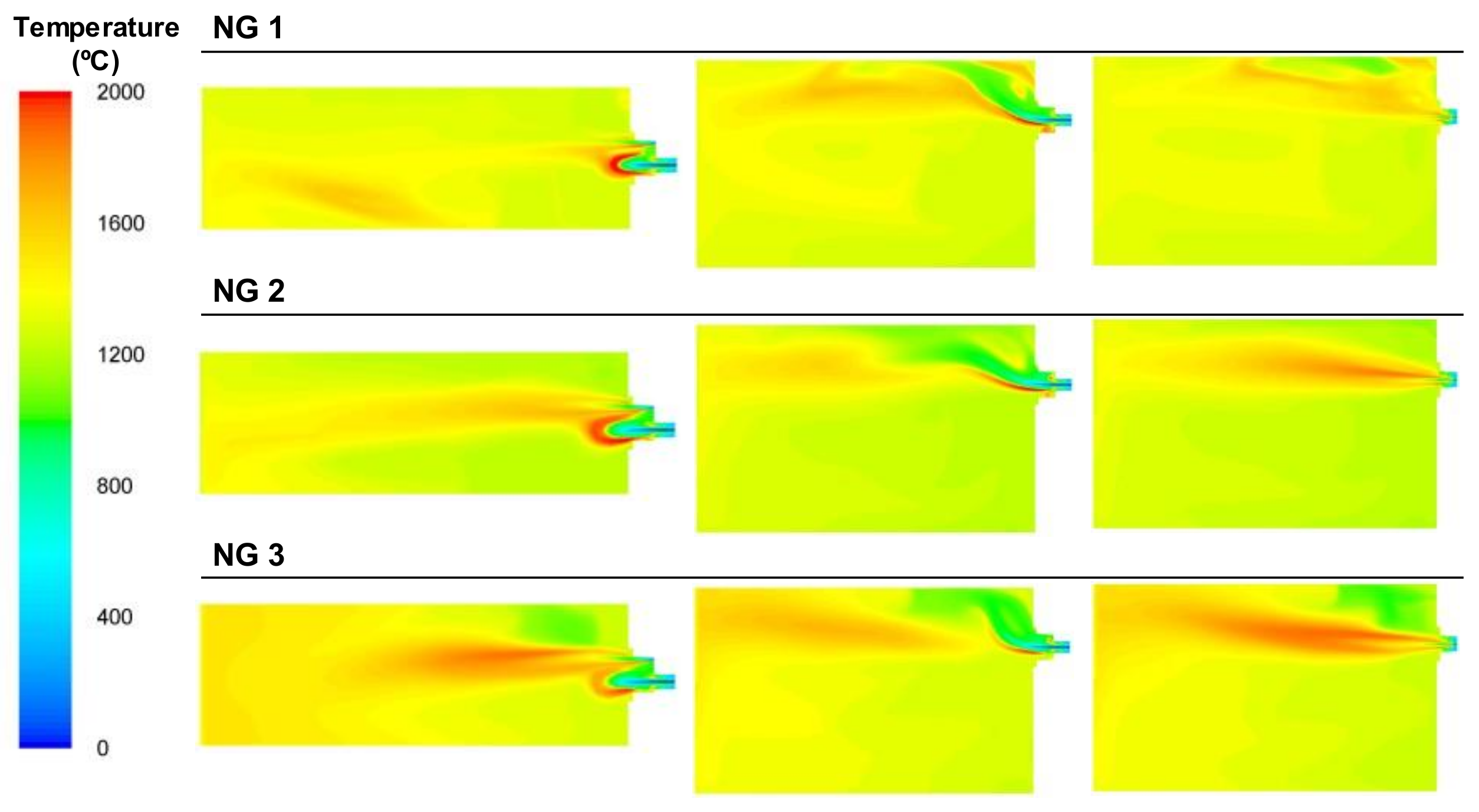
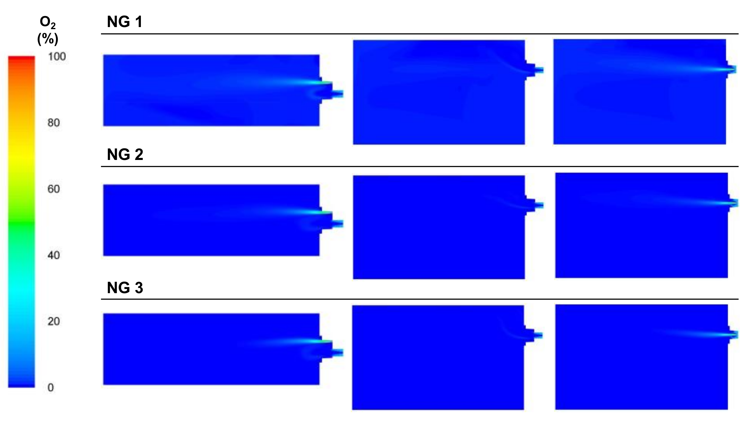
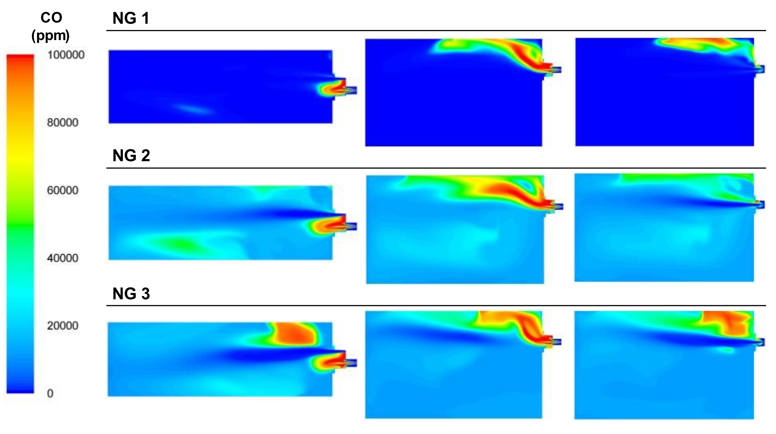
3.2. Results Analysis and Discussion

This section explains the results of the calculations of the furnace with the three gaseous fuels working under the conditions described previously. The representative surfaces chosen to present the different plots of the most relevant physical variables are presented in Figure 10. Plane XZ1 corresponds to the horizontal plane passing through the center of the burner, Plane XY1 corresponds to the vertical plane through the center of the burner, and Plane XY2 corresponds to the vertical plane passing through the center of the secondary air and oxygen inlets.

For BFG, the use of a low-calorific-value gas prevented the furnace from reaching its set point temperature (usually 1300 °C) since to reach typical operating set points, it would be necessary to preheat a gas or use oxygen-enhanced combustion [22]. However, these conditions were chosen considering this fact and aimed to explore the limits of the installation and the models developed. Moreover, the use of 100% BFG in the combustion processes is of great interest in the steel industry in order to increase the efficiency of the entire process [11].

Figure 11 presents the plot of the velocity for the three cases that used BFG as the fuel. The velocities in areas closest to the fuel and air inlets remained constant in the area where BFG was the main component and decreased as the flow of air was reduced, especially in the secondary air inlet area. BFG 1, which was the leaner case, showed a shorter flame, whereas in the other cases, the combustion zones increased, as the fuel and air streams needed more space to mix and burn.

Figure 12 shows the temperature plots that, in general, looked similar for the three cases throughout the furnace because of the small differences in the power inputs of those cases. The area with the maximum temperature was located between the fuel/primary air stream and the secondary air stream, which was introduced and preheated at temperatures over 500 °C. Combustion started with the primary air and continued when it reached the heated oxygen introduced via the secondary air duct. Both Figure 11 and Figure 12 show long flames, where the swirl effect induced by the primary air’s rotation was not enough to break the inertia of the high fuel flow. Thus, the flame extended and shifted closer to laminar combustion patterns.

In the burner area where the combustion took place, the way the combustion flame extended as the air flow decreased can be deduced from the temperature plots. This is confirmed by the plots of the OH concentrations, which were often related to the flame’s front development. Figure 13 includes the plots of the OH concentration for the BFG cases, where it can be seen how the OH production occurred far from the inlets as the air flow decreased. It can also be seen how the fluid dynamics inside the furnace, with large flow streams and recirculated streams, caused the highest OH concentrations to deviate from the flame front, as expected.

Regarding the oxygen concentration, Figure 14, which includes the plots of the oxygen concentration from the analysis sections, shows that the oxygen that left the burner area without participating in the combustion processes decreased in the cases with lower air flows. This was reflected in the final concentration of oxygen in the exhaust gas area.

As shown in Figure 15, the NOx generation in the case of BFG was low since the temperature of the combustion was the lowest out of all the fuels, even though in the cases with air excess, there was oxygen available for nitrogen oxidation. The combustion temperatures were similar for the three air-to-fuel ratio cases so all cases presented nearly the same generation of NOx. The areas with NOx rate generation can be observed. Thermal NOx production happened in areas with high temperatures and enough oxygen concentration, and this can be observed in the contours of the NOx rate, oxygen, and temperature.

The final analysis of the BFG was the streamlining of the temperatures, which allowed a global view of the fluid dynamics inside the combustion chamber (see Figure 16). The high flows needed to maintain the power inside the combustion chamber produced a high stream of burned gas, which collided with the wall opposite the burner and recirculated through the furnace. An important part of the gases recirculated below the load area to the burner wall, where it proceeded to the top of the furnace. This also explains how the convection heat transferred in the water lances closest to the burner was greater in the bottom part of the lances, whereas the main transfer was produced through the upper section of the water lances further away from the burner.

The next analysis covered the results of the furnace for the MIX cases, which corresponded to a mixture of 70% vol. BFG and 30% vol. NG, 89% NG, and 11% BFG on an LHV basis. The three cases tested covered the three different air-to-fuel ratios from lean conditions to sub-stoichiometric conditions, but unlike the BFG cases where the air excess was controlled with the air flow, they were modified both with respect to the fuel and air flows in order to operate under the desired conditions. The furnace worked under different load conditions; thus, the results were more heterogeneous than in the case of the BFG as the sole fuel.

Figure 17 presents the velocity plots for the three mixture cases tested. As can be observed, the velocity of the fuel mixture was low compared to the air velocity. The addition of natural gas to the BFG increased the heating value of the mixture; thus, the mass flow of the fuel decreased significantly compared with the BFG cases. In this case, the effect of the swirl of the primary air appeared, in contrast to the case of BFG. The swirl affected the combustion by opening and shortening the flame. Thus, it no longer developed with a classical flame structure.

The effect of the NG in the mixture was also noted in the temperatures reached, which were significantly higher than those in the BFG case, as can be observed in the Figure 18. In the cases where the fuel used was BFG, the area with the highest temperatures was located in the zone where the fuel and primary air interacted with the secondary air stream. There were two main zones of combustion: one in the area of the fuel outlet using the primary air and the oxygen in the surroundings and another around the secondary air jet.

The OH concentrations, presented in Figure 19, performed in a similar way to the BFG, where the contours of the concentrations of OH were mostly influenced by the internal recirculation of the gases inside the furnace rather than its own flame shape due to the recirculating flows inside the furnace.

It can also be seen in Figure 20 that the concentration of oxygen decreased throughout the furnace for the MIX 2 and MIX 3 cases compared to MIX 1 since the excess air decreased and most of the oxygen participated in the combustion.

Regarding the NOx, Figure 21 shows the areas where the NOx was generated. Since the temperatures reached were higher than those in the BFG cases, the NOx emissions with this fuel exceeded those using BFG. The main areas of NOx generation were located in the high-temperature zones between the primary and secondary streams, where there was oxygen available.

The analysis of the streamlines for the mixture case presented in Figure 22, shows that even though the behaviors of the fuel and air flows were quite different from the BFG case, the recirculation of the combustion gases favored the convection water lances that were more distant from the burner.

The final analysis was carried out for the natural gas enriched with a stream of oxygen. Oxy-combustion improved the efficiency since a part of the liberated energy during the combustion when the air was used as an oxidant was transferred to heat the percentage of nitrogen. In the case of oxy-combustion, the absence of nitrogen allowed this energy to be transferred to the load. As explained previously, the cases of natural gas required a different model for the simulation since there was an additional oxidant stream, which was the pure oxygen injected through the lance installed in the secondary air inlet.

For these cases, the regulation of the air-to-fuel ratio was achieved by modifying the rate of pure oxygen injected and the fuel, whereas the air flows were kept almost constant.

Figure 23 presents the plots of the velocities for the three NG cases. As shown, the injection of a high amount of oxygen through a lance with a small diameter (see Figure 24) led to high velocities in the combustion mixture. The natural gas was also introduced into the smallest diameter orifice of the burner but its velocity was lower compared to the oxygen.

The use of NG, which has the highest calorific value of all the fuels tested, together with the use of pure oxygen, decreased the amount of inert gases, as there was nitrogen from the BFG and air or CO₂ contained in the fuel, and the temperature inside the furnace was the highest out of all the cases, as illustrated in Figure 24. In these cases, combustion started in the area next to the burner’s head but was strongly affected by the flow of oxygen, as shown in Figure 25. The OH concentration in the case of NG 1 was focused through the top of the burner, whereas in NG 2 and NG 3, this phenomenon was less significant. The stream of pure oxygen, which flowed at the highest velocity, displaced the fuel and air streams and contributed to increasing the concentration of oxygen in the entire furnace instead of reacting with the NG in the burner zone. Unlike the BFG and mixture cases, for NG, the contours of the maximum OH concentrations corresponded to the flame front.

The oxygen concentrations of the cases are shown in Figure 26. The oxygen calculated at the outlet port followed the experimental trend since the air flow was maintained and the oxygen flow decreased from NG 1 to NG 3. The absence of oxygen led to incomplete combustion in the NG 2 and NG 3 cases; thus, the CO concentrations increased (see Figure 27).

The NOx rates of the NG cases are shown in Figure 28. The high combustion temperatures and the presence of oxygen in the area immediately after the burner favored the NOx generation in this zone. At high combustion temperatures, the thermal production of NOx doubled for every 90 °C of temperature [24]. Another factor that contributed to this generation was the turbulence caused by the swirl of the primary air, which in the BFG case, was masked by the high flow rates of the fuels.

Finally, Figure 29 presents the streamlines of the temperature for the NG1 case. In this case, the flow of primary fuel and air conformed to a short flame, whereas the high velocities of the oxygen stream influenced the distribution of the gases inside the furnace.

4. Conclusions

This paper presents the validation and results of a CFD model of an industrial test furnace in the steel sector used to analyze solutions (burners, conditions, and fuel mixtures) before their application to real processes. The model allows for the study of the combustion of different gaseous mixtures (NG, BFG, and mixtures) and considers all the relevant phenomena within the furnace: radiation, pure oxygen stream, heat transfer through the walls, load, turbulence, pollutant formation, and combustion. In general, the theoretical results obtained agree well with the results from the experiments carried out during the tests performed under the same conditions. The most relevant conclusions obtained from this study are as follows:

• The use of very different heating value fuels leads to different fluid dynamics since very different volumetric flows are introduced to produce similar powers. Burning equipment must be adapted to ensure flame geometries, and this will imply different nozzles and swirling methods.
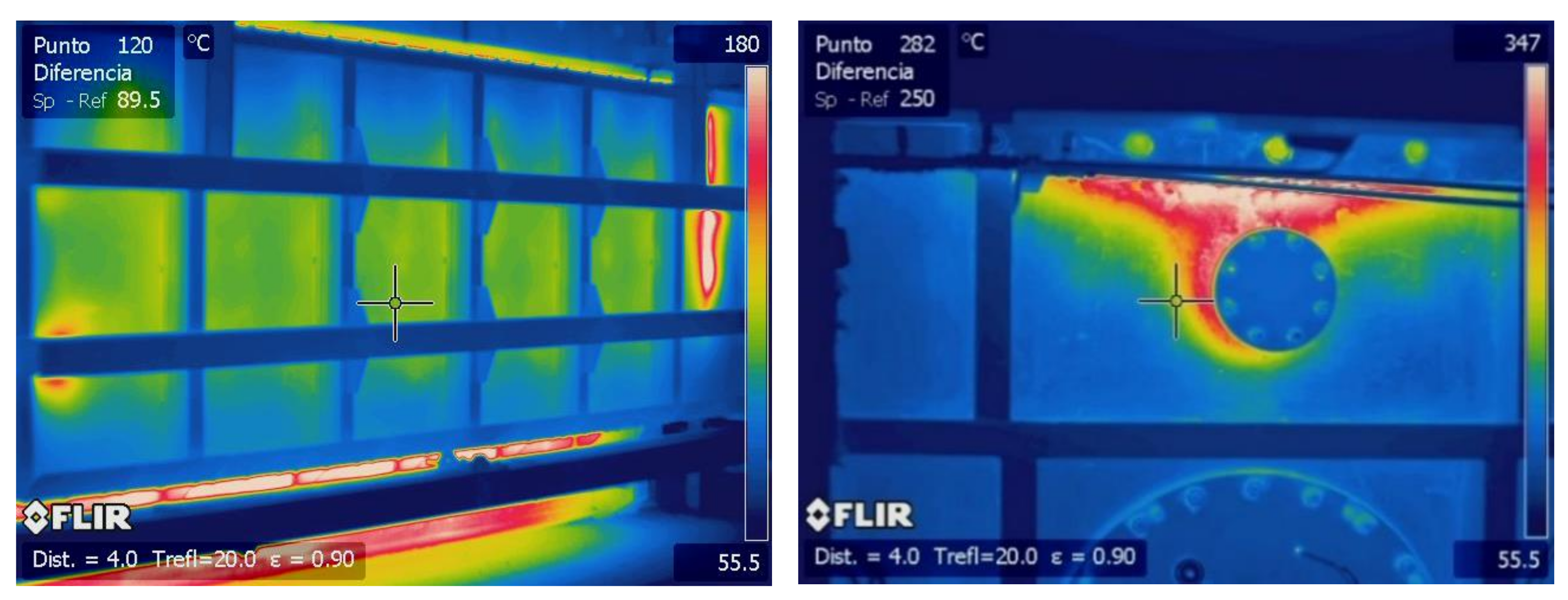
• Thus, the heat transferred to the load is not homogeneous. The flow pattern inside the furnace causes differences in the heat transfer distribution along the load walls. Usually, the heat transfer to the real load in the steel sector is critical so the use of different calorific value gases can affect the quality of the process (different temperature gradients in the load).
• The swirl effect and the flame geometry are highly dependent on the flow ratio between the primary and secondary air, and between the primary air and fuel. Although the swirl effect is neglected in the BFG cases, the MIX cases rotate and produce short flames.
• The flow of BFG needs to be doubled in order to obtain similar temperatures to those reached by NG combustion. These high flow rates may exceed the installation limits, thus requiring additional investment. Oxy-combustion is an option for overcoming this problem.

References

1. Nandhini, R.; Sivaprakash, B.; Rajamohan, N. Waste Heat Recovery at Low Temperature from Heat Pumps, Power Cycles and Integrated Systems–Review on System Performance and Environmental Perspectives. Sustain. Energy Technol. Assess. 2022, 52, 102214. [Google Scholar] [CrossRef]
2. Wang, X.; Li, C.; Lam, C.H.; Subramanian, K.; Qin, Z.-H.; Mou, J.-H.; Jin, M.; Chopra, S.S.; Singh, V.; Ok, Y.S.; et al. Emerging Waste Valorisation Techniques to Moderate the Hazardous Impacts, and Their Path towards Sustainability. J. Hazard Mater. 2022, 423, 127023. [Google Scholar] [CrossRef] [PubMed]
3. Pierri, E.; Hellkamp, D.; Thiede, S.; Herrmann, C. Enhancing Energy Flexibility through the Integration of Variable Renewable Energy in the Process Industry. Procedia CIRP 2021, 98, 7–12. [Google Scholar] [CrossRef]
4. Sun, Y.; Tian, S.; Ciais, P.; Zeng, Z.; Meng, J.; Zhang, Z. Decarbonising the Iron and Steel Sector for a 2 °C Target Using Inherent Waste Streams. Nat. Commun. 2022, 13, 297. [Google Scholar] [CrossRef]
5. Huth, M.; Heilos, A. 14-Fuel Flexibility in Gas Turbine Systems: Impact on Burner Design and Performance. In Modern Gas Turbine Systems; Jansohn, P., Ed.; Woodhead Publishing Series in Energy; Woodhead Publishing: Sawston, UK, 2013; pp. 635–684. ISBN 978-1-84569-728-0. [Google Scholar]
6. Chen, H.; Wang, Y.; Yan, L.; Wang, Z.; He, B.; Fang, B. Energy and Exergy Analysis on a Blast Furnace Gas-Driven Cascade Power Cycle. Energies 2022, 15, 8078. [Google Scholar] [CrossRef]
7. Smil, V. Chapter 7-Energy Costs and Environmental Impacts of Iron and Steel Production: Fuels, Electricity, Atmospheric Emissions, and Waste Streams. In Still the Iron Age; Smil, V., Ed.; Butterworth-Heinemann: Boston, MA, USA, 2016; pp. 139–161. ISBN 978-0-12-804233-5. [Google Scholar]
8. Bailera, M.; Nakagaki, T.; Kataoka, R. Limits on the Integration of Power to Gas with Blast Furnace Ironmaking. J. Clean Prod. 2022, 374, 134038. [Google Scholar] [CrossRef]
9. Xu, Y.-P.; Liu, R.-H.; Shen, M.-Z.; Lv, Z.-A.; Chupradit, S.; Metwally, A.S.M.; Sillanpaa, M.; Qian, Q. Assessment of Methanol and Electricity Co-Production Plants Based on Coke Oven Gas and Blast Furnace Gas Utilization. Sustain. Prod. Consum. 2022, 32, 318–329. [Google Scholar] [CrossRef]
10. Khallaghi, N.; Abbas, S.Z.; Manzolini, G.; de Coninck, E.; Spallina, V. Techno-Economic Assessment of Blast Furnace Gas Pre-Combustion Decarbonisation Integrated with the Power Generation. Energy Convers. Manag. 2022, 255, 115252. [Google Scholar] [CrossRef]
11. Cuervo-Piñera, V.; Cifrián-Riesgo, D.; Nguyen, P.D.; Battaglia, V.; Fantuzzi, M.; della Rocca, A.; Ageno, M.; Rensgard, A.; Wang, C.; Niska, J.; et al. Blast Furnace Gas Based Combustion Systems in Steel Reheating Furnaces. In Proceedings of the Energy Procedia; Elsevier Ltd.: Amsterdam, The Netherlands, 2017; Volume 120, pp. 357–364. [Google Scholar]
12. Musiał, D. Coke and Blast Furnace Gases: Ecological and Economic Benefits of Use in Heating Furnaces. Combust. Sci. Technol. 2020, 192, 1015–1027. [Google Scholar] [CrossRef]
13. Zhang, L.; Xie, W.; Ren, Z. Combustion Stability Analysis for Non-Standard Low-Calorific Gases: Blast Furnace Gas and Coke Oven Gas. Fuel 2020, 278, 118216. [Google Scholar] [CrossRef]
14. Paubel, X.; Cessou, A.; Honore, D.; Vervisch, L.; Tsiava, R. A Flame Stability Diagram for Piloted Non-Premixed Oxycombustion of Low Calorific Residual Gases. Proc. Combust. Inst. 2007, 31, 3385–3392. [Google Scholar] [CrossRef]
15. Caillat, S. Burners in the Steel Industry: Utilization of by-Product Combustion Gases in Reheating Furnaces and Annealing Lines. In Proceedings of the Energy Procedia; Elsevier Ltd.: Amsterdam, The Netherlands, 2017; Volume 120, pp. 20–27. [Google Scholar]
16. Bâ, A.; Cessou, A.; Marcano, N.; Panier, F.; Tsiava, R.; Cassarino, G.; Ferrand, L.; Honoré, D. Oxyfuel Combustion and Reactants Preheating to Enhance Turbulent Flame Stabilization of Low Calorific Blast Furnace Gas. Fuel 2019, 242, 211–221. [Google Scholar] [CrossRef]
17. Compais, P.; Arroyo, J.; González-Espinosa, A.; Castán-Lascorz, M.Á.; Gil, A. Optical Analysis of Blast Furnace Gas Combustion in a Laboratory Premixed Burner. ACS Omega 2022, 7, 24498–24510. [Google Scholar] [CrossRef]
18. Chattopadhyay, K.; Isac, M.; Guthrie, R.I.L. Applications of Computational Fluid Dynamics (CFD) in Iron- and Steelmaking: Part 1. Ironmak. Steelmak. 2010, 37, 554–561. [Google Scholar] [CrossRef]
19. Chattopadhyay, K.; Isac, M.; Guthrie, R.I.L. Applications of Computational Fluid Dynamics (CFD) in Iron- and Steelmaking: Part 2. Ironmak. Steelmak. 2010, 37, 562–569. [Google Scholar] [CrossRef]
20. Ma, X.; Zhang, S.; Yu, H.; Qi, G. Numerical Simulation of Combustion and Emission of Blast Furnace Gas Boiler. IOP Conf. Ser. Mater Sci. Eng. 2020, 721, 012042. [Google Scholar] [CrossRef]
21. Liu, Y.Q.; Wang, X.Y.; Zhu, G.F.; Liu, R.X.; Gao, Z.Q. Simulation on the Combustion Property of Blast-Furnace Gas Engine by GT-POWER. In Proceedings of the Advanced Manufacturing Technology, ICAMMP 2010, Guilin, China, 16–18 December 2011; Trans Tech Publications Ltd.: Bäch, Switzerland, 2011; Volume 156, pp. 965–968. [Google Scholar]
22. Directorate-General for Research and Innovation (European Commission); Battaglia, V.; Niska, J.; Cuervo Piñera, V.; Fantuzzi, M.; Wang, C.; Rensgard, A.; Cifrián Riesgo, D. High Efficiency Low NOX BFG Based Combustion Systems in Steel Reheating Furnaces (HELNOx-BFG): Final Report; Publications Office: Brussels, Belgium, 2018. [Google Scholar]
23. Zheng, W.; Pang, L.; Liu, Y.; Xie, F.; Zeng, W. Effects of Methane Addition on Laminar Flame Characteristics of Premixed Blast Furnace Gas/Air Mixtures. Fuel 2021, 302, 121100. [Google Scholar] [CrossRef]
24. ANSYS, Inc. Fluent User’s Guide, Release 17.2; ANSYS, Inc.: Canonsburg, PA, USA, 2016. [Google Scholar]
25. Sosnowski, M.; Krzywanski, J. Gnatowska Renata Polyhedral Meshing as an Innovative Approach to Computational Domain Discretization of a Cyclone in a Fluidized Bed CLC Unit. E3S Web Conf. 2017, 14, 1027. [Google Scholar] [CrossRef] [Green Version]
26. Incropera, F.P. Fundamentals of Heat and Mass Transfer; John Wiley & Sons, Inc.: Hoboken, NJ, USA, 2006; ISBN 0470088400. [Google Scholar]
27. Belmiloudi, A. Heat Transfer; IntechOpen: Rijeka, Croatia, 2011. [Google Scholar]
28. Wilcox, D.C. Turbulence Modeling for CFD, 2nd ed.; DCW Indstries: La Cañada, CA, USA, 2006. [Google Scholar]
29. Chang, W.-C.; Chen, J.-Y. Available online: http://firebrand.me.berkeley.edu/griredu.html (accessed on 1 October 2019).
30. Smith, G.P.; Golden, D.M.; Frenklach, M.; Moriarty, N.W.; Eiteneer, B.; Goldenberg, M.; Bowman, C.T.; Hanson, R.K.; Song, S.; Gardiner, W.C., Jr.; et al. Available online: http://combustion.berkeley.edu/gri-mech/version30/text30.html (accessed on 1 October 2019).
31. de Joannon, M.; Saponaro, A.; Cavaliere, A. Zero-Dimensional Analysis of Diluted Oxidation of Methane in Rich Conditions. Proc. Combust. Inst. 2000, 28, 1639–1646. [Google Scholar] [CrossRef]
32. Aminian, J.; Galletti, C.; Shahhosseini, S.; Tognotti, L. Numerical Investigation of a MILD Combustion Burner: Analysis of Mixing Field, Chemical Kinetics and Turbulence-Chemistry Interaction. Flow Turbul. Combust. 2012, 88, 597–623. [Google Scholar] [CrossRef]
33. Peters, N. Laminar Flamelet Concepts in Turbulent Combustion; Elsevier: Amsterdam, The Netherlands, 1988. [Google Scholar]
34. Benim, A.C.; Syed, K.J. Laminar Flamelet Modelling of Turbulent Premixed Combustion. Appl. Math. Model. 1998, 22, 113–136. [Google Scholar] [CrossRef]
35. Hottel, H.C.; Saroffim, A.F. Radiative Heat Transfer; McGraw-Hill: New York, NY, USA, 1967. [Google Scholar]
36. Khoshhal, A.; Rahimi, M.; Alsairafi, A.A. CFD Study on Influence of Fuel Temperature on NOx Emission in a HiTAC Furnace. Int. Commun. Heat Mass Transf. 2011, 38, 1421–1427. [Google Scholar] [CrossRef]
37. Tominaga, Y.; Shirzadi, M. RANS CFD Modeling of the Flow around a Thin Windbreak Fence with Various Porosities: Validation Using Wind Tunnel Measurements. J. Wind. Eng. Ind. Aerodyn. 2022, 230, 105176. [Google Scholar] [CrossRef]
38. Jayarathna, C.K.; Balfe, M.; Moldestad, B.E.; Tokheim, L.-A. Comparison of Experimental Results from Operating a Novel Fluidized Bed Classifier with CFD Simulations Applying Different Drag Models and Model Validation. Processes 2022, 10, 1855. [Google Scholar] [CrossRef]
Figure 1. ArcelorMittal experimental industrial furnaces located in the Asturias (Spain) plant [22].
Processes 11 00332 g001
Figure 2. Image of the Bloom 1610 burner used for this study.
Processes 11 00332 g002
Figure 3. General view and parts of the mesh of the test furnace.
Processes 11 00332 g003
Figure 4. Samples of thermographic images used for boundary definitions.
Processes 11 00332 g004
Figure 5. Comparison of the (a) temperatures and (b) OH mass fractions of the burner’s central plane for the KEE-58 and DRM-19 mechanisms with BFG as fuel and an air excess of 4%.
Processes 11 00332 g005
Figure 6. Schematic of the boundary conditions used.
Processes 11 00332 g006
Figure 7. Comparison of exhaust temperatures measured and simulated.
Processes 11 00332 g007
Figure 8. Comparison of transferred heat to the load measured and simulated.
Processes 11 00332 g008
Figure 9. Comparison of oxygen concentrations measured and simulated.
Processes 11 00332 g009
Figure 10. Surfaces used for postprocessing.
Processes 11 00332 g010
Figure 11. Contour plots of velocities for the BFG cases in the XZ1, XY1, and XY2 planes.
Processes 11 00332 g011
Figure 12. Contour plots of temperatures for the BFG cases in the XZ1, XY1, and XY2 planes.
Processes 11 00332 g012
Figure 13. Contour plots of OH concentrations for the BFG cases in the XZ1, XY1, and XY2 planes.
Processes 11 00332 g013
Figure 14. Contour plots of oxygen concentrations for the BFG cases in the XZ1, XY1, and XY2 planes.
Processes 11 00332 g014
Figure 15. Contour plots of thermal NOx rate generation for the BFG cases in the XZ1, XY1, and XY2 planes.
Processes 11 00332 g015
Figure 16. Temperature streamlines for the BFG 1 case.
Processes 11 00332 g016
Figure 17. Contour plots of velocities for the BFG/NG mixture cases in the XZ1, XY1, and XY2 planes.
Processes 11 00332 g017
Figure 18. Contour plots of temperatures for the BFG/NG mixture cases in the XZ1, XY1, and XY2 planes.
Processes 11 00332 g018
Figure 19. Contour plots of OH concentrations for the BFG/NG mixture cases in the XZ1, XY1, and XY2 planes.
Processes 11 00332 g019
Figure 20. Contour plots of oxygen concentrations for the BFG/NG mixture cases in the XZ1, XY1, and XY2 planes.
Processes 11 00332 g020
Figure 21. Contour plots of thermal NOx rate generation for the BFG/NG mixture cases in the XZ1, XY1, and XY2 planes.
Processes 11 00332 g021
Figure 22. Temperature streamlines for the MIX 1 case.
Processes 11 00332 g022
Figure 23. Contour plots of velocities for the NG cases in the XZ1, XY1, and XY2 planes.
Processes 11 00332 g023
Figure 24. Contour plots of temperatures for the NG cases in the XZ1, XY1, and XY2 planes.
Processes 11 00332 g024
Figure 25. Contour plots of OH concentrations for the NG cases in the XZ1, XY1, and XY2 planes.
Processes 11 00332 g025
Figure 26. Contour plots of O2 concentrations for the NG cases in the XZ1, XY1, and XY2 planes.
Processes 11 00332 g026
Figure 27. Contour plots of CO concentrations for the NG cases in the XZ1, XY1, and XY2 planes.
Processes 11 00332 g027
Figure 28. Contour plots of NOx rates for the NG cases in the XZ1, XY1, and XY2 planes.
Processes 11 00332 g028
Figure 29. Temperature streamlines for the NG1 case.
Processes 11 00332 g029