Abstract
Hydraulic fracturing is an important measurement for the stimulation of oil and gas wells and is widely used in the development of low-permeability and ultra-low-permeability reservoirs. However, fractures can pass through barriers with poor properties during fracturing, resulting in fractures that do not reach the pre-designed length. In a worse situation, it is possible to communicate with the water layer and cause sudden water flooding, resulting in the failure of the fracturing construction. In order to improve the efficiency of fracturing construction, an effective way to control the height of fractures is by laying diverting agents to form artificial barriers. In this study, we established a three-dimensional numerical calculation model of fracture propagation, considering artificial barriers in the finite element analysis framework; the fracture propagation is governed by a cohesive zone model. The influence of artificial barriers with different Young’s modulus and different permeability on the fracture height was simulated and calculated. Different fracture geometries under different pumping injection rates were also considered. The simulation results show that the smaller the Young’s modulus of the artificial barrier, the smaller the extension in the direction of the fracture height: when its Young’s modulus is 28 GPa, the half fracture height is about 25 m, while when Young’s modulus increases to 36 GPa, the half fracture height increases by about 10m. When the fracture does not penetrate the artificial barrier area, the larger the Young’s modulus, the smaller the fracture width and the larger the fracture height. With the change in the permeability of the artificial barrier, the change in the fracture width direction of the fracturing fracture is only about 0.5 m, but the inhibition on the fracture height direction is more obvious; in the case of maximum permeability and minimum permeability, the fracture height change is 10 m. The influence of pumping injection rates on the width and height of the fracture is obvious: with the increase in the pumping rates, both the height and width of the fractures increase. However, when the pumping rate increases from 0.12 m3/s to 0.14 m3/s, the change in the direction of fracture height is no longer significant, and the increase is only 0.6 m. This study investigates the role of artificial barrier properties and pumping rates in controlling fracture height extension, clarifies the feasibility of artificial barriers to control fracture height technology, and provides guidance for the selection of diverting agents and the determination of the pumping rate in the process of fracturing construction.
1. Introduction
Currently, the hydrocarbon industry encompasses a significant part of the world economy and is the primary energy source [1,2]. Fracturing stimulation technology is the key technology for the effective development of oil and gas reservoirs. By pumping high-pressure fluid, the reservoir rock is broken to produce fractures and injected with proppant to prevent fracture closure, providing a channel with high conductivity for reservoir fluid [3,4]. However, in the fracturing stimulation construction of thin poor layers, the fracture height often exceeds the production layer and continues to extend [5,6]. In this case, the excessive extension of fracture height will result in low efficiency of fracturing fluid and inefficient laying of proppant, so that the fracturing fractures cannot reach the designed fracture length, thereby reducing oil and gas production [7,8]. However, when the oil layer is close to the water layer, the excessive expansion of the fracture height will communicate with the water layer, causing water channeling, causing the water content of the oil well to rise sharply, and directly leading to the failure of the fracturing construction [9,10]. Therefore, effective measures must be taken to control the height of fracturing fractures to achieve the purpose of oil and gas stimulation during the fracturing and stimulation construction of thin poor reservoirs.
At present, there has been a lot of research on the control of fracture height [11,12], mainly optimizing the construction parameters, preferred fracturing fluid, and laying diverting agents to form the artificial barrier. Among them, artificial barrier technology is the most widely used. Its basic principle is to use the floating or sinking diverting agent to form a certain thickness of low-permeability or impermeable artificial barrier at the top or bottom of the fracture, increase the impedance of the fracture tip, eliminate the stress concentration at the fracture tip, and achieve the purpose of delaying the vertical expansion of the fracture. Nguyen proposed for the first time that during the fracturing of the gas–water barrier, in order to prevent the loss of control in the fracture height direction caused by the press through the upper and lower barriers, it was proposed to use artificial barriers to control the growth of fractures in the height direction [13]. Morales added radioactive tracers to the diverting agent and tested the gamma curves before and after fracturing to verify the feasibility of controlling fracture height with artificial barriers [14]. Arp discussed the problem of fracture height control in several production layers in eastern Texas [15]. Some researchers have studied the placement of artificial barriers and recommended that viscous fracturing fluid be used first to pre-treat and keep the fracture tip open, and then 5–10 cP low-viscosity fracturing fluid be used to carry a lighter proppant to seal the top and bottom of the fracture to achieve a fracture control effect [16]. Many scholars have also carried out experiments and numerical simulation studies on the law of fracture propagation. Khodaverdian demonstrated through experiments that fracture propagation is mainly controlled by fluid invasion and shear failure propagation in the fracture tip region [17]. Now, most of the numerical models used to simulate fracture are based on the theory of linear elasticity, such as the tensile fracture model, PKN model, KGD model, P3D model, and so on [18,19,20]. In order to study more complex fracture morphology propagation problems, many numerical simulation calculation models have been established [21,22]. Simoni and Secchi used a re-meshing algorithm and a staggered solving algorithm to model cohesive fracture propagation under fluid pressure. They considered fluid exchanges between the fracture and the porous medium [23]. Lacampion investigated the extended finite element method to model hydraulic fracture in an impermeable medium [24]. However, this work neither considers the longitudinal flow of fluids nor the propagation of fractures. Chen adopted an interface element governed by a cohesive law to model fracture propagation in an impermeable medium, and their numerical simulation results were in good agreement with the toughness-dominated numerical solution [25]. Sun used the finite element method to investigate the parameters of the hydraulic fracturing process in porous media, and the results showed that as the fracture extension length increased and the fracture fluid pressure decreased [26]. Wan has studied the effects of stress difference, tensile strength, and Young’s modulus on the fracture propagation law in view of the difficulty in controlling the width and height of hydraulic fracturing fractures in thin poor layers [27]. Zhao carried out engineering application research on the basis of numerical simulation and studied the potential influencing factors of the difficulty of hydraulic fracture penetration and expansion in continental shale reservoirs [28]. There are also some studies that conduct sensitivity analyses on main parameters such as fluid viscosity, distribution of natural fractures, differential stress of reservoir and interlayer, and pump injection rate to explore their influence on fracture extension or diversion [29,30,31]. In summary, previous studies on artificial barriers are mainly based on laboratory or oilfield experiments and the results from these studies further validate the feasibility of this technology and optimize the design of actual fracturing construction parameters. However, such studies often lack quantitative results on the characterization of the actual fracture morphology, which is often obtained through numerical simulation studies. Additionally most scholars’ numerical simulation studies about fracture propagation do not consider the effect of artificial barriers on fracture morphology. Therefore, it is a challenging task to accurately establish a three-dimensional numerical calculation model to simulate the effect of artificial barriers in control fracture height.
In this study, in order to explore the influence of the properties of artificial barriers on the fracture height, a numerical calculation model was established to simulate fracture propagation after the placement of diverting agents in the framework of finite element analysis, which is based on the bilinear traction-separation criterion and uses stiffness degradation to describe the damage evolution of the unit. This study focuses on carrying out a numerical simulation to obtain experimental results. Compared with experimental studies, numerical simulation studies have lower costs, faster results, and an advantage in terms of efficient resources [32]. Many studies that cannot be performed in experiments can be well studied in numerical simulation software, and numerical simulation studies are more suited to fault tolerance. Experiments on artificial barrier control fracture height technology must be carried out after a large number of numerical simulation experiments to draw some conclusions, and then combined with laboratory experiments in the oil field. Otherwise, it may face problems such as high investment and low return, or more seriously affect the normal production operation of the oilfield. Different from previous studies, this study sets up an artificial barrier area between the reservoir and the caprock in the finite element software for the first time, and discusses in detail the differences in the morphological changes in fractures before and after penetrating the artificial barrier, which is not only a simple study of the influence of heterogeneity between layers on fracture height propagation. Therefore, a zero-thickness element is used to simulate fracture propagation. In this work, the fluid-solid coupling in the hydraulic fracturing process is especially considered. The simulated calculation unit with pore pressure seepage is used to simulate and calculate the degree of influence of artificial barriers with different Young’s modulus and different permeability on the expansion of fracture height. In addition, under different pumping rates, the change in fracture morphology with the pumping rate is also simulated.
2. Mathematical Model
2.1. Fluid Flow Equation in Fractures
Fluid flow in the damaged area of the cohesive unit is divided into tangential flow along the cohesive unit, which can be characterized by Newton or power-law fluid models, and the normal flow perpendicular to the upper and lower surfaces of the cohesive unit can reflect the resistance caused by agglomeration and scaling, such as Figure 1 shows. The basis of fluid flow in this study is CFD (computational fluid dynamics), which is a hybrid finite volume method and finite element solution method to calculate incompressible laminar and turbulent flow problems with high solution accuracy [33].
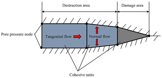
Figure 1.
The fluid flow schematic within a damaged unit.
Assuming that the fluid inside the cohesive unit is an incompressible Newtonian fluid, the calculation formula for the tangential flow is [34]:
where is the tangential flow rate, m3/s; ∇p is the pressure gradient along the length direction of the cohesive unit, Pa/m; is the fracture width, m; is the viscosity of the fracturing fluid, Pa s.
The normal leak-off loss on the upper and lower surfaces of the Cohesive unit can be described as [34]:
where and are the pore pressure at the upper and lower surfaces of the fracture, Pa; is the fluid pressure in the fracture, Pa; , are the fluid loss coefficients at the upper and lower surfaces, m3/(Pa·s); , are the normal volume flow of the upper and lower surfaces, respectively, m3/s.
The fluid mass conservation equation of the Cohesive unit is [35]:
where is the injection velocity of fracturing fluid, m3/s.
2.2. Criteria for Fracture Initiation and Propagation
At present, the commonly used finite element methods for numerical simulation of hydraulic fracturing include the finite element method based on the cohesive model and the extended finite element method [19]. The former is adopted in this paper, and the problem of infinite stress at the fracture tip of linear elastic fracture mechanics can be effectively avoided by inserting cohesive units between cells for describing nonlinear fracture problems. Cohesive elements provide a solution without refining the mesh, which can effectively reduce the number of meshes and improve the efficiency of operations [36].
2.2.1. Cohesive Unit Damage Model
The relationship between the tensile stress and the distance between the upper and lower surfaces is defined in the damage model of the Cohesive unit, and the definition of the damage evolution consists of two parts. A bilinear T-S criterion was proposed by V. Tomar [37]. As shown in Figure 2, the first part involves determining the effective displacement at full damage relative to the effective displacement at the onset of damage, or the energy dissipation due to failure. The second component defines the evolutionary nature of the damage variable D between initial and complete failure, which can be specified directly in the form of a table of effective displacement, effective displacement versus damage, by means of a linear or exponential softening law; the expression for the damage variable when the linear displacement expansion criterion is used is:
where is the maximum displacement of the unit; is the displacement of the unit opening; is the displacement of the unit starting damage.
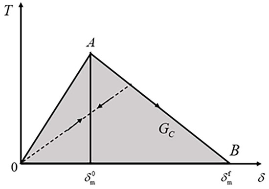
Figure 2.
Bilinear traction-separation curve.
The Cohesive unit uses stiffness degradation to describe the damage evolution of the unit.
where , , are the stresses obtained in the three directions of the cohesive unit according to the linear elastic deformation in the undamaged phase, respectively, and is the damage variable in Equation (4).
The T-S criterion is based on the tensile stress of the cohesive unit as the damage criterion; the unit is very stiff before the damage, the stress is proportional to the displacement and can be recovered after unloading, but when the tensile stress exceeds the tensile strength of the material, the stress it can withstand decays linearly with the increase in displacement and is not recoverable, which is more suitable for the fracture expansion process in hydraulic fracturing.
2.2.2. Cracking and Expansion of Cohesive Units
The following criteria are often used in the finite element method to determine fracture initiation: maximum positive stress criterion, maximum positive strain criterion, quadratic stress criterion and quadratic strain criterion [38,39]. In this study, after many attempts and simulations, it is considered that the maximum positive stress criterion is used, which is more stable as the basis for judging fracture initiation, and the calculation process is easy to converge and more compatible. That is, as soon as the stress in either direction of the unit reaches its critical stress, the unit starts to crack. The expression of the maximum positive stress criterion is as follows:
where refers to the maximum tensile stress that the unit can withstand in the vertical direction, i.e., the tensile strength of the reservoir, and and refer to the maximum shear stress that the unit can withstand in both directions, i.e., the shear strength of the reservoir.
For the expansion of composite fractures after fracture initiation, this paper adopts the B-K criterion, which is the criterion of critical energy release rate of crack expansion proposed by Benzeggagh and Kenane [40].
In Equation (7), , is the normal fracture critical strain energy release rate; , are the two tangential fracture critical energy release rates, respectively, and the B-K criterion considers ; η is a constant related to the properties of the material itself; is the composite fracture critical energy release rate.
Figure 3 shows a schematic diagram of the crack expansion of the cohesive unit. When the calculated energy release rate at the fracture tip node is greater than the B-K critical energy release rate, the current fracture tip node of the cohesive unit will unbind the bound part, and then the fracture will open and continue to expand along the next cohesive unit.
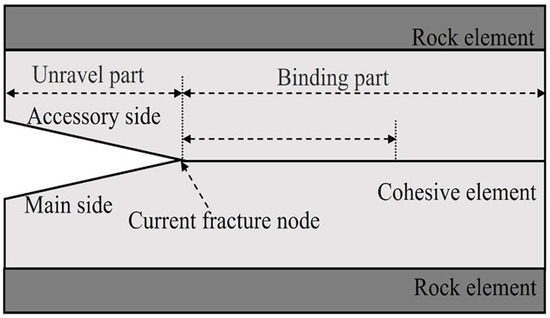
Figure 3.
Fracture propagation in the cohesive unit.
2.3. Fluid-Solid Coupling Control Equation
In the process of hydraulic fracturing, the fluid percolation pressure acting on the fracture wall increases continuously with the increase in pump pressure, which leads to the increase in fluid leak-off loss into the formation, resulting in the change in stress state in the rock pore space, and the change in stress in the rock will cause the change in parameters such as reservoir porosity and fluid percolation velocity, which in turn affects the change in pore pressure in the percolation field on the fracture wall. This relationship between fluid seepage and rock deformation is called fluid-solid coupling [41].
The rock skeleton stress balance equation for a unit body with volume and surface area is:
where σ and are the stress matrix and the imaginary strain rate matrix, respectively; , and are the surface force vector, the volume force vector and the imaginary velocity vector, respectively.
Fluid seepage is required to satisfy the continuity equation:
where J is the variation ratio of porous media body; is the fluid density; is the pore ratio; is the fluid percolation velocity; is the spatial vector.
Fluid flow in the cohesive unit satisfies Darcy’s law:
where is the permeability matrix of porous media; is the acceleration of gravity.
2.4. Fracture Wall Stress Distribution Model
This paper focuses on the upper propagation of the fracture. Generally, the model of numerical simulation calculation will be different from the actual situation, and some simplifications will be made [42]. To simplify the model, it is assumed that the upper and lower interlayer stresses in the reservoir are the same and symmetrically distributed along the centerline of the fracture. The model has the following assumptions: ①: the reservoir is an ideal thick oil formation, the rock is an ideal linear elastic material, and the ground stress is linearly distributed; ②: the fracture flanks are symmetrically distributed with the wellbore as the axis; ③: the fracturing fluid is an incompressible power-law fluid when it flows inside the fracture, and the two-dimensional flow of the fluid is considered; ④: the matrix permeability is low, and the leak-off of the fracturing fluid to the fracture wall is ignored; ⑤: the inertia effect is ignored.
According to the above assumptions, the stress distribution at the fracture wall is shown in Figure 4. Assuming that the reservoir thickness is and the height of fracture penetration into the barrier , let the minimum horizontal principal stress at the center of the fracture be , the minimum horizontal principal stress gradient be , the upper and lower reservoir interlayer stresses be the same, the reservoir interlayer stress difference be , the pressure drop of fracturing fluid gravity in the direction of the fracture height be , and the pressure drop generated by the artificial interlayer in the direction of the fracture height be .
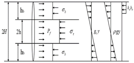
Figure 4.
Fracture wall stress distribution.
2.5. Mode Description
The numerical calculation model established in this paper is shown in Figure 5 for a three-dimensional model with dimensions of 40 m × 100 m × 100 m. The following assumptions are made for the model material: the reservoir is an ideal thick oil layer and the rock is an ideal linear elastic homogeneous material. The model is dissected into four areas, the thickness of both upper and lower layers as barriers is 20 m, the thickness of the middle area as the target reservoir is 60 m, and the height of the artificial barrier area formed by the diverting agents placement is 5 m. The (a) and (b) figures in Figure 6 show the profiles of the xoy plane and yoz plane, respectively. The perforation tunnel is chosen to be the center of the xoy plane, y is the direction of vertical principal stress, z is the direction of maximum horizontal principal stress, and x is the direction of minimum horizontal principal stress. The built-in Cohesive cell is embedded in the yoz plane as the fracture initiation and propagation path, perpendicular to the direction of the minimum horizontal principal stress, and the shot hole position is parallel to the direction of the maximum horizontal principal stress. The fracture propagation path and the basic morphology at different moments (t1, t2, t3) are depicted in Figure 6b. The type of solid element is C3D8P, which is a three-dimensional calculation unit with 8 nodes. It has the advantage of more accurate results for the displacement and the accuracy of the analysis will not be affected too much when there is distortion and deformation of the mesh. The mesh size of the numerical calculation model is chosen to be 2 m, and hexahedral elements are used completely in the mesh. For the three-dimensional geometric model, the mesh is first generated on the face and then stretched along the sweep path to obtain the three-dimensional mesh, and a total of 50,000 meshes are divided. The initial saturation of the target layer and the interlayer is set to 1; both are saturated seepage, and the constant pore pressure (20 MPa) is maintained at the left, right and upper and lower boundaries. The initial pore pressure is 20 MPa, the initial porosity of the reservoir is 0.3, and the initial porosity of the interlayer is 0.2. The fracturing fluid pumping discharge is set to 0.06 m3/s for 600 s, the fracturing fluid viscosity is 100 mPa·s, and the other initial values of the main calculated parameters are shown in Table 1.
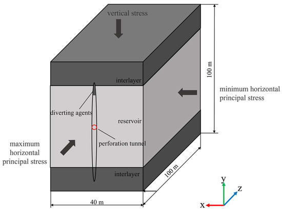
Figure 5.
Three-dimensional numerical calculation model.
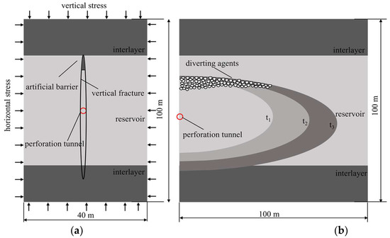
Figure 6.
Numerical calculation model (a): xoy profile chart, (b): yoz profile chart.

Table 1.
The rock mechanics parameters of the stratum.
Figure 7 shows the workflow of this study. The first step is to establish the fluid-solid coupling control equation on the basis of computational fluid dynamics. The second step is to establish a three-dimensional numerical calculation model considering artificial barriers in the finite element simulation software. On the basis of this model, combined with the previous laboratory experimental results, the calculation parameters are determined and the numerical simulation of fracture propagation is carried out. After the simulation, 3D fracture morphology data, model stress, and pore pressure clouds are extracted for parameter sensitivity analysis and discussion.
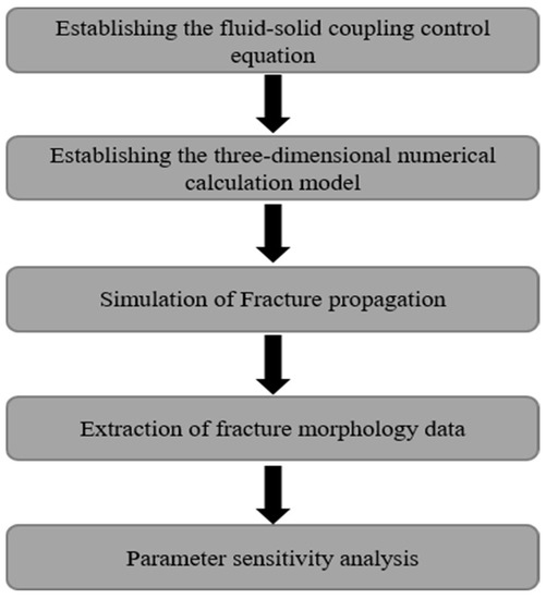
Figure 7.
Workflow of this study.
3. Result and Discussion
3.1. Young’s Modulus
The Young’s modulus of the reservoir rock is 30 GPa, the Young’s modulus of the interlayer is 28 GPa, and the Young’s modulus of the artificial barrier formed by diverting agents is 36, 34, 32 and 28 GPa, respectively. The values of other calculated parameters are shown in Table 2. The effect of different Young’s modulus of the artificial barrier on the fracture morphology is simulated and studied. Figure 8 shows the graphs of the fracture width and half-slit height under different Young’s modulus. It can be seen from Figure 8 that the larger the Young’s modulus of the artificial barrier, the more easily the fracture extends in the direction of the fracture height. Additionally, the change in the direction of the fracture width is not obvious and the range of the fracture width is distributed from 4.7 to 5.2 mm. However, there is a significant increase in the fracture width compared to the case without artificial barrier. It is analyzed that this is because the Young’s modulus will make the width of the fracture narrower, and the fracture height will increase correspondingly for a certain volume of injected fluid and leak-off. On the other hand, the higher the Young’s modulus of the artificial barrier, the more likely it is to develop high stresses at the fracture tip, and the more likely it is for the fracture to expand forward under the same tensile strength conditions.
Table 2.
The rock mechanics parameters of the stratum.
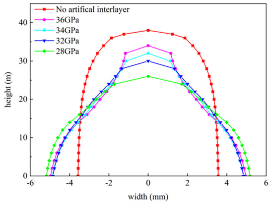
Figure 8.
Fracture morphology at different Young’s modulus of artificial barrier.
It is noteworthy that the fracture breaks through the area of each artificial barrier to extend into the area of the interlayer under the condition of Young’s modulus of the artificial barrier of 34 GPa or 36 GPa. Figure 8 shows that when the fracture penetrates the intersection and extends in the artificial barrier with a smaller Young’s modulus (28 GPa), the fracture width will increase slightly due to the sudden increase in the amount of leak−off when the fracture penetrates the dividing line between the artificial barrier and the interlayer, which leads to a slight increase in the fracture width and also an increase in the fracture height. Figure 9 shows the variation curve of pore pressure at the injection point with the injection time during the fracturing process, and the pore pressure variation when the fracture expands to the artificial barrier area is labeled. From Figure 9, it can be seen that the pore pressure at the injection point decreases slightly with the increase in Young’s modulus of the artificial barrier; the higher the pore pressure at the injection point, the greater the impediment to fracture extension. This indicates that the small Young’s modulus of the artificial barrier does have a hindering inhibiting effect on the vertical propagation of the fracture.
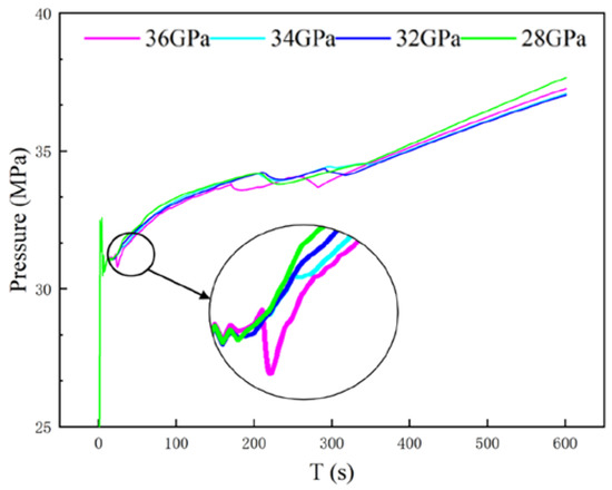
Figure 9.
Pore pressure at injection point with different Young’s modulus.
Figure 10 shows the stress distribution clouds of the fractured reservoir under different Young’s modulus conditions of the artificial barrier. It can be seen from the figure that the stress concentration area of the fracture changes with the increase in Young’s modulus, which is due to the different Young’s modulus of the artificial barrier, resulting in different fracture morphology. The larger Young’s modulus is the more unfavorable to control the fracture height.
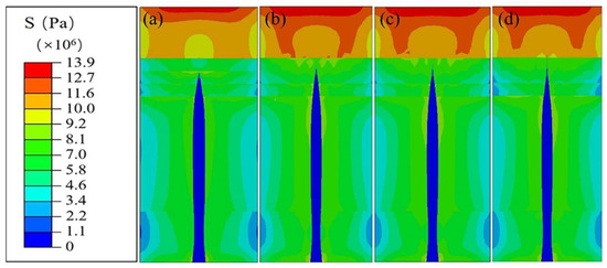
Figure 10.
Stress distribution cloud after fracturing under different Young’s modulus conditions: (a) 28 GPa, (b) 32 GPa, (c) 34 GPa, (d) 36 GPa.
Figure 11 shows the pore pressure distribution clouds of the reservoir after fracturing under different Young’s modulus conditions of the artificial barrier, from which it can be seen that: the reservoir pore pressure increases with the increase of Young’s modulus; the pore pressure shows a concentration phenomenon after fracturing; and a higher stress concentration zone is formed around the fracture.
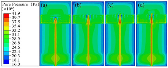
Figure 11.
Pore pressure distribution cloud after fracturing under different Young’s modulus conditions: (a) 28 GPa, (b) 32 GPa, (c) 34 GPa, (d) 36 GPa.
3.2. Leak-Off Coefficient
The size of the formation permeability is an important factor affecting fracture expansion, with low permeability reservoirs prone to fractures of a smaller horizontal extent and larger width, and the opposite for high permeability reservoirs [43]. The values of other calculated parameters are shown in Table 3. Since the fracture is extended on the preplaced cohesive cell, the fluid normal leak-off coefficient for the cohesive cell pore material defines the pressure-flux relationship between the intermediate nodes of the bonded cell and their adjacent surface nodes, and thus this coefficient can be interpreted as the cohesive bonded cell surface permeability of a finite material layer. Changing the leak-off coefficient of artificial barrier (1 × 10⁻⁷, 1 × 10⁻¹⁰, 1 × 10⁻¹³, 1 × 10⁻¹⁶) and studying the effect of the change in permeability of the artificial barrier on the fracture height, Figure 12 shows the graphs of the fracture width and half-slit height under different leak-off coefficients. With the decrease in the permeability of the artificial barrier, the morphology of the fracture changes greatly, and the change in fracture width direction is not significant. However, the control of permeability on the direction of fracture height of the fractured fracture is more obvious, in which the change in fracture height under the condition of maximum and minimum leak-off coefficient reaches about 10 m. When the leak-off coefficient of the artificial barrier is 1 × 10⁻¹⁶, the half fracture height is 16 m, when the leak-off coefficient increases to 1 × 10⁻⁷, the half fracture height increases by 10 m, but the width of the fracture decreases by about 0.2 m. This shows that the artificial barrier with low leak-off coefficient has significant control on the fracture height. Therefore, the placement of the artificial barrier with good sealing properties and a low leak-off coefficient is an important technical means to effectively control the fracture height.
Table 3.
The rock mechanics parameters of the stratum.
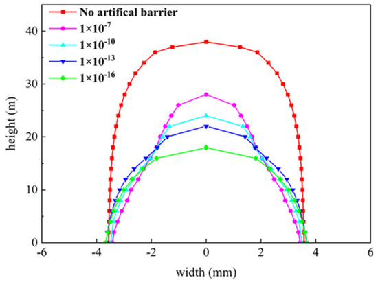
Figure 12.
Fracture morphology at different leak-off coefficient of artificial barrier.
Figure 13 shows the pore pressure distribution clouds of the fracture after fracturing under different leak-off coefficients, from which it can be seen that the formation pore pressure increases slightly with the decrease in the leak-off coefficient of the artificial barrier. When the leak-off coefficient is 1 × 10⁻⁷ and 1 × 10⁻¹⁰, the height of the fracture is smaller, but the fracture extension height above the injection point is greater than that of the leak-off coefficient of 1 × 10⁻¹³ and 1 × 10⁻¹⁶. The analysis suggests that because the total amount of fracturing fluid pumped remains unchanged, more fracturing fluid is transported to the lower end of the fracture due to the decrease in the leak-off coefficient of the artificial barrier, and the pore pressure at the lower end of the fracture is greater (c, d), thus achieving the purpose of controlling the upward expansion of the fracture.
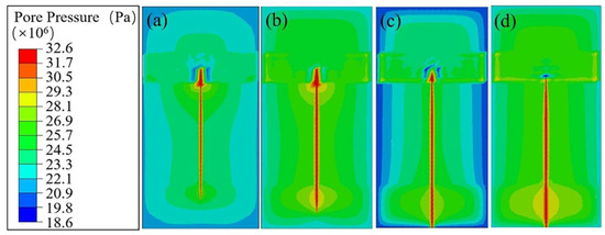
Figure 13.
Pore pressure distribution cloud after fracturing under different leak-off coefficient conditions: (a) 1 × 10⁻⁷, (b) 1 × 10⁻¹⁰, (c) 1 × 10⁻¹³, (d) 1 × 10⁻¹⁶.
3.3. Pumping Rate
In this section, the effect of different pumping rates on the fracture height extension in the presence of artificial barrier conditions is investigated. Since the model is plane strain, the pumping rates in this model are discounted accordingly to the field discharge, and five gradients are set: 0.04, 0.08, 0.1, 0.12, and 0.14 m3/s. Other parameters of the stratum are shown in Table 4, and the fracture morphology calculated by a numerical simulation is shown in Figure 14. With the increase in pumping rate, the fracture width and fracture height increase, and when the displacement increases from 0.12 m3/s to 0.14 m3/s, the extension in the fracture height direction is not obvious, and the fracture width continues to increase. The reason is that at this time, the factors affecting the fracture height are not only the size of pumping volume, but also the Young’s modulus and permeability of the artificial barrier.
Table 4.
The rock mechanics parameters of the stratum.
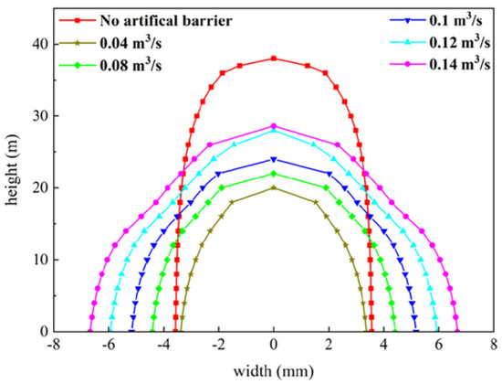
Figure 14.
Fracture morphology under different pumping rate.
Figure 15 shows the cloud plot of pore pressure distribution after fracturing under a different pumping rate. From the figure, it can be seen that the forming pore pressure increases with the increase in pumping rate, indicating that the displacement increases and the fracturing fluid leak−off loss also increases, while the pore pressure results in the pressure concentration phenomenon after fracturing, forming a high stress concentration zone around the fracture. When the pumping displacement is 0.04 m3/s, the lower end of the fracture is not enough to extend to the lower reservoir, and a high pore pressure concentration is formed at the lower end of the fracture.
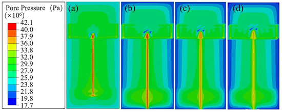
Figure 15.
Pore pressure distribution cloud after fracturing under different pumping rate: (a) 0.04 m3/s, (b) 0.08 m3/s, (c) 0.1 m3/s, (d) 0.12 m3/s.
Through the sensitivity analysis of the effects of the above three different parameters on the fracture morphology, the effects of Young’s modulus and the permeability of the artificial barrier on the fracture height were clarified, and the effects of pumping rates on the fracture propagation under the artificial barrier conditions were investigated. However, there are still some parts of this study that need to be improved. The three-dimensional numerical calculation model used in this study is homogeneous material and does not consider the effect of natural fractures and stratigraphic bedding on fracture morphology [44]. It should also be noted that the numerical simulation results of this study cannot be verified in the laboratory experiment. We will continue to refine this three-dimensional numerical model and add more different parameters to study the artificial barrier control fracture height technique, combined with microseismic monitoring techniques to verify the simulation results of this study.
4. Conclusions
In this study, a three-dimensional numerical calculation model of fracture propagation based on the bilinear traction-separation criterion is established, which considers the relationship between the mutual constraints and effects of fluid seepage and rock deformation. The effects of Young’s modulus, leak-off coefficient of the artificial barrier and pumping rate on fracture morphology are studied, and the following conclusions are drawn. The Young’s modulus of the artificial barrier has a significant effect on fracture morphology. Overall, the smaller the Young’s modulus of the artificial barrier, the smaller the fracture height formed by the fracturing construction, while the fracture width size does not vary much. When the Young’s modulus of the artificial barrier is 36 GPa, the half fracture height decreases by 4 m compared with the case without an artificial barrier. Similarly, the leak-off coefficient of the artificial barrier has great influence on fracture height, but has little influence on fracture width. When the leak-off coefficient decreases from 1 × 10⁻⁷ to 1 × 10⁻¹⁶, the half fracture height decreases by 10 m. The pore pressure cloud diagram shows that the artificial barrier with small leak-off coefficient can effectively organize the pressure in the fracture to transfer to the fracture end, so as to achieve the purpose of controlling the fracture height. The effect of pumping rates on fracture width and height are both more significant, which is different from the first two factors. With the increase in pumping rates, the height and width of the fracture increases. When the pumping rates increase from 0.04 m3/s to 0.12 m3/s, the half fracture height increases by 8 m, and when the pumping rate is 0.14 m3/s, the fracture height does not change much compared with 0.12 m3/s. In a subsequent study, we will continue to refine this three-dimensional numerical model to simulate the effects of other different properties of the artificial barrier on the fracture morphology and investigate the mechanism of the artificial barrier to control the fracture height. It will also be combined with field tests, such as using microseismic monitoring technology to verify the feasibility of artificial barrier control fracture height technology, and investigate the impact of artificial barriers formed by different types of diverting agents on oil and gas production.
Author Contributions
Writing—original manuscript, J.Z. and Y.Z.; methodology, Y.Z. and J.Z.; software, Y.Z. and L.Z.; writing—original draft preparation, J.J. and Y.F.; supervision, Y.W. and F.Z.; investigation, J.J.; data curation, Y.W. and G.Z.; formal analysis, Y.F. All authors have read and agreed to the published version of the manuscript.
Funding
This research was funded by the National Natural Science Foundation of China (No. 52174045).
Conflicts of Interest
The authors declare no conflict of interest.
References
- Ahmadi, Y.; Mohammadi, M.; Sedighi, M. Chapter 1—Introduction to Chemical Enhanced Oil Recovery. In Chemical Methods; Hemmati-Sarapardeh, A., Schaffie, M., Ranjbar, M., Dong, M., Li, Z., Eds.; Enhanced Oil Recovery Series; Gulf Professional Publishing: Houston, TX, USA, 2022; pp. 1–32. ISBN 978-0-12-821931-7. [Google Scholar]
- Mansouri, M.; Parhiz, M.; Bayati, B.; Ahmadi, Y. Preparation of Nickel Oxide Supported Zeolite Catalyst (NiO/Na-ZSm-5) for Asphaltene Adsorption: A Kinetic and Thermodynamic Study. Iran. J. Oil Gas Sci. Technol. 2021, 10, 63–89. [Google Scholar] [CrossRef]
- Ahmadi, Y. Relationship between Asphaltene Adsorption on the Surface of Nanoparticles and Asphaltene Precipitation Inhibition During Real Crude Oil Natural Depletion Tests. Iran. J. Oil Gas Sci. Technol. 2021, 10, 69–82. [Google Scholar] [CrossRef]
- Lin, H.; Tian, Y.; Sun, Z.; Zhou, F. Fracture Interference and Refracturing of Horizontal Wells. Processes 2022, 10, 899. [Google Scholar] [CrossRef]
- Zhu, D.; Wang, Y.; Cui, M.; Zhou, F.; Zhang, Y.; Liang, C.; Zou, H.; Yao, F. Effects of Spent Viscoelastic-Surfactant Acid Flow on Wormholes Propagation and Diverting Performance in Heterogeneous Carbonate Reservoir. Energy Rep. 2022, 8, 8321–8332. [Google Scholar] [CrossRef]
- Dong, R.; Wheeler, M.F.; Su, H.; Ma, K. Modeling Acid Fracturing Treatments in Heterogeneous Carbonate Reservoirs. In Proceedings of the SPE International Conference on Oilfield Chemistry, The Woodlands, TX, USA, 29 December 2021; OnePetro: Richardson, TX, USA, 2021. [Google Scholar]
- Zeng, H.; Jin, Y.; Wang, D.; Yu, B.; Zhang, W. Numerical Simulation on Hydraulic Fracture Height Growth across Layered Elastic–Plastic Shale Oil Reservoirs. Processes 2022, 10, 1453. [Google Scholar] [CrossRef]
- Merzoug, A.; Ellafi, A.; Rasouli, V.; Jabbari, H. Anisortopic Modeling of Hydraulic Fractures Height Growth in the Anadarko Basin. Appl. Mech. 2023, 4, 44–69. [Google Scholar] [CrossRef]
- Cao, Y.; He, Q.; Liu, C. Numerical Investigation of Fracture Morphology Characteristics in Heterogeneous Reservoirs. Processes 2022, 10, 2604. [Google Scholar] [CrossRef]
- Zhu, D.; Wang, Y.; Cui, M.; Zhou, F.; Wang, Y.; Liang, C.; Zou, H.; Yao, F. Acid System and Stimulation Efficiency of Multistage Acid Fracturing in Porous Carbonate Reservoirs. Processes 2022, 10, 1883. [Google Scholar] [CrossRef]
- Dong, R.; Wheeler, M.F.; Su, H.; Ma, K. Modeling Multistage Acid Fracturing Treatments in Carbonate Reservoirs. In Proceedings of the SPE Hydraulic Fracturing Technology Conference and Exhibition, Virtual, TX, USA, May 2021; OnePetro: Richardson, TX, USA, 2021. [Google Scholar]
- Dong, R.; Wheeler, M.F.; Su, H.; Ma, K. Modeling Acid Fracturing Treatments with Multi-Stage Alternating Injection of Pad and Acid Fluids. In Proceedings of the SPE Reservoir Simulation Conference, On-Demand, TX, USA, October 2021; OnePetro: Richardson, TX, USA, 2021. [Google Scholar]
- Nguyen, H.X.; Larson, D.B. Fracture Height Containment by Creating an Artificial Barrier With a New Additive. In Proceedings of the SPE Annual Technical Conference and Exhibition, San Francisco, CA, USA, October 1983; OnePetro: Richardson, TX, USA, 1983. [Google Scholar]
- Morales, R.; Fragachan, F.E.; Prado, E.; Santillan, J. Production Optimization by an Artificial Control Of Fracture Height Growth. In Proceedings of the SPE European Formation Damage Conference, The Hague, The Netherlands, June 1997; OnePetro: Richardson, TX, USA, 1997. [Google Scholar]
- Arp, M.E.; Hilton, R.E. Case History Study of Fracture Height Containment in East Texas. In Proceedings of the SPE East Texas Regional Meeting, Tyler, TX, USA, April 1986; OnePetro: Richardson, TX, USA, 1986. [Google Scholar]
- Mukherjee, H.; Paoli, B.F.; McDonald, T.; Cartaya, H.; Anderson, J.A. Successful Control of Fracture Height Growth by Placement of Artificial Barrier. SPE Prod. Facil. 1995, 10, 89–95. [Google Scholar] [CrossRef]
- Khodaverdian, M.; McElfresh, P. Hydraulic Fracturing Stimulation in Poorly Consolidated Sand: Mechanisms and Consequences. In Proceedings of the SPE Annual Technical Conference and Exhibition, Dallas, TX, USA, October 2000; OnePetro: Richardson, TX, USA, 2000. [Google Scholar]
- Peng, S.; Zhang, X.; Tang, X.; Xu, J.; Jiao, F.; He, M. Experimental Investigation of Non-Linear Seepage Characteristics in Rock Discontinuities and Morphology of the Shear Section in the Shear Process. Processes 2022, 10, 2625. [Google Scholar] [CrossRef]
- Carrier, B.; Granet, S. Numerical Modeling of Hydraulic Fracture Problem in Permeable Medium Using Cohesive Zone Model. Eng. Fract. Mech. 2012, 79, 312–328. [Google Scholar] [CrossRef]
- Yan, J.I.N.; Xu-dong, Z.; Mian, C. Initiation Pressure Models for Hydraulic Fracturing of Vertical Wells in Naturally Fractured Formation. Acta Pet. Sin. 2005, 26, 113. [Google Scholar] [CrossRef]
- Adachi, J.; Siebrits, E.; Peirce, A.; Desroches, J. Computer Simulation of Hydraulic Fractures. Int. J. Rock Mech. Min. Sci. 2007, 44, 739–757. [Google Scholar] [CrossRef]
- Xu, B.; Liu, Y.; Wang, Y.; Yang, G.; Yu, Q.; Wang, F. A New Method and Application of Full 3D Numerical Simulation for Hydraulic Fracturing Horizontal Fracture. Energies 2019, 12, 48. [Google Scholar] [CrossRef]
- Simoni, L.; Secchi, S. Cohesive Fracture Mechanics for a Multi-phase Porous Medium. Eng. Comput. 2003, 20, 675–698. [Google Scholar] [CrossRef]
- Lecampion, B. An Extended Finite Element Method for Hydraulic Fracture Problems. Commun. Numer. Methods Eng. 2009, 25, 121–133. [Google Scholar] [CrossRef]
- Chen, Z.; Bunger, A.P.; Zhang, X.; Jeffrey, R.G. Cohesive Zone Finite Element-Based Modeling of Hydraulic Fractures. Acta Mech. Solida Sin. 2009, 22, 443–452. [Google Scholar] [CrossRef]
- Sun, S.; Zhou, M.; Lu, W.; Davarpanah, A. Application of Symmetry Law in Numerical Modeling of Hydraulic Fracturing by Finite Element Method. Symmetry 2020, 12, 1122. [Google Scholar] [CrossRef]
- Wan, B.; Liu, Y.; Zhang, B.; Luo, S.; Wei, L.; Li, L.; He, J. Investigation of the Vertical Propagation Pattern of the 3D Hydraulic Fracture under the Influence of Interlayer Heterogeneity. Processes 2022, 10, 2449. [Google Scholar] [CrossRef]
- Zhao, Y.; Wang, L.; Ma, K.; Zhang, F. Numerical Simulation of Hydraulic Fracturing and Penetration Law in Continental Shale Reservoirs. Processes 2022, 10, 2364. [Google Scholar] [CrossRef]
- Behnia, M.; Goshtasbi, K.; Zhang, G.; Mirzeinaly Yazdi, S.H. Numerical Modeling of Hydraulic Fracture Propagation and Reorientation. Eur. J. Environ. Civ. Eng. 2015, 19, 152–167. [Google Scholar] [CrossRef]
- Dahi Taleghani, A.; Gonzalez-Chavez, M.; Yu, H.; Asala, H. Numerical Simulation of Hydraulic Fracture Propagation in Naturally Fractured Formations Using the Cohesive Zone Model. J. Pet. Sci. Eng. 2018, 165, 42–57. [Google Scholar] [CrossRef]
- Li, J.; Dong, S.; Hua, W.; Li, X.; Pan, X. Numerical Investigation of Hydraulic Fracture Propagation Based on Cohesive Zone Model in Naturally Fractured Formations. Processes 2019, 7, 28. [Google Scholar] [CrossRef]
- Putra, R.U.; Basri, H.; Prakoso, A.T.; Chandra, H.; Ammarullah, M.I.; Akbar, I.; Syahrom, A.; Kamarul, T. Level of Activity Changes Increases the Fatigue Life of the Porous Magnesium Scaffold, as Observed in Dynamic Immersion Tests, over Time. Sustainability 2023, 15, 823. [Google Scholar] [CrossRef]
- Tauviqirrahman, M.; Jamari, J.; Susilowati, S.; Pujiastuti, C.; Setiyana, B.; Pasaribu, A.H.; Ammarullah, M.I. Performance Comparison of Newtonian and Non-Newtonian Fluid on a Heterogeneous Slip/No-Slip Journal Bearing System Based on CFD-FSI Method. Fluids 2022, 7, 225. [Google Scholar] [CrossRef]
- Economides, M.J.; Nolte, K.G. Reservoir Stimulation; Prentice Hall: Englewood Cliffs, NJ, USA, 1989; Volume 2. [Google Scholar]
- Peirce, A.; Detournay, E. An Implicit Level Set Method for Modeling Hydraulically Driven Fractures. Comput. Methods Appl. Mech. Eng. 2008, 197, 2858–2885. [Google Scholar] [CrossRef]
- Neves, L.F.R.; Campilho, R.D.S.G.; Sánchez-Arce, I.J.; Madani, K.; Prakash, C. Numerical Modelling and Validation of Mixed-Mode Fracture Tests to Adhesive Joints Using J-Integral Concepts. Processes 2022, 10, 2730. [Google Scholar] [CrossRef]
- Tomar, V.; Zhai, J.; Zhou, M. Bounds for Element Size in a Variable Stiffness Cohesive Finite Element Model. Int. J. Numer. Methods Eng. 2004, 61, 1894–1920. [Google Scholar] [CrossRef]
- Campilho, R.D.S.G.; de Moura, M.F.S.F.; Domingues, J.J.M.S. Modelling Single and Double-Lap Repairs on Composite Materials. Compos. Sci. Technol. 2005, 65, 1948–1958. [Google Scholar] [CrossRef]
- Camanho, P.P.; Davila, C.G. Mixed-Mode Decohesion Finite Elements for the Simulation of Delamination in Composite Materials; No. NAS 1.15: 211737; NASA Center for AeroSpace Information: Hanover, MD, USA, 2002. Available online: https://ntrs.nasa.gov/citations/20020053651 (accessed on 10 December 2022).
- Benzeggagh, M.L.; Kenane, M. Measurement of Mixed-Mode Delamination Fracture Toughness of Unidirectional Glass/Epoxy Composites with Mixed-Mode Bending Apparatus. Compos. Sci. Technol. 1996, 56, 439–449. [Google Scholar] [CrossRef]
- Yang, K.; Gao, D. Numerical Simulation of Hydraulic Fracturing Process with Consideration of Fluid–Solid Interaction in Shale Rock. J. Nat. Gas Sci. Eng. 2022, 102, 104580. [Google Scholar] [CrossRef]
- Dong, R.; Wheeler, M.F.; Ma, K.; Su, H. A 3D Acid Transport Model for Acid Fracturing Treatments With Viscous Fingering. In Proceedings of the SPE Annual Technical Conference and Exhibition, Virtual, TX, USA, October 2020; OnePetro: Richardson, TX, USA, 2020. [Google Scholar]
- Ren, L.; Lin, R.; Zhao, J.; Yang, K.; Hu, Y.; Wang, X. Simultaneous Hydraulic Fracturing of Ultra-Low Permeability Sandstone Reservoirs in China: Mechanism and Its Field Test. J. Cent. South Univ. 2015, 22, 1427–1436. [Google Scholar] [CrossRef]
- Wu, J.; Li, X.; Wang, Y. Insight into the Effect of Natural Fracture Density in a Shale Reservoir on Hydraulic Fracture Propagation: Physical Model Testing. Energies 2023, 16, 612. [Google Scholar] [CrossRef]
Disclaimer/Publisher’s Note: The statements, opinions and data contained in all publications are solely those of the individual author(s) and contributor(s) and not of MDPI and/or the editor(s). MDPI and/or the editor(s) disclaim responsibility for any injury to people or property resulting from any ideas, methods, instructions or products referred to in the content. |
© 2023 by the authors. Licensee MDPI, Basel, Switzerland. This article is an open access article distributed under the terms and conditions of the Creative Commons Attribution (CC BY) license (https://creativecommons.org/licenses/by/4.0/).