Exact Analytical Relations for the Average Release Time in Diffusional Drug Release

Abstract

Although analytical solutions for the problem of diffusion-controlled drug release from uniform formulations of simple geometries, like slabs, spheres, or cylinders, are well known, corresponding exact expressions for the average release times are not widely used. However, such exact analytical formulae are very simple and useful. When the drug is initially distributed homogeneously within the matrix, the average time of release from a sphere of radius R is $t_{av}=(1/15)R^2/D$ and from a slab of thickness L is $t_{av}=(1/12)L^2/D$, where D is the corresponding drug diffusion coefficient. Regarding cylindrical tablets of height H and radius R, simple analytical expressions are obtained in the two opposite limits of either very long ($H\gg R$) or very short ($H\ll R$) cylinders. In the former case, of practically radial release, the average release time is $t_{av}=(1/8)R^2/D$, while in the latter case the same result as that of a slab with thickness H is recovered, $t_{av}=(1/12)H^2/D$, as expected. These simple and exact relations are useful not only for an estimate of the average release time from a drug carrier device when diffusion is the dominant mechanism of drug delivery, but also for the experimental determination of the drug diffusion coefficient in a release system of interest through the measured release profile, given the mean squared size of the formulation.

1. Introduction

For the proper design of a pharmaceutical dosage form it is very important to control the time scale at which the bioactive compound is delivered. Accurate theoretical calculations, including mathematical models with explicit analytical expressions or numerical computations, can greatly contribute towards this goal. There are many theoretical investigations aiming to estimate the properties of drug release profiles and several review articles discuss these efforts; see, for example, [1,2]. Other reviews focus on mathematical modeling of drug delivery from specific type of carriers, like microspheres [3], hydrogels [4], bulk degrading polymers [5], supramolecular systems [6], or diffusion-controlled formulations in the presence of a size distribution [7].

Depending on the physical mechanism that dominates the release process in a particular case, various analytical methods or numerical simulations have been proposed in order to investigate the release characteristics. Therefore, different models have been developed which describe situations ranging from pure diffusion [8,9,10,11,12,13,14,15,16,17] to reaction–diffusion systems [18,19,20,21,22,23,24], to hydrogel swelling [25,26,27], or to kinetically limited release [28,29].

The drug carriers used in relevant experiments usually have simple geometrical shapes, like thin films or slabs [30,31,32,33,34,35], spheres or pellets [36,37,38,39,40,41], and cylindrical tablets or fibers [42,43]. In the particular case of diffusion-controlled release from such geometries, exact analytical formulae concerning the fractional release profiles are well known, when the drug is homogeneously distributed initially and the formulation is uniform [44], or it has a core–shell structure [45].

However, the aforementioned analytical expressions describing the time dependence of fractional release are in the form of sums of infinite series and thus they are somehow intractable for practical use. As a result, simpler empirical functions have been suggested as approximate expressions in order to describe a part of the release kinetics or the complete release profile. The release profile refers to the variation with time of the cumulative relative amount of released drug $M_t/M_{\infty }$, where $M_t$ is the amount of drug that has escaped from the formulation up to time t and $M_{\infty }$ denotes the total amount of initially loaded drug which is expected to be fully released after a very long (“infinite”) time. Widely used approximate empirical functions are the Peppas power law, $M_t/M_{\infty }=k{t}^n$ [46,47], and the stretched exponential (known also as Weibull function), $M_t/M_{\infty }=1-e^{-{(t/{\tau }_s)}^b}$ [48,49,50,51]. The k and n in the former case, and the b and ${\tau }_s$ in the latter are free parameters to be determined through fitting with the obtained release profile. More recently, another two-parameter empirical function has been proposed, which interpolates between the short-time and long-time behavior of the exact analytical solution of $M_t/M_{\infty }$ [52,53].

Here, instead of focusing on the entire temporal profile of the fractional release $\frac{M_t}{M_{\infty }}\left(t\right)$, a single value characterizing this time dependence is examined, namely the average release time $t_{av}$. The purpose of this work is to discuss simple expressions for the average release time, in the case of diffusion-controlled drug release from different matrix geometries, like spheres, slabs, or cylinders. The exact relations considered here are directly derived through the known analytical solutions of the corresponding diffusion equation, in the form of infinite series. The average release time is given as a function of the parameters of the release system, that is, the size of the formulation and the drug diffusion coefficient, through very simple analytical formulae in the cases of spheres and slabs, as well as in the limiting cases of either very long cylindrical rods or very short cylinders (flat discs).

Contrary to the inconvenient infinite series form of the complete release profiles, the exact simple relations discussed here regarding the average release times can be efficiently used for practical applications:

• To directly determine the release time scale during the design of a drug delivery device.
• To obtain the drug diffusion coefficient within the formulation, through an experimental estimate of the average release time $t_{av}$ by the measured release profile, given the size of the drug carrier (or the average squared size when there is a distribution of carrier sizes).

Concerning the latter application, the average release time $t_{av}$ can be easily derived experimentally through the area under the plot of the quantity $1-\frac{M_t}{M_{\infty }}$ or, even simpler in many cases, through the time instant at which a particular fraction of the drug, around 65%, has been released (see Section 3 below).

2. Methods

At the beginning of a diffusional release process there is not any drug released yet, while at very long times the whole amount of drug enclosed in the formulation has been released. Therefore, the fractional release $\frac{M_t}{M_{\infty }}\left(t\right)$ varies from 0 to 1 as time increases from zero to infinity. The complement fractional release

$$1-\frac{M_t}{M_{\infty }}$$

(1)

which expresses the relative amount of drug still remaining within the formulation, is then varied from 1 to 0 as time increases. As a result, the area under the plot depicting the variation of this last quantity with time, i.e. the simple integral of the complement fractional release over time, can be used to provide the characteristic average time of the release process [24,52,53]:

$$t_{av}={\int }_0^{\infty }\left(1-\frac{M_t}{M_{\infty }}\right)dt$$

(2)

The method of calculation of the average release time through Equation (2) is identical to the procedure used to obtain the average decay time characterizing an exponential decrease $e^{-kt}$ from 1 to 0. In the latter case, $t_{av}^{exp}={\int }_0^{\infty }{e}^{-kt}dt=1/k$, where k is the decay rate of the exponential decrease. Correspondingly, the average time in a process described by a stretched exponential decay from 1 to 0, see Equation (9) of Ref. [11] or Equation (12) of Ref. [52], is obtained in a similar way through an integral over time such as that of Equation (2). The difference here, in the context of drug delivery, is that the complement fractional release $1-\frac{M_t}{M_{\infty }}$ is not decaying exponentially or through a stretched exponential (even though it can be approximated rather well by the Weibull function [11,45,48,49]), but in a more complicated manner as an infinite sum of exponentials, see for example Equations (5), (12) and (21) below. However, it still decays from 1 to 0. This is a necessary requirement for the applicability of Equation (2) in order to provide the characteristic average time of the process.

As we see in Section 3.1, Section 3.2 and Section 3.3.1, in the case of diffusional drug delivery, at times equal to the corresponding average release time, i.e. for $t=t_{av}$, the complement fractional release has decayed to around 33% for spherical formulations, around 36% for slabs, and around 34% for long cylindrical rods, in comparison to the $1/e\approx 37\%$ decay of an exponential decrease at $t=t_{av}^{exp}=1/k$. This means that the average release time of a diffusion-controlled drug delivery process is moved towards larger reductions of the fractional amount of drug still remaining within the formulation, as compared to the case of a first order (exponential) release.

Through the exact analytical solutions of the diffusion equation in different drug carrier geometries, the integral of Equation (2) is explicitly calculated in Section 3, resulting in exact and simple relations for the corresponding average release times. For convenience, dimensionless time units will be used in the derivation. Then, the real units, which carry the dependence on the parameters of the system, will be restored at the end of the calculation.

3. Results

The average release times discussed below concern situations where diffusion is the dominant drug delivery mechanism. Other assumptions regarding the validity of the presented results are that (i) spatially uniform devices are considered, (ii) initially the bioactive substance is distributed homogeneously, i.e. its concentration is constant across the formulation, and (iii) sink boundary conditions are applied at the external surfaces of the drug carriers. The drug diffusion coefficient within the matrix is denoted by D. Average release times from matrices in the form of spheres, slabs, and cylinders are presented in Section 3.1, Section 3.2 and Section 3.3, respectively.

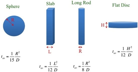
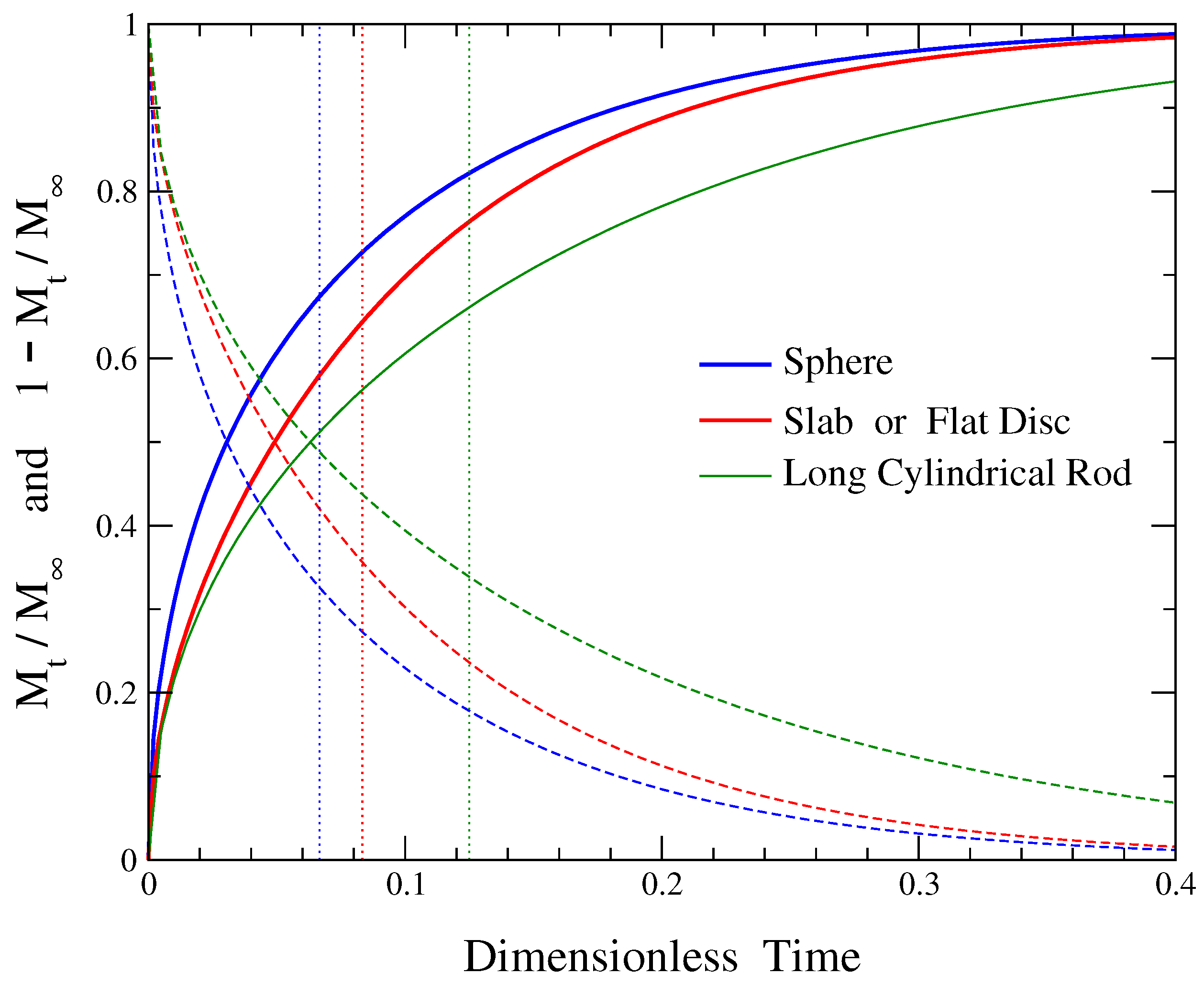
3.1. Release from a Sphere of Radius R

Considering homogeneously loaded and uniform spherical formulations or pellets of radius R, the solution of diffusion equation yields for the fractional release profile [8,11,44]

$$\frac{M_t}{M_{\infty }}=1-\frac{6}{{\pi }^2}\sum _{n=1}^{\infty }\frac{1}{n^2}{e}^{-n^2{\pi }^{2}Dt/R^2}$$

(3)

Using the dimensionless time [11]

$$\tau =\frac{D}{R^2}t$$

(4)

the complement fractional release is

$$1-\frac{M_t}{M_{\infty }}=\frac{6}{{\pi }^2}\sum _{n=1}^{\infty }\frac{1}{n^2}{e}^{-n^2{\pi }^2\tau }$$

(5)

The dimensionless average time, obtained from Equation (2), is

$${\tau }_{av}={\int }_0^{\infty }\left(1-\frac{M_t}{M_{\infty }}\right)d\tau =\frac{6}{{\pi }^2}\sum _{n=1}^{\infty }\frac{1}{n^2}{\int }_0^{\infty }{e}^{-n^2{\pi }^2\tau }d\tau =\frac{6}{{\pi }^4}\sum _{n=1}^{\infty }\frac{1}{n^4}$$

(6)

Taking into account the value of the sum

$$\sum _{n=1}^{\infty }\frac{1}{n^4}=\frac{{\pi }^4}{90}$$

(7)

the dimensionless average time is derived

$${\tau }_{av}=\frac{1}{15}$$

(8)

Returning now in real time units, from Equation (4) we obtain $t_{av}=(R^2/D){\tau }_{av}$ and, thus,

$$t_{av}=\frac{1}{15}\frac{R^2}{D}$$

(9)

is the resulting average release time from a spherical device.

Figure 1 depicts the fractional release profile for a diffusional release from a sphere (increasing, blue continuous line), given by Equation (3), and its complement fractional release (decreasing blue dashed line), provided by Equation (5), both as functions of the dimensionless time $\tau$ of Equation (4). The value of the average release time ${\tau }_{av}$, Equation (8), is indicated by the blue vertical dotted line in this figure. The average release time equals the area under the plot of the complement fractional release $1-M_t/M_{\infty }$ versus time, which is shown by the dashed blue line. At the time instant equal to the average release time, $\tau =1/15\approx 0.0667$, the corresponding value of the fractional release $M_t/M_{\infty }$ is around 0.67, i.e., approximately 67% of the drug has been released. The complement fractional release at that time has decayed to around 33%, providing the corresponding percentage of the initially loaded drug that is still remaining within the matrix at $\tau ={\tau }_{av}$.

3.2. Release from a Slab of Thickness L

In the case of diffusion-controlled release from a uniform thin film or slab of thickness L with a homogeneous initial drug distribution, the fractional release equals [8,12,44]

$$\frac{M_t}{M_{\infty }}=1-\frac{8}{{\pi }^2}\sum _{n=0}^{\infty }\frac{1}{{(2n+1)}^2}{e}^{-{(2n+1)}^2{\pi }^{2}Dt/L^2}$$

(10)

Now, the dimensionless time is defined as [12]

$$\tau =\frac{D}{L^2}t$$

(11)

and the corresponding complement fractional release is

$$1-\frac{M_t}{M_{\infty }}=\frac{8}{{\pi }^2}\sum _{n=0}^{\infty }\frac{1}{{(2n+1)}^2}{e}^{-{(2n+1)}^2{\pi }^2\tau }$$

(12)

As a result, the dimensionless average time from Equation (2) is

$${\tau }_{av}={\int }_0^{\infty }\left(1-\frac{M_t}{M_{\infty }}\right)d\tau =\frac{8}{{\pi }^2}\sum _{n=0}^{\infty }\frac{1}{{(2n+1)}^2}{\int }_0^{\infty }{e}^{-{(2n+1)}^2{\pi }^2\tau }d\tau =\frac{8}{{\pi }^4}\sum _{n=0}^{\infty }\frac{1}{{(2n+1)}^4}$$

(13)

Using the value of the infinite sum

$$\sum _{n=0}^{\infty }\frac{1}{{(2n+1)}^4}=\frac{{\pi }^4}{96}$$

(14)

the dimensionless average time is obtained from Equation (13)

$${\tau }_{av}=\frac{1}{12}$$

(15)

Restoring real units, from Equation (11) we have $t_{av}=(L^2/D){\tau }_{av}$ and, therefore, the average release time from a slab is equal to

$$t_{av}=\frac{1}{12}\frac{L^2}{D}$$

(16)

This result has also been obtained in Ref. [52] in terms of the longest relaxation time appearing in the exponentials of Equation (10).

Figure 1 shows with red lines the dependence of the fractional release and the complement fractional release, obtained through Equations (10) and (12), respectively, on the dimensionless time $\tau$ of Equation (11). The area under the plot of $1-M_t/M_{\infty }$ versus time, Equation (12), corresponds to the average release time ${\tau }_{av}$. Its exact value is provided by Equation (15) and it is depicted by the vertical red dotted line in Figure 1. The value of fractional release at $\tau ={\tau }_{av}=1/12\approx 0.0833$ in this case is $M_t/M_{\infty }\approx 0.64$, indicating that the cumulative amount of drug released up to this time is around 64%. The complement fractional release has decayed to around 36% at that time.

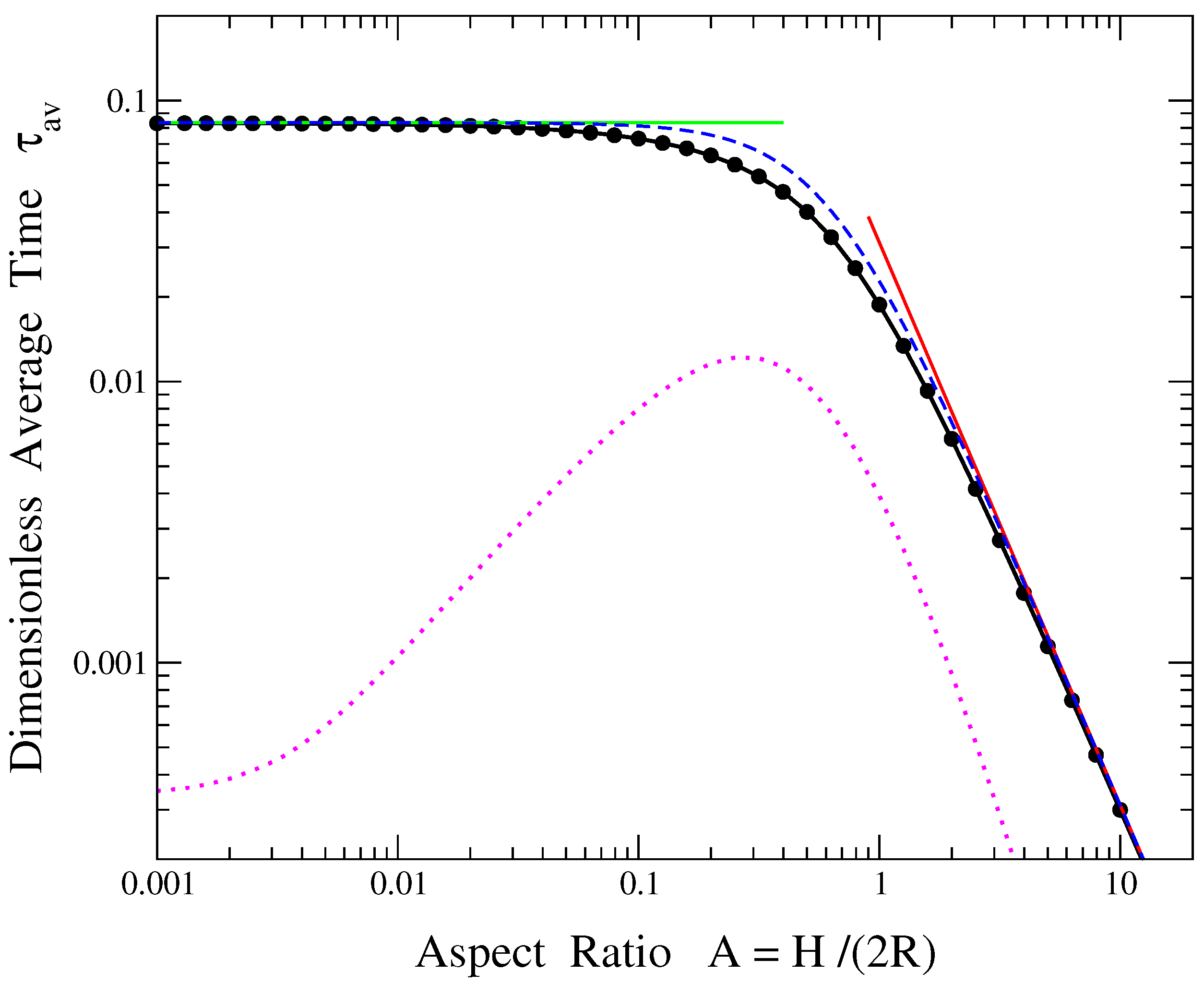
3.3. Release from a Cylinder of Height H and Radius R

Finally, diffusional release from a uniform cylindrical tablet of height H and radius R is considered. When the initial drug loading is homogenous, then the fractional release profile is given by [44,48,54]

$$\frac{M_t}{M_{\infty }}=1-\frac{32}{{\pi }^2}\sum _{m=1}^{\infty }\frac{1}{{\lambda }_m^2}{e}^{-{\lambda }_m^{2}Dt/R^2}\sum _{n=0}^{\infty }\frac{1}{{(2n+1)}^2}{e}^{-{(2n+1)}^2{\pi }^{2}Dt/H^2}$$

(17)

where ${\lambda }_m$ represents the mth root of the zero-order Bessel function $J_0\left(x\right)$ and the first sum over m corresponds to a sum over all roots of the equation $J_0\left(x\right)=0$. This means that ${\lambda }_1\approx 2.4048$, ${\lambda }_2\approx 5.5201$, ${\lambda }_3\approx 8.6537$, ${\lambda }_4\approx 11.7915$, etc. [55].

Considering the aspect ratio A of the cylinder as the ratio of its length (height) over its diameter $2R$

$$A=\frac{H}{2R}$$

(18)

and the dimensionless time

$$\tau =\frac{D}{H^2}t$$

(19)

then the solution of the diffusion equation given by Equation (17) can be written as

$$\frac{M_t}{M_{\infty }}=1-\frac{32}{{\pi }^2}\sum _{m=1}^{\infty }\sum _{n=0}^{\infty }\frac{1}{{\lambda }_m^2{(2n+1)}^2}{e}^{-[4A^2{\lambda }_m^2+{(2n+1)}^2{\pi }^2]\tau }$$

(20)

In this case, the complement fractional release is

$$1-\frac{M_t}{M_{\infty }}=\frac{32}{{\pi }^2}\sum _{m=1}^{\infty }\sum _{n=0}^{\infty }\frac{1}{{\lambda }_m^2{(2n+1)}^2}{e}^{-[4A^2{\lambda }_m^2+{(2n+1)}^2{\pi }^2]\tau }$$

(21)

and the corresponding dimensionless average time is

$${\tau }_{av}={\int }_0^{\infty }\left(1-\frac{M_t}{M_{\infty }}\right)d\tau =\frac{32}{{\pi }^2}\sum _{m=1}^{\infty }\sum _{n=0}^{\infty }\frac{1}{{\lambda }_m^2{(2n+1)}^2[4A^2{\lambda }_m^2+{(2n+1)}^2{\pi }^2]}$$

(22)

Due to the square bracket term in the denominator, the coupled double sum in the last equation cannot be easily evaluated towards a simpler expression. However, in the two limiting cases of either very long cylinders, where $H\gg R$ and A tends to infinity, or very short cylinders, where $H\ll R$ and A tends to zero, one of the two terms within the square brackets in the denominator of Equation (22) can be ignored as negligible in comparison to the other one. Then, the double sum is decoupled. In these situations simple analytical expressions are derived, as discussed in Section 3.3.1 and Section 3.3.2.

In the general case of an arbitrary value of the aspect ratio A, the exact result of ${\tau }_{av}$ given by Equation (22) can be computed through a numerical evaluation of the coupled double sum. Such a numerical calculation of ${\tau }_{av}$ versus A is shown in Figure 2 by the line-connected black circles. The simple analytical expressions valid in the two aforementioned limits of $H\ll R\Rightarrow A\ll 1$ or $H\gg R\Rightarrow A\gg 1$, see Equations (38) and (29) below, are represented by the continuous green and red lines, respectively. It can be seen from Figure 2 that the former expression describes rather well the numerically calculated values of ${\tau }_{av}$ when the aspect ratio is smaller than a value of $A\approx 0.05$, while the latter one provides an accurate approximation of the average release time when the aspect ratio is larger than a value of $A\approx 5$. For intermediate values of A, a simple formula interpolating between the corresponding analytical relations at the two opposite limits, Equations (38) and (29), respectively, can be used as a crude approximation of the average release time:

$${\tau }_{av}\approx \frac{1}{4(8A^2+3)}$$

(23)

This interpolating expression is also shown in Figure 2 by the blue dashed curve. It provides a rough approximation of ${\tau }_{av}$ in the region $0.05\lesssim A\lesssim 5$, i.e., when the ratio of a cylinder’s length over its radius, $H/R=2A$, is within the range $0.1\lesssim H/R\lesssim 10$. Note that the approximate estimate of $t_{av}$ from the simpler Equation (23) is always larger than its exact value given by Equation (22), i.e., it overestimates the average release time. The magenta dotted line in Figure 2 depicts the difference between the approximate formula of ${\tau }_{av}$ in Equation (23) and the numerically obtained exact double sum of Equation (22), i.e., the difference between the blue dashed and black solid curves of the figure. It should be mentioned however that, even though this difference seems to be small, the values of ${\tau }_{av}$ are small too. As a result, the relative difference exceeds 10% in the region $0.2\lesssim H/R\lesssim 6$, while its maximum value is around 24% when $H/R\approx 1$.

The average release time in real units is given by $t_{av}=(H^2/D){\tau }_{av}$, see Equation (19); thus, Equation (22) implies

$$t_{av}=\frac{32}{{\pi }^2}\left(\sum _{m=1}^{\infty }\sum _{n=0}^{\infty }\frac{1}{{\lambda }_m^2{(2n+1)}^2[4A^2{\lambda }_m^2+{(2n+1)}^2{\pi }^2]}\right)\frac{H^2}{D}$$

(24)

Note that in this relation the geometrical dimensions of the cylindrical drug carrier appear not only in the numerator $H^2$ of the last fraction, but also in the square bracket term within the double sum through the aspect ratio A. Taking into account the dependence of the double sum on $4A^2$, in combination with Equation (18), one sees that the term within the large parentheses of the last equation is a function of ${(H/R)}^2$.

Correspondingly, the simpler Equation (23) yields in real units

$$t_{av}\approx \frac{1}{4(8A^2+3)}\frac{H^2}{D}=\frac{1}{4[2{(H/R)}^2+3]}\frac{H^2}{D}$$

(25)

which can be used as a rough approximation of the average release time in cylindrical tablets with a length over radius ratio $H/R$ ranging from ∼0.1 up to ∼10.

3.3.1. Very Long Cylinders ($H\gg R$)

This situation corresponds to long cylindrical rods of radius R. Now, the aspect ratio A of Equation (18) tends to infinity and thus the first term $4A^2{\lambda }_m^2$ dominates inside the square brackets of the denominator of Equation (22). Thus, ignoring the corresponding second term, the dimensionless average time is given in this limit by

$${\tau }_{av}=\frac{32}{{\pi }^2}\sum _{m=1}^{\infty }\sum _{n=0}^{\infty }\frac{1}{4A^2{\lambda }_m^4{(2n+1)}^2}=\frac{8}{A^2{\pi }^2}\sum _{m=1}^{\infty }\frac{1}{{\lambda }_m^4}\sum _{n=0}^{\infty }\frac{1}{{(2n+1)}^2}$$

(26)

Taking into account that, for the roots ${\lambda }_m$ of $J_0\left(x\right)$, it is

$$\sum _{m=1}^{\infty }\frac{1}{{\lambda }_m^4}=\frac{1}{32}$$

(27)

(see Equation (3.6) of Ref. [56] for $\nu =0$ and $m=2$), as well as the value of the sum

$$\sum _{n=0}^{\infty }\frac{1}{{(2n+1)}^2}=\frac{{\pi }^2}{8}$$

(28)

we finally obtain from Equation (26) that

$${\tau }_{av}=\frac{1}{32A^2}$$

(29)

The simple result of Equation (29) obtained in this limit is shown by the solid red line in Figure 2. It seems to provide a rather accurate description of the dimensionless average time ${\tau }_{av}$ when $A\gtrsim 5$, i.e., when $H/R\gtrsim 10$.

Substituting the aspect ratio A from Equation (18) in the last relation yields

$${\tau }_{av}=\frac{1}{8}\frac{R^2}{H^2}$$

(30)

In real units we have $t_{av}=(H^2/D){\tau }_{av}$ from Equation (19), resulting in

$$t_{av}=\frac{1}{8}\frac{R^2}{D}$$

(31)

In the case considered here, the last expression for the average release time can alternatively be derived examining just radial diffusion from a cylinder of very long (“infinite”) height and radius R. Then the analytical solution of the diffusion equation for the problem of drug release from a two-dimensional disc of radius R provides the fractional release profile (see Equation (5.23) of Ref. [8])

$$\frac{M_t}{M_{\infty }}=1-4\sum _{m=1}^{\infty }\frac{1}{{\lambda }_m^2}{e}^{-{\lambda }_m^{2}Dt/R^2}$$

(32)

Using in this situation the dimensionless time

$$\tau =\frac{D}{R^2}t$$

(33)

the complement fractional release is

$$1-\frac{M_t}{M_{\infty }}=4\sum _{m=1}^{\infty }\frac{1}{{\lambda }_m^2}{e}^{-{\lambda }_m^2\tau }$$

(34)

Evaluating the integral of Equation (2) in this case, yields

$${\tau }_{av}=4\sum _{m=1}^{\infty }\frac{1}{{\lambda }_m^4}=\frac{1}{8}$$

(35)

where Equation (27) has been taken into account in the last equality. Restoring real dimensions from Equation (33), $t_{av}=(R^2/D){\tau }_{av}$, leads to Equation (31).

The fractional release profile for long cylindrical rods, Equation (32), and the complement fractional release from Equation (34) versus the dimensionless time of Equation (33) are depicted by green solid and dashed lines, respectively, in Figure 1. The vertical green dotted line corresponds to the value of the dimensionless average release time, Equation (35). In this case a fractional amount of drug around 0.66 has been released at time $\tau ={\tau }_{av}=1/8=0.125$. Thus, at a time equal to the average release time, an amount of around 66% of the initially loaded dug has been released, while around 34% of the drug is still remaining within the formulation.

3.3.2. Very Short Cylinders ($H\ll R$)

This is the case of flat discs with a very small height (thickness) H relative to their radius, where the aspect ratio A of Equation (18) tends to zero. Now, the second term within the square brackets of the denominator of Equation (22) is the dominant one and thus, ignoring the first term, one obtains

$${\tau }_{av}=\frac{32}{{\pi }^2}\sum _{m=1}^{\infty }\sum _{n=0}^{\infty }\frac{1}{{\lambda }_m^2{(2n+1)}^4{\pi }^2}=\frac{32}{{\pi }^4}\sum _{m=1}^{\infty }\frac{1}{{\lambda }_m^2}\sum _{n=0}^{\infty }\frac{1}{{(2n+1)}^4}$$

(36)

Using Equation (14) and that the sum of all inverse squared roots of the zero-order Bessel function $J_0\left(x\right)$ equals

$$\sum _{m=1}^{\infty }\frac{1}{{\lambda }_m^2}=\frac{1}{4}$$

(37)

(see Equation (3.6) of Ref. [56] for $\nu =0$ and $m=1$), we have

$${\tau }_{av}=\frac{1}{12}$$

(38)

According to Equation (19), in real units $t_{av}=(H^2/D){\tau }_{av}$, leading to

$$t_{av}=\frac{1}{12}\frac{H^2}{D}$$

(39)

As expected, this result coincides with that of a thin slab with a thickness H, see Equation (16). It can be easily seen that, in the limit where the aspect ratio A tends to zero, the fractional release profile of Equation (20) reduces to the corresponding fractional release from a slab, i.e. the dimensionless-time form of Equation (10). For this, one has to also take into account the value of the sum given in Equation (37). Thus, all plots shown by red lines in Figure 1, corresponding to the problem of diffusion-controlled release from slabs, also represent the current situation of drug release from flat discs.

The horizontal green line in Figure 2 represents the analytical expression of ${\tau }_{av}$, Equation (38), derived in this limit. One sees that the simple analytical formula presented in this subsection for the average release time can be practically used when $A\lesssim 0.05$ or, equivalently, when $H/R\lesssim 0.1$, since $H/R=2A$.

4. Discussion

The average release times discussed in this work are summarized in

Table 1. Average release times for drug delivery formulations of different shapes. D denotes the drug diffusion coefficient.

Drug Carrier Shape	Characteristic Size	Average Release Time ${\mathit{t}}_{\mathit{av}}$
Sphere	Radius R	$(1/15)R^2/D$
Slab or thin film	Thickness L	$(1/12)L^2/D$
Cylinder (general case)	Height H and Radius R	Equation (24) 3
Long cylindrical rod 1	Radius R	$(1/8)R^2/D$
Flat disc 2	Height H	$(1/12)H^2/D$

¹ Very long cylinder ($H\gg R$), in practice when $H/R>10$. ² Very short cylinder ($H\ll R$), in practice when $H/R<0.1$. ³ An approximate simple expression is given by Equation (25).

. These simple, exact analytical expressions can be conveniently used for estimating the time scale of release and thus facilitating the proper design of drug delivery devices, in cases where diffusion constitutes the dominant release mechanism. They can be described in a unified way considering spherically symmetric systems in any dimension [53].

When there is just a single geometrical parameter determining the size of the formulation (for example, in spherical matrices or thin films), the particular dependence of the average release time on the parameters of the system, i.e., the scaling $t_{av}\sim siz{e}^2/D$, is what one expects by simple dimensional analysis. But, even in these cases, the exact value of the numerical coefficient in this proportionality is one that permits the prediction of the precise value of the characteristic average release time.

For cylindrical tablets there are two geometrical size parameters, the height (or length) along the axis of the cylinder and the radius of its circular base, making the dependence of $t_{av}$ more complicated, see Equation (24). However, the considered limiting expressions for either very long or very short cylinders provide very simple formulae in terms of one of the two relevant size parameter in each case. Practically, only for cylindrical tablets with a height and radius of about the same order of magnitude, when their ratio is within the range $0.1\lesssim H/R\lesssim 10$, the exact relation of $t_{av}$ in Equation (24) needs to be considered. Even in this case, one can make use of the approximate expression of Equation (25) but with caution since this formula overestimates $t_{av}$ as discussed in Section 3.3.

When the experimentally measured release profiles are obtained by a collection of similar drug carriers exhibiting a distribution of sizes, the presented results on the average release time are still valid, but the squared geometrical size $S^2$ in Table 1 should be substituted by its mean value $\langle S^2\rangle$ over the size distribution. Note that the mean squared size $\langle S^2\rangle$ is not equal to the squared mean size ${\langle S\rangle }^2$ of the distribution, but these quantities are connected through the variance $Var$ of the distribution: $\langle S^2\rangle =Var+{\langle S\rangle }^2$. Therefore, considering for example release from spherical drug carriers where there is a distribution of their radii with average radius $\langle R\rangle$ and variance $V_R$, the average release time in this case is $t_{av}=(1/15)\langle R^2\rangle /D=(1/15)(V_R+{\langle R\rangle }^2)/D$. The situation is similar when there exists a distribution of sizes in formulations with other geometrical shapes.

The average release time $t_{av}$ can be rather easily obtained from an experimentally measured release profile, as discussed below. Thus, the analytical expressions presented here can be efficiently used for an estimate of the drug diffusion coefficient D within the matrix (see also Ref. [53]), if one knows the geometrical dimensions of the delivery device. Preferably, a few release profiles could be obtained from similar formulations of various sizes and then the diffusion coefficient can be calculated through the slope of a linear regression of the average release time versus the mean squared size of the drug carrier. Once more, such an estimate is meaningful only when diffusion is the main mechanism of release.

Considering the definition of Equation (2), the average release time could be derived from the experimental release data by plotting the complement fractional release, i.e. the quantity $1-\frac{M_t}{M_{\infty }}$, versus time and then calculating the area under the plot of this curve. Note that in this procedure $M_t/M_{\infty }$ should not be expressed as a percentage release, but it must be varied in the interval from 0 to 1. The same range of variation also holds for the complement fractional release $1-\frac{M_t}{M_{\infty }}$. At this point it should be stressed that in order to use this method, based on Equation (2), for estimating the average release time, the complement fractional release should be able to decay all the way from 1 to 0. This means that in principle the whole amount of initially loaded drug could be removed from the matrix or, equivalently, the fractional release profile should be able to reach a plateau around 1. When some amount of drug is permanently trapped within the formulation and the fractional release shows a plateau in another value below 1, this procedure is not directly applicable.

Perhaps a more practical way to obtain in diffusion-controlled systems the average release time from a measured release profile is through the value of the fractional release at $t_{av}$, as discussed in Section 3. In particular, for a spherical formulation the average release time is provided by the time instant at which around 67% of the release has been completed. Similarly, for a slab or a flat disc $t_{av}$ is provided by the time instant at which around 64% of the drug has been released. In the case of long cylindrical rods the average release time coincides with the time instant at which around 66% of the initially loaded drug has been removed from the formulation. Thus, roughly speaking, it seems that in diffusional release the average release time is generally obtained by the time at which about 65% of the bioactive substance has been released from the matrix. It has been checked that this conclusion seems to also hold when the surface of the drug carrier is not smooth, but is characterized by a small to moderate amount of roughness. In particular, examining numerically calculated release profiles from slabs exhibiting rough, instead of flat, surfaces (presented in Figure 6 of Ref. [12]), we see that the average release time (obtained through the area under the plot of the corresponding complement fractional release) coincides with the time instant at which about 64–66% of the release has been completed. Only in situations of extremely rough and irregular surfaces (the three cases exhibiting the most rough surfaces in Figure 6 of Ref. [12]), does the average release time equal the time at which a larger fraction of drug, up to 69%, has been released.

The average release time is inversely proportional to the drug diffusion coefficient. This dependence embodies the effects of matrix composition and the influence of any ingredient present in the formulation, as well as the effects of external parameters, like the pH or temperature. All these factors affect the physicochemical properties of the diffusing drug particles. The quantitative way in which these factors determine the average release time is mediated through the corresponding change in the drug diffusion coefficient.

As a final remark, when the Weibull function $M_t/M_{\infty }=1-e^{-{(t/{\tau }_s)}^b}$ is used to approximate the infinite series of a diffusion-controlled release, the average time is obtained by $t_{av}=\frac{\mathrm{\Gamma }(1/b)}{b}{\tau }_s$, where $\mathrm{\Gamma }$ is the gamma function (see Equation (9) of Ref. [11]). For release from spheres, the stretched exponential fitting of Equation (3) results in $b=0.68$ and ${\tau }_s=0.054R^2/D$ (see Equations (5) and (6) of Ref. [11]). Thus, the average release time obtained through the Weibull fitting is $t_{av}=0.070R^2/D$, which overestimates by 5% the exact result $(1/15)R^2/D$. Similarly, for release from slabs it has been found that ${\tau }_s=0.076L^2/D$ and $b=0.80$ (see Equations (4) and (5) of Ref. [12]), resulting in $t_{av}=0.086L^2/D$. This overestimates the exact value $(1/12)L^2/D$ by 3.2%. We see that in both cases the stretched exponential approximation of the diffusional release profile overestimates the average release time by a few percent.

5. Conclusions

Very simple and exact analytical expressions are provided for the average release times characterizing diffusion-controlled drug delivery systems, in terms of the size of the device and the drug diffusion coefficient. Carriers of different geometrical shapes are considered, like spheres or pellets, slabs or thin films, and cylindrical tablets or fibers. The relations discussed here are valid when the bioactive substance is initially distributed homogeneously inside uniform formulations (which do not exhibit spatially dependent properties and inhomogeneities) with sink boundary conditions applied at their surfaces.

The main advantage of the exact expressions about the average release times is their simplicity, compared to the impractical infinite series that appear in the corresponding exact analytical formulae of the fractional release profiles. As a result these relations can be conveniently used in the design of delivery systems, for estimating the release time scale. Further, the average release time can be easily determined through experimentally measured release profiles, thus providing an efficient way to obtain the drug diffusion coefficient.

Since these results are exact, there are no approximations involved, apart from the assumptions mentioned above regarding the initial and boundary conditions of the uniform delivery system used in diffusion-controlled release. This practically means that, if these relations for the average release time are not satisfied in a specific situation where the previous conditions are applied, it may happen that the release process is not determined merely by diffusion but there may exist additional mechanisms controlling drug delivery in this case.

References

1. Peppas, N.A.; Narasimhan, B. Mathematical models in drug delivery: How modeling has shaped the way we design new drug delivery systems. J. Control. Release 2014, 190, 75–81. [Google Scholar] [CrossRef]
2. Siepmann, J.; Siepmann, F. Mathematical modeling of drug delivery. Int. J. Pharm. 2008, 364, 328–343. [Google Scholar] [CrossRef]
3. Arifin, D.Y.; Lee, L.Y.; Wang, C.-H. Mathematical modeling and simulation of drug release from microspheres: Implications to drug delivery systems. Adv. Drug Deliv. Rev. 2006, 58, 1274–1325. [Google Scholar] [CrossRef] [PubMed]
4. Lin, C.-C.; Metters, A.T. Hydrogels in controlled release formulations: Network design and mathematical modeling. Adv. Drug Deliv. Rev. 2006, 58, 1379–1408. [Google Scholar] [CrossRef] [PubMed]
5. Lao, L.L.; Peppas, N.A.; Boey, F.Y.C.; Venkatraman, S.S. Modeling of drug release from bulk-degrading polymers. Int. J. Pharm. 2011, 418, 28–41. [Google Scholar] [CrossRef] [PubMed]
6. Mircioiu, C.; Voicu, V.; Anuta, V.; Tudose, A.; Celia, C.; Paolino, D.; Fresta, M.; Sandulovici, R.; Mircioiu, I. Mathematical modeling of release kinetics from supramolecular drug delivery systems. Pharmaceutics 2019, 11, 140. [Google Scholar] [CrossRef] [PubMed]
7. Spiridonova, T.I.; Tverdokhlebov, S.I.; Anissimov, Y.G. Investigation of the size distribution for diffusion-controlled drug release from drug delivery systems of various geometries. J. Pharm. Sci. 2019, 108, 2690–2697. [Google Scholar] [CrossRef]
8. Crank, J. The Mathematics of Diffusion, 2nd ed.; Oxford University Press: Oxford, UK, 1975. [Google Scholar]
9. Kosmidis, K.; Macheras, P. Monte Carlo simulations for the study of drug release from matrices with high and low diffusivity areas. Int. J. Pharm. 2007, 343, 166–172. [Google Scholar] [CrossRef] [PubMed]
10. Martinez, L.; Villalobos, R.; Sanchez, M.; Cruz, J.; Ganem, A.; Melosa, L.M. Monte Carlo simulations for the study of drug release from cylindrical matrix systems with an inert nucleus. Int. J. Pharm. 2009, 369, 38–46. [Google Scholar] [CrossRef]
11. Hadjitheodorou, A.; Kalosakas, G. Quantifying diffusion-controlled drug release from spherical devices using Monte Carlo simulations. Mater. Sci. Eng. C 2013, 33, 763–768. [Google Scholar] [CrossRef]
12. Kalosakas, G.; Martini, D. Drug release from slabs and the effects of surface roughness. Int. J. Pharm. 2015, 496, 291–298. [Google Scholar] [CrossRef]
13. Carr, E.J.; Pontrelli, G. Modelling mass diffusion for a multi-layer sphere immersed in a semi-infinite medium: Application to drug delivery. Math. Biosci. 2018, 303, 1–9. [Google Scholar] [CrossRef]
14. Singh, K.; Satapathi, S.; Jha, P.K. “Ant-Wall” model to study drug release from excipient matrix. Physica A 2019, 519, 98–108. [Google Scholar] [CrossRef]
15. Gomes-Filho, M.S.; Barbosa, M.A.A.; Oliveira, F.A. A statistical mechanical model for drug release: Relations between release parameters and porosity. Physica A 2020, 540, 123165. [Google Scholar] [CrossRef]
16. Kalosakas, G.; Panagopoulou, E. Lag Time in Diffusion-Controlled Release Formulations Containing a Drug-Free Outer Layer. Processes 2022, 10, 2592. [Google Scholar] [CrossRef]
17. Quesada-Perez, M.; Perez-Mas, L.; Carrizo-Tejero, D.; Maroto-Centeno, J.-A.; Ramos-Tejada, M.d.M.; Martin-Molina, A. Coarse-Grained Simulations of Release of Drugs Housed in Flexible Nanogels: New Insights into Kinetic Parameters. Polymers 2022, 14, 4760. [Google Scholar] [CrossRef] [PubMed]
18. Pitt, C.G.; Schindler, A. The kinetics of drug cleavage and release from matrices containing covalent polymer-drug conjugates. J. Control. Release 1995, 33, 391–395. [Google Scholar] [CrossRef]
19. Vlugt-Wensink, K.D.F.; Vlugt, T.J.H.; Jiskoot, W.; Crommelin, D.J.A.; Verrijk, R.; Hennink, W.E. Modeling the release of proteins from degrading crosslinked dextran microspheres using kinetic Monte Carlo simulations. J. Control. Release 2006, 111, 117–127. [Google Scholar] [CrossRef] [PubMed]
20. Wang, X.-P.; Chen, T.-N.; Yang, Z.-X. Modeling and simulation of drug delivery from a new type of biodegradable polymer micro-device. Sens. Actuators A 2007, 133, 363–367. [Google Scholar] [CrossRef]
21. Zhdanov, V.P. Intracellular RNA delivery by lipid nanoparticles: Diffusion, degradation, and release. Biosystems 2019, 185, 104032. [Google Scholar] [CrossRef]
22. Jain, A.; McGinty, S.; Pontrelli, G.; Zhou, L. Theoretical model for diffusion-reaction based drug delivery from a multilayer spherical capsule. Int. J. Heat Mass Transf. 2022, 183, 122072. [Google Scholar] [CrossRef]
23. Sivasankaran, S.; Jonnalagadda, S. Levonorgestrel loaded biodegradable microparticles for injectable contraception: Preparation, characterization and modelling of drug release. Int. J. Pharm. 2022, 624, 121994. [Google Scholar] [CrossRef]
24. Kalosakas, G. Interplay between Diffusion and Bond Cleavage Reaction for Determining Release in Polymer-Drug Conjugates. Materials 2023, 16, 4595. [Google Scholar] [CrossRef] [PubMed]
25. Peppas, N.A.; Gurny, R.; Dueller, E.; Buri, P. Modelling of drug diffusion through swellable polymeric systems. J. Membr. Sci. 1980, 7, 241–253. [Google Scholar]
26. Siepmann, J.; Peppas, N.A. Hydrophilic Matrices for Controlled Drug Delivery: An Improved Mathematical Model to Predict the Resulting Drug Release Kinetics (the “Sequential Layer” Model). Pharm. Res. 2000, 17, 1290–1298. [Google Scholar] [CrossRef]
27. Caccavo, D.; Cascone, S.; Lamberti, G.; Barba, A.A. Modeling the drug release from hydrogel-based matrices. Mol. Pharm. 2015, 12, 474–483. [Google Scholar] [CrossRef]
28. Zheng, L.; Wu, X. Modeling the sustained release of lipophilic drugs from liposomes. Appl. Phys. Lett. 2010, 97, 073701. [Google Scholar] [CrossRef]
29. Zhdanov, V.P. Release of molecules from nanocarriers. Phys. Chem. Chem. Phys. 2023, 25, 28955–28964. [Google Scholar] [CrossRef] [PubMed]
30. Picheth, G.F.; Sierakowski, M.R.; Woehl, M.A.; Ono, L.; Cofre, A.R.; Vanin, L.P.; Pontarolo, R.; de Freitas, R.A. Lysozyme-Triggered Epidermal Growth Factor Release from Bacterial Cellulose Membranes Controlled by Smart Nanostructured Films. J. Pharm. Sci. 2014, 103, 3958–3965. [Google Scholar] [CrossRef] [PubMed]
31. Mohapatra, R.; Mallick, S.; Nanda, A.; Sahoo, R.N.; Pramanik, A.; Bose, A.; Das, D.; Pattnaik, L. Analysis of steady state and non-steady state corneal permeation of diclofenac. RSC Adv. 2016, 6, 31976–31987. [Google Scholar] [CrossRef]
32. Albarahmieh, E.; Albarahmieh, M.; Alkhalidi, B.A. Fabrication of Hierarchical Polymeric Thin Films by Spin Coating toward Production of Amorphous Solid Dispersion for Buccal Drug Delivery System: Preparation, Characterization, and In Vitro Release Investigations. J. Pharm. Sci. 2018, 107, 3112–3122. [Google Scholar] [CrossRef]
33. Gunathilake, T.M.S.U.; Ching, Y.C.; Chuah, C.H.; Rahman, N.A.; Nai-Shang, L. pH-responsive poly(lactic acid)/sodium carboxymethyl cellulose film for enhanced delivery of curcumin in vitro. J. Drug Deliv. Sci. Technol. 2020, 58, 101787. [Google Scholar] [CrossRef]
34. Litauszki, K.; Igriczne, E.K.; Pamlenyi, K.; Szarka, G.; Kmetty, A.; Kovacs, Z. Controlled Drug Release from Laser Treated Polymeric Carrier. J. Pharm. Sci. 2022, 111, 3297–3303. [Google Scholar] [CrossRef] [PubMed]
35. Lee, J.-H.; Park, C.; Song, I.-O.; Lee, B.-J.; Kang, C.-Y.; Park, J.-B. Investigation of Patient-Centric 3D-Printed Orodispersible Films Containing Amorphous Aripiprazole. Pharmaceuticals 2022, 15, 895. [Google Scholar] [CrossRef] [PubMed]
36. Muschert, S.; Siepmann, F.; Leclercq, B.; Carlin, B.; Siepmann, J. Prediction of drug release from ethylcellulose coated pellets. J. Control. Release 2009, 135, 71–79. [Google Scholar] [CrossRef] [PubMed]
37. Liao, W.-C.; Lilienthal, S.; Kahn, J.S.; Riutin, M.; Sohn, Y.S.; Nechushtai, R.; Willner, I. pH- and ligand-induced release of loads from DNA-acrylamide hydrogel microcapsules. Chem. Sci. 2017, 8, 3362–3373. [Google Scholar] [CrossRef] [PubMed]
38. Pajchel, L.; Kolodziejski, W. Synthesis and characterization of MCM-48/hydroxyapatite composites for drug delivery: Ibuprofen incorporation, location and release studies. Mater. Sci. Eng. C 2018, 91, 734–742. [Google Scholar] [CrossRef] [PubMed]
39. Srinivasan, S.; Babensee, J.E. Controlled Delivery of Immunomodulators from a Biomaterial Scaffold Niche to Induce a Tolerogenic Phenotype in Human Dendritic Cells. ACS Biomater. Sci. Eng. 2020, 6, 4062–4076. [Google Scholar] [CrossRef]
40. Psarrou, M.; Kothri, M.G.; Vamvakaki, M. Photo- and Acid-Degradable Polyacylhydrazone-Doxorubicin Conjugates. Polymers 2021, 13, 2461. [Google Scholar] [CrossRef] [PubMed]
41. Dubashynskaya, N.V.; Bokatyi, A.N.; Golovkin, A.S.; Kudryavtsev, I.V.; Serebryakova, M.K.; Trulioff, A.S.; Dubrovskii, Y.A.; Skorik, Y.A. Synthesis and Characterization of Novel Succinyl Chitosan-Dexamethasone Conjugates for Potential Intravitreal Dexamethasone Delivery. Int. J. Mol. Sci. 2021, 22, 10960. [Google Scholar] [CrossRef]
42. Martinez, P.R.; Goyanes, A.; Basit, A.W.; Gaisford, S. Influence of Geometry on the Drug Release Profiles of Stereolithographic (SLA) 3D-Printed Tablets. AAPS Pharm. Sci. Tech. 2018, 19, 3355–3361. [Google Scholar] [CrossRef]
43. Iordanskii, A.; Karpova, S.; Olkhov, A.; Borovikov, P.; Kildeeva, N.; Liu, Y. Structure-morphology impact upon segmental dynamics and diffusion in the biodegradable ultrafine fibers of polyhydroxybutyrate-polylactide blends. Eur. Polym. J. 2019, 117, 208–216. [Google Scholar] [CrossRef]
44. Siepmann, J.; Siepmann, F. Modeling of diffusion controlled drug delivery. J. Control. Release 2012, 161, 351–362. [Google Scholar] [CrossRef] [PubMed]
45. Hadjitheodorou, A.; Kalosakas, G. Analytical and numerical study of diffusion-controlled drug release from composite spherical matrices. Mater. Sci. Eng. C 2014, 42, 681–690. [Google Scholar] [CrossRef] [PubMed]
46. Korsmeyer, R.W.; Peppas, N.A. Effect of the morphology of hydrophilic polymeric matrices on the diffusion and release of water soluble drugs. J. Membr. Sci. 1981, 9, 211–227. [Google Scholar] [CrossRef]
47. Ritger, P.L.; Peppas, N.A. A simple equation for description of solute release I. Fickian and non-Fickian release from non-swellable devices in the form of slabs, spheres, cylinders or discs. J. Control. Release 1987, 5, 23–36. [Google Scholar] [CrossRef]
48. Kosmidis, K.; Argyrakis, P.; Macheras, P. A Reappraisal of Drug Release Laws Using Monte Carlo Simulations: The Prevalence of the Weibull Function. Pharm. Res. 2003, 20, 988–995. [Google Scholar] [CrossRef] [PubMed]
49. Casault, S.; Slater, G.W. Systematic characterization of drug release profiles from finite-sized hydrogels. Physica A 2008, 387, 5387–5402. [Google Scholar] [CrossRef]
50. Casault, S.; Slater, G.W. Comments concerning: Monte Carlo simulations for the study of drug release from matrices with high and low diffusivity areas. Int. J. Pharm. 2009, 365, 214–215. [Google Scholar] [CrossRef]
51. Christidi, E.V.; Kalosakas, G. Dynamics of the fraction of drug particles near the release boundary; Justifying a stretched exponential kinetics in Fickian drug release. Eur. Phys. J. Spec. Top. 2016, 225, 1245–1254. [Google Scholar] [CrossRef]
52. Ignacio, M.; Chubynsky, M.V.; Slater, G.W. Interpreting the Weibull fitting parameters for diffusion-controlled release data. Physica A 2017, 486, 486–496. [Google Scholar] [CrossRef]
53. Ignacio, M.; Slater, G.W. Using fitting functions to estimate the diffusion coefficient of drug molecules in diffusion-controlled release systems. Physica A 2021, 567, 125681. [Google Scholar] [CrossRef]
54. Fu, J.C.; Hagemeir, C.; Moyer, D.L. A Unified Mathematical Model for Diffusion from Drug-Polymer Composite Tablets. J. Biomed. Mater. Res. 1976, 10, 743–758. [Google Scholar] [CrossRef] [PubMed]
55. Abramowitz, M.; Stegun, I.A. (Eds.) Handbook of Mathematical Functions, 9th revised ed.; Dover Publications: New York, NY, USA, 1965; p. 409. [Google Scholar]
56. Grebenkov, D.S. A physicist’s guide to explicit summation formulas involving zeros of Bessel functions and related spectral sums. Rev. Math. Phys. 2021, 33, 2130002. [Google Scholar] [CrossRef]
Figure 1. Fractional release curves M t / M (solid lines) and their complements 1 M t / M (dashed lines) as functions of the corresponding dimensionless time τ in each case. Blue color curves represent release from spheres, red color release from slabs or flat discs, and green color release from long cylindrical rods. The respective average release time τ a v is shown by the vertical dotted line of the same color and it equals the area under the plot of the corresponding complement fractional release 1 M t / M versus time.
Processes 11 03431 g001
Figure 2. Solid circles connected by the continuous black line show the dimensionless average time τ a v as a function of the aspect ratio A, obtained through the numerical calculation of the double sum in Equation (22). The horizontal green solid line and the inclined red solid line depict the limiting expressions of Equations (38) and (29), valid when A 1 and A 1 , respectively. The blue dashed line represents the interpolating formula between these two limits, given by Equation (23). The magenta dotted curve corresponds to the difference between the approximation of Equation (23) and the exact result of Equation (22).
Processes 11 03431 g002