1. Introduction
Fatigue failure is a typical failure mode in many applications such as aerospace, automotive, marine, and civil infrastructure. Predicting fatigue life is of significant importance in ensuring the safety of structures. After the structure reaches a certain stage of use, the remaining fatigue life of the structure is predicted by obtaining the structural response, which can prevent structural damage and avoid loss. In the laboratory, during the fatigue experiment, the prediction of remaining fatigue life provides a reference for predicting when the fatigue experiment will end, which can ensure the safe conduct of the experiment. The traditional methods for fatigue life prediction include S-N curve method based on Miner’s cumulative damage theory, and other theoretical analysis methods such as Corten–Dolon model and Freudenthal–Heller model are also used to predict the fatigue life [
1,
2,
3]. These models can provide a clear and well-defined interpretation, but with a rough predict result since there are significant differences between the theoretical assumptions and the actual conditions. It is still a challenging task to determine how to predict RFL accurately in real time [
4]. Therefore, predicting the remaining fatigue life (RFL) of a structure after a period of service based on the actual loading and response of the structure is of significant engineering importance.
Some work uses the models based on Paris’ law to predict RFL in real time. Eshwar et al. [
5] used an extended Kalman filter to jointly estimate the crack length and the parameters of the Paris’ law of a structure, combining the effective stress intensity factor to predict the RFL online. Karkulali et al. [
6] proposed a particle filter algorithm to estimate the parameters of the Paris model for predicting the crack propagation and RFL of composite laminates. Generally, the approaches based on Paris’ law rely on idealized conditions, and so the accuracy of prediction is affected.
Machine learning-based methods, such as neural network (NN), have achieved significant results for real-time prediction RFL. Chen and Liu [
7] reviewed the key issues and current limitations for fatigue modeling using NN and pointed out that NN is the most commonly used machine learning model for fatigue life prediction. As a versatile tool, it can be applied to predict the fatigue life of different materials or structures in more complicated scenarios such as random fatigue loading life prediction [
8], random fatigue loading analysis including the effect of mean stress [
9], metallic materials considering mean stress effects [
10], etc. Feng et al. [
11] simulated the fatigue crack propagation process in structures with stochastic parameters using the extended finite element method and constructed a simple NN to learn the intrinsic relationship between structural parameters and RFL. Hyung et al. [
12] used ultrasonic response signals obtained from piezoelectric transducers near the crack as inputs and employed a NN to predict RFL.
Although NN models have been applied to predict RFL, deep learning-based models have been paid much more attention recently as they show better performance in extracting nonlinear relationships between input and output variables. Zhang et al. [
13] compared deep learning with support vector machine, random forest, Gaussian process regression, and shallow neural network for life prediction of components under creep, fatigue and creep-fatigue conditions, and pointed out the adopted deep learning model, i.e., convolutional neural network (CNN) exhibited better prediction accuracy and generalization ability. Yang et al. [
14] proposed a deep learning framework for multiaxial fatigue life prediction. In this framework, long short-term memory (LSTM) network was first used to exact the underlying characteristics of input loading conditions. Although these deep learning methods based on CNN or LSTM are offline algorithms, they provide important reference to real-time prediction of RFL.
CNN focuses on extracting rich features for local regions while LSTM is expert at sequence modeling, so combining CNN and LSTM [
15] is a more effective model. Hybrid models of CNN and LSTM have been successfully applied to the problem of online remaining life prediction in many industrial applications such as batteries, bearings, etc. For example, Lukesh et al. [
16] established a CNN–LSTM model to predict electromechanical impedance signals, and they emphasized the efficiency of their CNN–LSTM model for the problem of time-series prediction regression. Li et al. [
17] used a CNN–LSTM model to capture nonlinear relationships between input features and the remaining life of lithium batteries. The above work indicates that CNN–LSTM models have potential in time-series prediction problems.
During the design phase of a structure, a series of assumptions are usually used to predict the fatigue life of the structure. However, the load that the structure bears in actual service will differ significantly from these assumptions. Therefore, after a period of service, it is necessary to predict the remaining fatigue life of the structure. Currently, non-destructive testing methods such as radiographic and ultrasonic testing are commonly used in engineering to detect damage to structures in service. These methods require a series of operations with instruments, and the degree of structural damage is determined from the feedback signals, which are then used to predict the remaining fatigue life. However, these methods have certain drawbacks: (1) the operation is relatively complex, making it difficult to achieve online monitoring of residual fatigue life and online prediction; (2) these methods can only detect defects when significant cracks appear in the structure (when the crack length exceeds 0.1 mm). At present, health monitoring devices are widely used in ships, aircraft, and building structures to reflect the state of the structure in real time. The physical quantities usually obtained by these health monitoring devices include strain, displacement, etc. Inspired by the above work, this paper proposes an effective real-time RFL prediction approach for butt-welded structures in crack propagation and fracture stage. Firstly, a model, namely CNN–SE–LSTM, consisting of CNN, LSTM, and squeeze and excitation (SE) blocks is developed, taking online collected data (e.g., strain, displacement, and other data collected in real time during the fatigue test process) as the input, and health indicator (HI) as the output. HI describes the health status of the current sample and the predicted HI values up to date are converted into a RFL using a particle filter-based algorithm [
18].
The work of this paper can be summarized as follows:
- (1)
Quantification and prediction of fatigue life using real-time strain and displacement signals near the weld joints can be obtained in real time, in a simple and efficient process.
- (2)
A real-time RFL prediction approach based on a hybrid CNN–SE–LSTM model is proposed for butt-welded structures using only real-time collected physical quantities, without requiring any prior knowledge of the material composition or the weld joint information.
- (3)
A new metric, health indicator, is introduced and taken as the output of the CNN–SE–LSTM model instead of RFL. The introduction of health indicator provides a unified quantitative measure for RFL prediction of different welded specimens.
- (4)
For specimens under different constant loadings, the proposed model can still predict the RFL accurately.
- (5)
For the tested specimens, the average relative deviation between the predicted and the real fatigue life decreases gradually with the propagation, and it is less than 15% in the final half stage of the crack propagation and fracture process and less than 6% in the final quarter stage.
The remaining is organized as follows.
Section 2 introduces the datasets collection background and the preprocessing of the collected data.
Section 3 describes the establishment of the real-time deep learning-based prediction approach. Experiments and discussions are given in
Section 4, and conclusions are included in
Section 5.
2. Remaining Fatigue Life and Data Preprocessing
2.1. Remaining Fatigue Life
Fatigue testing is one of the important methods for studying fatigue life. Generally, specimens are mounted on a fatigue testing machine and cyclic fatigue loads are applied to the specimens. Under fatigue loading, specimens generate cracks after a sufficient number of cycles. This phenomenon is called fatigue failure [
19], which includes fatigue initiation of cracks, propagation, and final facture. In different stages of fatigue failure, as crack continuously propagates, the structural response of the specimen under the same fatigue load, such as strain and displacement, gradually changes. By collecting and analyzing these signals, the patterns of structural response changes during the fatigue failure process can be obtained.
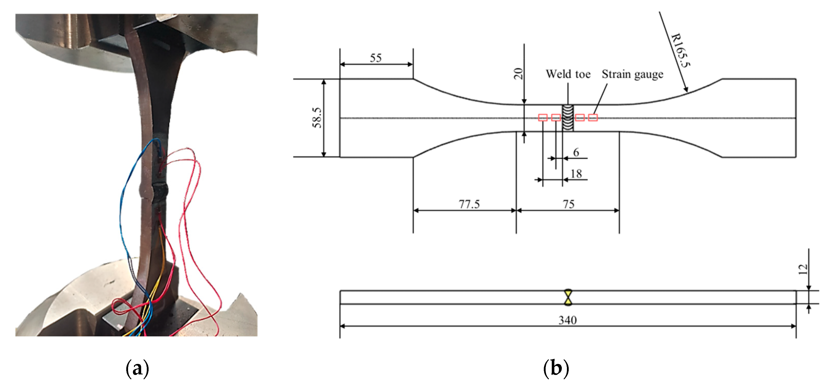
In this paper, a series of fatigue tests were conducted on butt-welded specimens using a material test system (MTS) fatigue testing machine. The material used in this test is shipbuilding high-strength 10CrNi3MoV steel. The mechanical property of material is shown in
Table 1, the chemical composition of the material is shown in
Table 2, the mechanical property of the welding wire is shown in
Table 3, the chemical composition of the welding wire is shown in
Table 4, and the welding process parameter is shown in
Table 5.
The strain and displacement data of these specimens throughout the entire fatigue failure process were recorded. By continuously training on these data, the structural response characteristics in the fatigue failure process were obtained. When conducting fatigue tests on new specimens, after the specimen starts to crack, the remaining fatigue life is predicted in real time using only the collected strain and displacement data up to the current moment. The considered welded structure are shown in
Figure 1.
However, it is not easy for a machine learning-based model to predict the remaining fatigue life of a specimen during the testing process for the following reasons:
- (1)
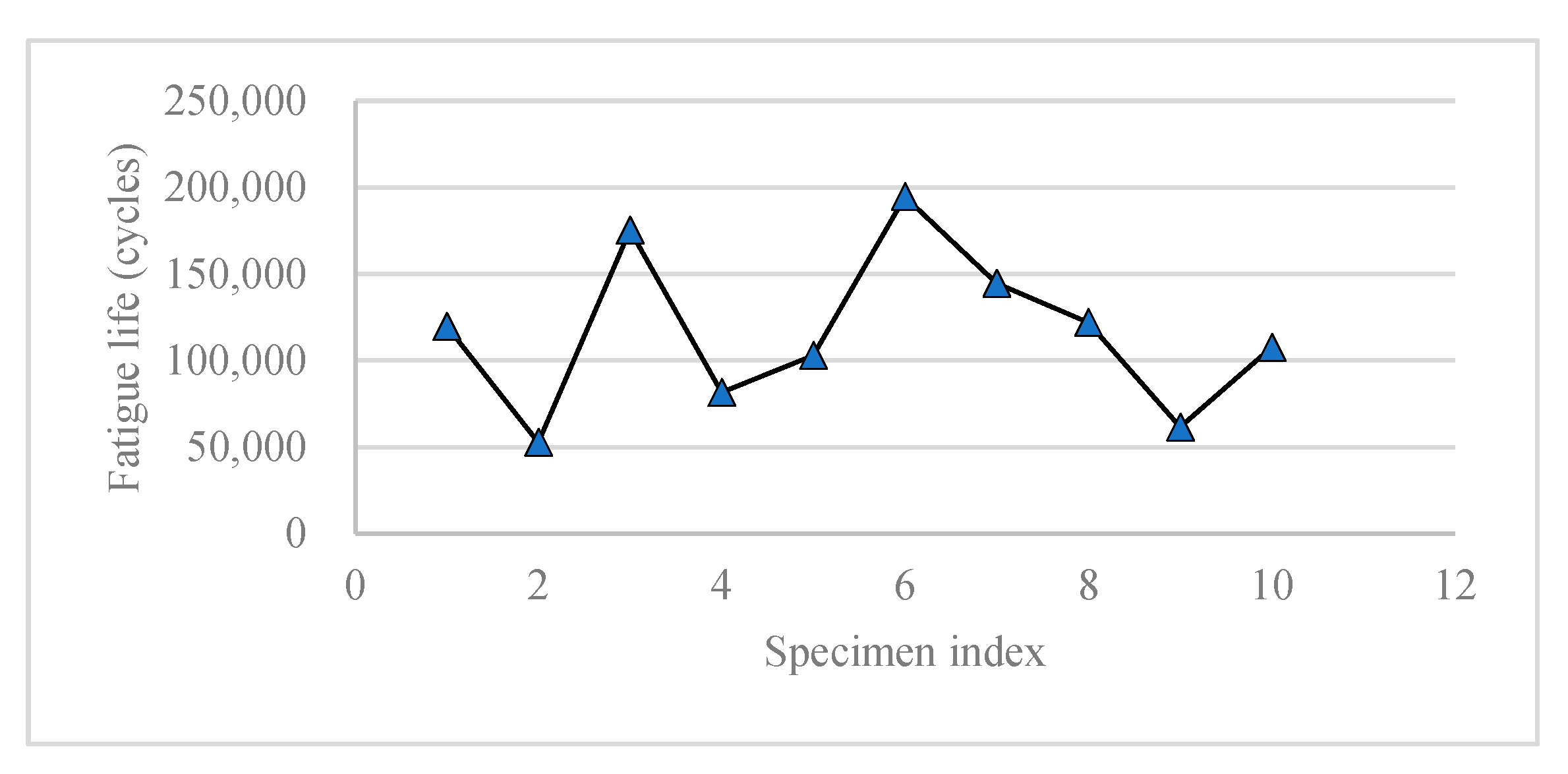
The deviation of fatigue life of different specimen even with the same welded structure is relatively large.
Figure 2 shows the numbers of cycles of fatigue life for 10 different specimens for the welded structure shown in
Figure 1b. The maximum differentiation achieves 150 k cycles;
- (2)
Different loading may be applied in the fatigue test for different specimens, which leads to different fatigue life.
For those reasons, it is hard to obtain accurate results with traditional models such as those based on Paris’ law. So, in this paper, a deep learning-based model is to be proposed for this problem.
2.2. Data Selection and Monitoring
For a machine learning-based prediction model, the selection of input data is an important factor. When welded structure starts to crack under cyclic loading in fatigue testing, it is assumed that the strains near welded joints and the longitudinal displacement of the structure can reflect such a change. Here, the signals of four strains near welded joints, longitudinal displacement of the testing structure and the cyclic loading are recorded during fatigue test.
Under the influence of sinusoidal fatigue loading, all the signals are sinusoidal, and the peak values, valley values of variables in each sampling cycle may have little changes when cracks start to propagate. However, it is found that the change of strain peak values is more obvious than the valley values during crack propagation, as shown in
Figure 3. So, only the peak values of variables (e.g., strains) are selected as the input of our prediction model. Besides, notice that the cycle number acts as a time encoding, indicating the increasing trend of a crack, and so is also adopted as an input variable in our prediction model.
Since the remaining fatigue life prediction in crack propagation and final facture stage is considered in this paper, this stage should be firstly identified. Here, let denote the peak sequence data collected up to date, and is the peak values of the collected data vector at the current moment k, and C is the number of variables in the vector. Here, C is equal to five as four strains and one displacement data are collected. The following rule is adopted to identify the crack propagation stage:
- (1)
Compute the average peak values of a variable of the previous 50N cycles and the latter N cycles, respectively, denoted as and
- (2)
If the following condition is satisfied, the moment t is identified as the beginning of crack propagation:
In the rule, N and are predetermined parameters. In this paper, we set N as 200 according to pre-experiments and = 0.05. As there are 5 variables or dimensions, once the data of a dimension satisfy the condition, the beginning point could be identified. Notably, it is hard to identify the real beginning of structure fatigue propagation. Here, the beginning point determined by the above rule just provides an implication that the data have minimal variation and the prediction can be applied. Obviously, at the current moment t, the moment before N cycles is evaluated to be the beginning or not.
2.3. Data Processing
To reduce the dimensional impacts, the collected physical data together with the cycle number in crack propagation stage are all firstly normalized to reduce the effect of different distributions of values for different dimensions and specimens. For each specimen
i, let
and
denote the original and normalized peak data vectors for current moment
k, respectively, where
t(
k) denotes the cycle number counted from the beginning of crack propagation. Then, all the data of each variable are offset by the following formula:
where
denotes the deviation vector for the original peak data. Here,
is estimated using the data in crack propagation stage for
n tested specimens as follows:
Through the above procedures, the data sequence for each specimen is normalized to dimensionless values and shifted unit to have the first value in the sequence be zero.
3. Remaining Fatigue Life Prediction Model Based on Deep Learning
Deep learning has demonstrated remarkable performance in the modeling of complex relationships [
20,
21]. Here, a hybrid approach of CNN, squeeze-and-excitation (SE) blocks, and LSTM are combined to predict RFL of considered butt-welded structures. The whole frame of the model is shown in
Figure 4. The real lines in
Figure 4 show the process of model training and the dash line shows the process of real-time prediction. In the approach, the hybrid deep learning-based model, CNN–SE–LSTM, is firstly trained to calculate a health indicator, using the data segments generated according to the data collected for trained specimens. In real-time prediction, once a sequence of data segments is obtained, the trained model is used to calculate a health indictor (HI) [
22]. With all the health indicators calculated up to date, a RFL is predicted through a particle filter-based algorithm.
In the CNN–SE–LSTM model, CNN with SE block responds to extract sequence features, while LSTM tries to predict HI values. Here, instead of using remaining fatigue life, health indicator is taken as the output of the hybrid model and is then transformed to remaining fatigue life by particle filter algorithm. By using HI, the output of the model is not an absolute value (remaining fatigue life) but a relative one (HI), which can make the approach more robust. The details of the model are described as follows:
3.1. The Input Data
In real-time prediction, once a data segment is collected, prediction models are triggered to predict the remaining fatigue life. In this paper, the input data of the prediction model are set as the current fragment of the normalized data sequence. It includes
D sequence segments and each segment includes
T cycles’ normalized information. The interval between two adjacent segments is set as
T, where
is a predetermined parameter, which could be used to control the frequency of prediction in real time. Let
x denote the normalized peak data vector for cycle
k; the relationships of the input data and the normalized data sequence are shown in
Figure 5.
As shown in
Figure 5, the peak values of
T continuous cycles form a segment. Once
D segments are formed, they are input into the prediction model to predict the remaining fatigue life. The length of the input sequence is
and the dimension is
C+1, as mentioned in
Section 2.3. The details of the model are described in the following sections.
3.2. Feature Extraction by CNN with Attention Blocks
CNN uses multiple convolution kernels in each convolutional layer to extract features from the current data sequence. In this paper, a CNN embedded with SENet [
23] attention blocks is adopted. The structure is shown in
Figure 6. In the figure, the input sequence
= (
, …,
) is firstly transformed by a 1D-SE attention block before it goes to the next layer. Each layer of CNN, such as the 1D-SE attention block, is embedded as shown in the feature.
Let L denote the layer number of the model, and denote the channel number and the output of layer l, respectively. Let denote the value in channel c at the ith position in the input data sequence, and is that of the output sequence for layer . The 1D-SE block and the convolution operation in each layer can be described as follows.
3.2.1. Channel Attention Strategy (1D-SE Block)
In each layer (l = 1, …, L), perform a reduced SE attention strategy with squeeze, excitation, and scale operators.
- (1)
Squeeze operator
: Squeeze operator averages the data in each channel c for layer l to obtain global feature
and forms the global feature vector
T. The computation is as follows.
- (2)
Excitation operator
: The importance of each channel is evaluated through two fully connected layers as
where
is the channel weight vector for layer
l,
and
are the parameters for the two fully connected layers. Here, R is the scale factor and
denotes the node number in the first fully connected layer and is set as 2 to reduce the computation. Sigmoid function is adopted for the activation function f and then the output value is limited in (0, 1).
- (3)
Scale operator
: Cumulate the weighted feature and the original input feature
for layer
l as follows:
where ⨂ denotes matrix computation point by point, and
is the transferred feature.
3.2.2. Convolution Operations
In each layer
l (
l = 1, …,
L), perform convolution
Conv(
) and activation function
sequencially. Before that,
is firstly padded to remain the same length of feature. The process could be expressed as
where
and
denote the kernel vector and output feature after convolution operations, respectively, where
K is the kernel length;
denotes a padding operator to remain the length of the feature unchangeable in convolution operations. Its padding length
d equals
, that is,
blanks are padded to one side and
blanks to the other side of the sequence. Rectified linear unit (ReLU) function is adopted as the activation function.
In the concrete implementation, set L = 3, K = 9. The channel number vector is set as (20, 20, 1). With the above process, the extracted feature Z = Y3 () is obtained.
3.3. Health Indicator Prediction with LSTM
For time series forecasting problems, LSTM model can efficiently capture the relationships between the input sequence and output sequence [
24]. In this paper, LSTM is adopted to calculate health indicators instead of RFL. Here, the following assumptions are made for HI:
- (1)
Each prediction time corresponds to a HI value.
- (2)
HI value changes linearly from 0 to 1 during the crack propagation and fracture stage.
- (3)
When HI reaches 1, it means that the remaining fatigue life is 0.
With this assumption, HI indicators imply the variation trend of fatigue remaining time. For a certain specimen, at each prediction cycle number k, the reference HI value is calculated as , where CPL is the real fatigue life in crack propagation stage. By using HI, the output is uniformly mapped to the interval of [0, 1], and so the predicted model can greatly reduce the output difference for different specimens with different fatigue life. This may facilitate model convergence during training.
The model structure of LSTM adopted here is shown in
Figure 7. The features extracted by CNN are reshaped into feature sequences through a fully connected layer first. Then, a two-layer LSTM followed by a fully connected layer is used to calculate health indicators.
3.3.1. Feature Reshaping
Fold the obtained CNN feature
to
feature sequences, denoted as
where
, which are input into a full-connection layer to further extend the features.
where
is the weight vector and the activation function
f is sigmoid function, and
is the output feature and
is the output feature’s length. In our setting,
= 16.
3.3.2. LSTM Model
A two-layer LSTM model followed by a fully linear connected layer is used to calculate a health indicator sequence, which is expressed as
where
is the predicted output HI sequence, the predicted HI value (
) for the current data sequence is set as the last element in the
list, which is denoted as
. Notice that at each prediction time (cycle)
k, the reference HI value is set as
.
3.4. The Loss Function of the Model
The loss function of the model directly calculates the mean square error between the calculated health indicator
and the reference health indicator
,
where
,
and
are the current cycle number and the real crack propagation life for specimen
i, respectively.
3.5. Transformation of Health Indicator to Remaining Fatigue Life
As mentioned before, HI values imply the variation trend of RFL and linearly vary with it, so all the predicted HI values in history form a HI sequence and can be fitted into a function. The predicted remaining fatigue life is defined as where the function value equals 1. In the selection process of fitting function models, it is necessary to use function model that can describe most of the HI curves. We have used other functions such as linear function, quadratic function, exponential function, etc. in the selection process. Cubic functions have better fitting performance for HI curves compared to the above functions. The cubic function has a good balance between the number of parameters to be estimated and the fitting performance. Here, a cubic function is adopted to describe the variation trend of HI values. Moreover, particle filtering (PF) algorithm is adopted to optimize the fitting function. More information about PF can be found in the literature [
18].
Express the adopted cubic function as , where denotes HI variable, k is the sampling cycles counted from the beginning of crack propagation and fracture stage, and a, b, c, d are four parameters, which are updated iteratively. The transformation process is as follows:
- (1)
Initialize a, b, c, d according to pre-experiments, denoted as a[0], b[0], c[0], and d[0], and set initial iteration number h = 1.
- (2)
Apply PF algorithm to update the four parameters as a[h], b[h], c[h], and d[h] once a new HI value HTh for the current prediction cycle is obtained, i.e., the predicted HI sequence is updated.
- (3)
Compute the sampling cycles when HI arrives at the failure threshold 1 according to the current cubic function.
- (4)
Set h = h + 1 and return to Step 2 if a new HI value is predicted, or else terminate the process.
Note that a[0], b[0], c[0], and d[0] are predetermined with pre-experiments. To obtain better results, two sets of initial function parameters are adopted, one for increasing trend and the other for decreasing trend of strain data. In real-time prediction, by detecting the varying trend of strain data, different initial parameter set is selected.
4. Results and Discussion
The proposed model is conducted on a computer platform with Windows 10 operating system, AMD Ryzen 5 3600 CPU, GeForce RTX 1660Ti graphics card, 6 GB graphics memory, and 16 GB system memory. The software programs are all built on Python 3.9.12, which mainly uses three third-party libraries: numpy, pytorch, and scipy.
4.1. Model Training Setting
In our experiments, fatigue testing is executed on 28 different specimens of butt-welded structures. The datasets for 13 specimens numbered from Spe. 1~13 are selected randomly as training sets and a total of 7739 data sequences are generated according to the data. The data for the other 15 specimens numbered from Spe. 14~28 are used as test data. Notice that the specimens of Spe. 1~24 are applied with a frequency of 8 Hz, a stress ratio R of −1, and a stress level of 0.45 with a peak loading with 54 kN, while the specimens of Spe. 25~28 are applied with varying peak loadings.
To decrease the effect of the order settings of strains and improve the model robustness, the strain signal channels are randomly disrupted during model training. The following parameters are set as follows in training:
- (1)
Adam strategy is adopted to optimize model parameters;
- (2)
Learning rate is set as 0.0005;
- (3)
Drop out parameter is set as 0.3;
- (4)
Batch size is set as 32;
- (5)
Training epoch is set as 200.
These parameters related to model training are determined by pre-experiments, which can make the training process converge to stable and not overfitting.
4.2. Model Performance Metrics
To evaluate the model performance, the mean scatter defined in Formula (11) and the mean relative deviation defined in Formula (12) are used to measure the prediction [
25].
where
and
are the predicted and the real remaining fatigue life, respectively, at the
ith time segmentation, and
denotes the considered prediction time span.
Obviously, MS evaluates the robustness of prediction results while evaluates the prediction precision. In the following experiments, the prediction is independently executed three times for each specimen and the average MS and are computed to evaluate a model.
4.3. Strategy Validation Analysis
To verify the contribution of each module, four versions of models are tested, that is, CNN, LSTM, CNN–LSTM, and CNN–SE–LSTM (i.e., the proposed model). The performance of the four models is compared in different crack propagation stages and for different specimens, respectively.
Table 6 shows the average
and MS of the test data for specimens Spe. 14–24 in different crack propagation stages. The crack propagation stage is divided into four sub-stages, S
≤25%, S
25%~50%, S
50%~75%, and S
75%~100%, where the subscript denotes the ratio of the current cycle number to the whole crack propagation life.
From the
Table 6, it can be seen that the CNN–SE–LSTM model shows the best performance in terms of
and MS scores. It indicates that CNN, LSTM, and SE module have their own contributions to the final model. That is, the CNN model captures the local invariance characteristics of the sequence, while LSTM helps to extract the features between the front and back segments in a sequence. Through SE module, the channels with obvious changes are given large weights, which helps the model to extract salient features of the whole long sequence.
Figure 8 visualizes the SE blocks’ function for a test specimen.
Figure 8a shows the four-channel strain peak curves and
Figure 8b shows the weights for different channels at the prediction time τ, Strain 1 has the earliest change trend and has the most obvious value on the attention weight. Obviously, it can be seen that SE blocks helps the model capture large changes in channels.
Table 7 and
Table 8 shows the average
and MS scores of the four versions of models for different specimens numbered from Spe. 14–24, respectively. It can be seen that the CNN–SE–LSTM model obtain better results than other two models in terms of
and MS scores on average. The CNN–SE–LSTM model can maintain optimal or suboptimal performance, especially in terms of MS scores.
4.4. Result Analysis for the Specimens under the Same Loads
To further verify the proposed real-time prediction method, the evaluation metrics at different sub-stages for the tested specimens numbed from 14 to 24 are listed in
Table 9. All the specimens have the same loadings with those for training.
From
Table 9, the following observations can be obtained:
- (1)
The strain gauges’ positions have effects on prediction performance. For Spe. 14–15, 22–24, the scores are relatively larger than those for Spe. 16–20. After checking the cracks of these specimens, it is found that the crack happens on the same side of the attached strain gauges for Spe. 14–15, 22–24. The reason for this is that strain gauges on the same side of the crack are more sensitive to changes in strain, resulting in earlier predictions of remaining fatigue life for these specimens. It is well known that the prediction in early stages is more difficult due to slight changes in collected data. Therefore, the average scores are relative larger for those specimens than others.
- (2)
The model obtains relative robust prediction for all the tested specimens. As shown in
Table 9, the average MS score is less than 1.5, which means that the ratio of the prediction results and the real remaining fatigue life is less than 1.5. Notice that the remaining fatigue life trend to 0, and the ratio of 1.5 indicates a very good performance.
- (3)
In the S≤50% stage, the model showed a high error, which was mainly caused by two factors. First, the prediction results in the early stage were mainly affected by the initial values of the parameters set in the PF algorithm, which resulted in a large deviation in the S≤50% stage. The selection of the initial values of the parameters was equivalent to the intervention of prior knowledge on the prediction of the early results, which always had a profound impact on the early prediction. Second, the HI curve did not change in a fixed way. The PF algorithm needed to update the parameters of the cubic function according to the changes of the HI curve. Therefore, when it reached the later stage, the model showed a better performance in accuracy, because the PF algorithm obtained enough information of the HI curve.
Figure 9 illustrates the predicted and real remaining fatigue life curves varying with cycles for specimens Spe. 14–17. It indicated that the differences between the two curves reduce gradually, and the proposed model can continuously correct HI functions according to the predicted HI values in history in the prediction process.
4.5. Result Analysis for the Specimens under Different Cyclic Loadings
In order to investigate the generalization performance of the proposed model, the model is also used to predict the remaining fatigue life for specimens under different cyclic loadings. However, different from the original proposed approach, the initial parameters of cubic function for health indicators are provided by least square method as the variation trend of health indicators may be greatly different from those for the specimens under the same cyclic loading in training. By using the least square method, a linear function is generated to fit the first 20 health indicator values and the yielded parameters are set as c[0] and d[0], while the other two parameters a[0] and b[0] are set as zero.
Table 10 provides the experimental results of the CNN–SE–LSTM approach for four specimens with different cyclic loading conditions during testing, i.e., Spe. 25–28.
Figure 10 shows the visualized prediction results. The experimental results show that the proposed model is capable of producing reasonable predictions for the remaining fatigue life. Even in the last sub-stage, the ratio of the predicted and the real remaining fatigue life is less than 2.0. This capability arises from (1) the normalization of the data sequence, which can reduce the impact of differences in peaks of various physical quantities; (2) the indirect prediction of the remaining fatigue life through health indicator, which positively enhances the generalizability of the prediction methodology.
However, it can be seen from
Table 10 and
Figure 10. that the results for specimen Spe. 28 are inferior to those for other specimens. This can be explained by the fact that prediction accuracy is greatly affected by the function of calculated health indicators. As analyzed in
Section 4.4, the selection of the initial values of the parameters has a critical impact on the accuracy of the early prediction. When the load information is unknown, the ©nitial values of the parameters cannot be directly specified. In this paper, the least squares method is used to estimate the initial values, which makes it easier for the prediction deviation to be too large in the early stage. Secondly, when the actual health indicator curve does not follow a linear pattern, the predictive performance of the model in the early stages will further deteriorate.
As for the running time, the experimental results are shown in
Table 11. the maximum and the average running time is 59.3 ms and 37.3 ms for the tested 15 specimens, respectively. That is, the prediction results can be updated every 60 ms, which can satisfy most real-time application requirements.

 ,
, 


