Article

Radar-Based Particle Localization in Densely Packed Granular Assemblies

1
Institute of Microwave Systems (HFS), Ruhr University Bochum, Universitätsstraße 150, 44801 Bochum, Germany
2
Institute of Energy Plant Technology (LEAT), Ruhr University Bochum, Universitätsstraße 150, 44801 Bochum, Germany
*
Author to whom correspondence should be addressed.
Processes 2023, 11(11), 3183; https://doi.org/10.3390/pr11113183
Submission received: 11 October 2023 / Revised: 26 October 2023 / Accepted: 2 November 2023 / Published: 8 November 2023
(This article belongs to the Section Particle Processes)

Abstract

:
Particle tracking in densely packed granular assemblies is of great interest in mechanical process engineering. In this contribution, a radar-based system for particle localization as an initial step towards tracking is presented. This system comprises six transmitting and receiving antennas forming a “multiple-input multiple-output” setup positioned around a cuboidal reactor. The reactor is a standard batch grate system, which contains stationary spherical polyoxymethylene particles with a 10 mm diameter and a spherical steel tracer particle with a 20 mm diameter. The tracer is positioned at various locations at an optically transparent reactor wall. Electromagnetic waves must pass through the remaining three reactor walls to detect the tracer particle. Operating in the Frequency Modulated Continuous Wave mode within a 1.5 to 8.5 GHz frequency range, we compared radar-detected tracer positions with those from camera images. The results demonstrate a vertical localization accuracy with a standard deviation of σ v e r t = 0.86 cm and a horizontal position accuracy with σ h o r = 0.17 cm. This study not only presents the achievements of radar-based particle localization but also delves into the potential and challenges of applying this technology to a specific measurement scenario within mechanical process engineering.

1. Introduction

Moving granular assemblies occur in many applications in process industries. Examples are fluidized beds (e.g., granulation) [1], moving beds (e.g., lime shaft kilns) [2], grate type systems [3] (e.g., combustion of wood chips), or rotary kilns [4] (e.g., cement production). For the correct processing of the particles, their movement pattern is an important piece of information to ensure sufficient residence time in a reactor or to assess particle mixing and segregation in the granular assembly. However, as the particles are typically opaque, optical methods are usually not suitable to obtain information from the inside.
A couple of non-optical methods have been established in the past, which can provide this information, with each having its specific advantages and disadvantages. A thorough overview on these techniques is given by Amon et al. [5].
Tomography in different wavelengths (X-ray [6], microwave [7], millimeter-wave [8], CT [9]), and magnetic resonance imaging (MRI) [10] offer the potential to visualize each individual particle in a volume. Temporal resolution is usually limited and the respective setups are costly and not available in sizes applicable for industrial systems. An alternative approach is to track single or a limited number of tracer particles at high sampling rates. Based on an analysis of the statistics of the movement of the tracer particle, the system dynamics can be assessed. Technologies based on this principle are positron emission particle tracking (PEPT) [11], radioactive particle tracking (RPT) [12], magnetic particle tracking (MPT) [13], and the method addressed in this study: radar-based particle tracking. PEPT and RPT rely on tracers doped with radioactive isotopes, emitting radiation that can pose safety concerns and rendering them unsuitable for many industrial applications. MPT does not share this disadvantage, instead, it allows for the measurement of particle orientation in parallel to particle location. However, the magnetic field strength generated by the tracer particle decays rapidly with the distance to the tracer particle, which limits the size of the reactor geometries that can be examined. Additionally, the density of magnetic materials is high, which can make it difficult to design appropriate tracer particles for a system of particles with lower density.
This work focuses on tracking particles using high-frequency electromagnetic waves. This approach offers several advantages, including the use of electromagnetic waves with wavelengths suitable for penetrating various dielectric materials, like limestone or magnesite, which are common in industrial applications. Moreover, the selected wavelength falls within the centimeter range, ensuring safety when dealing with organic substances.
In contrast to tomography, our imaging approach does not rely on evaluating the attenuation of electromagnetic waves, instead, it focuses on the analysis of the reflection of individual waves. In this process, electromagnetic waves are emitted, reflected by objects, and then measured by receivers. To achieve three-dimensional localization, we employ multiple transmitting and receiving antennas, forming a “multiple-input multiple-output” (MIMO) system. The resolution of the measurement system greatly depends on the number of transceivers and receivers [14,15]. Therefore, achieving high resolution requires a significant number of these components; however, the same holds true for tomographic image reconstruction as demonstrated in [16] for a 2D arrangement. Here, a 10 × 10 cm area was surveyed using 16 transceivers and 15 receivers and a tomographic image reconstruction. Expanding to a three-dimensional measurement setup is possible but incurs substantial additional hardware costs. Traditionally, tomography addresses these challenges through scanning processes, involving movement of either the measurement object [17] or the measurement system [18]. However, this approach results in longer measurement times, making it less suitable for real-time applications that require imaging moving processes.
Therefore, our goal is to develop a MIMO system capable of capturing a three-dimensional volume without relying on excessively complex hardware. In this study, we have employed a radar-based imaging approach. In contrast to conventional tomography, our methodology involves tracking the reflections originating from the objects under observation. Utilizing reflection compensation techniques, we can reconstruct the path of the radiation, thereby generating an image of the measurement area. While high sampling rates are essential for accurate representation of all particles in the bulk material, we recognize the challenges of extensive sampling and shift our focus to tracking a single electromagnetic tracer, similar to PEPT, RPT, or MPT. This tracer stands out from the background, enabling effective tracking even in scenarios with significant undersampling.
Radar object tracking is, in principle, well established. For example, human target tracking in buildings [19] or tracking of vehicles using automotive radar [20,21]. An overview of radar object tracking is given by [22].
Still, the present approach differs from known radar object tracking in several ways:
  • It deals with tracking markers within bulk materials, where assumptions of free space or homogeneous backgrounds no longer apply due to refraction effects, scattering, and varying propagation velocities.
  • Wave propagation occurs within particles that are no longer assumed to be small compared to the wavelength, leading to potential imaging artefacts and particle localization challenges. Other comparable works in [23,24,25] use frequencies in the range from 8.2 GHz up to 12.4 GHz but at the same time assume a homogeneous background medium such as sand [23,24] or mortar [25]; both media are significantly finer-grained than the medium used in this work.
  • Industrial reactors are typically large, requiring a considerable number of antennas to ensure interference-free imaging. Our work operates in an undersampled three- dimensional region, presenting additional localization challenges. These aspects ensure the novelty of the present contribution.
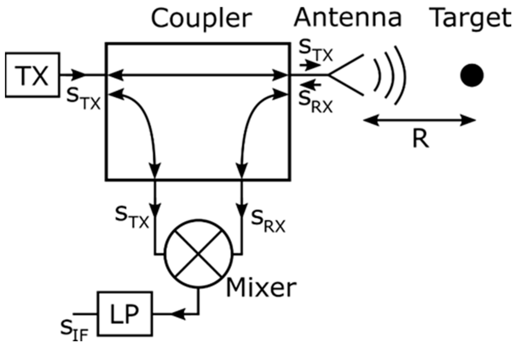
In this study, we present a MIMO system based on the Frequency Modulated Continuous Wave (FMCW) radar approach. This system employs six antennas operating in the 1.5 GHz to 8.5 GHz frequency range, ensuring accuracy, calibration capability, and flexibility by utilizing a vector network analyzer (VNA).
Our test setup involved a laboratory-scale cuboidal batch grate system filled with resting spherical polyoxymethylene (POM) particles and a steel tracer particle. The antennas were positioned so that electromagnetic waves penetrated the bulk to detect the tracer particle. We compared different particle positions detected by the radar system with camera images of the visible tracer particle to validate the accuracy of the radar-based localization system across the entire granular material volume.
The novelty of this work lies in its application of radar-based imaging to track and localize individual tracer particles within complex industrial systems, addressing challenges specific to these environments. We can accurately detect tracer particle locations in the grate system, focusing initially on resting particles. The use of high-frequency electromagnetic waves enables successful tracking within industrial reactors.
The article’s structure is as follows: Section 2 reviews radar principles and imaging, Section 3 presents the measurement setup, Section 4 discusses measurement results, and Section 5 concludes the article.

2. Radar Technology

Please note that we deliberately have written the introduction to the radar technology in a basic form to account for the readership of Processes who might not be experts in radar applications. Radar, short for radio detection and ranging, is a technology that utilizes electromagnetic waves to detect and locate objects in its surrounding environment. While radar was initially developed for the purpose of locating ships and aircraft, it is now extensively used in industrial measurement technology as well. In this context, we will focus solely on primary radar (passive tracer), disregarding secondary radar (active, responding tracer). Primary radar can be further categorized into pulse radar and FMCW radar.
Pulse radar operates by emitting a short electromagnetic pulse, which can be either in the baseband or modulated onto a carrier signal within a specific frequency range. The distance to the radar target is obtained by measuring the pulse transit time, while the directional information is determined through the angular position of a well-focused antenna. On the other hand, FMCW radar works by transmitting an electromagnetic wave with a continuously changing frequency. In this work, we apply an FMCW radar approach, since the bandwidth of pulse radar systems is typically limited by the finite pulse width, while FMCW systems allow for the transmission of broadband signals by sweeping the frequency of an oscillator. As will be shown later, the minimum distance at which two objects can be distinguished, unambiguously scales with the bandwidth of the system, which emphasises the great advantage of FMCW sensors. In the following section, we will give a short introduction to the structure of an FMCW radar and the according signal processing.

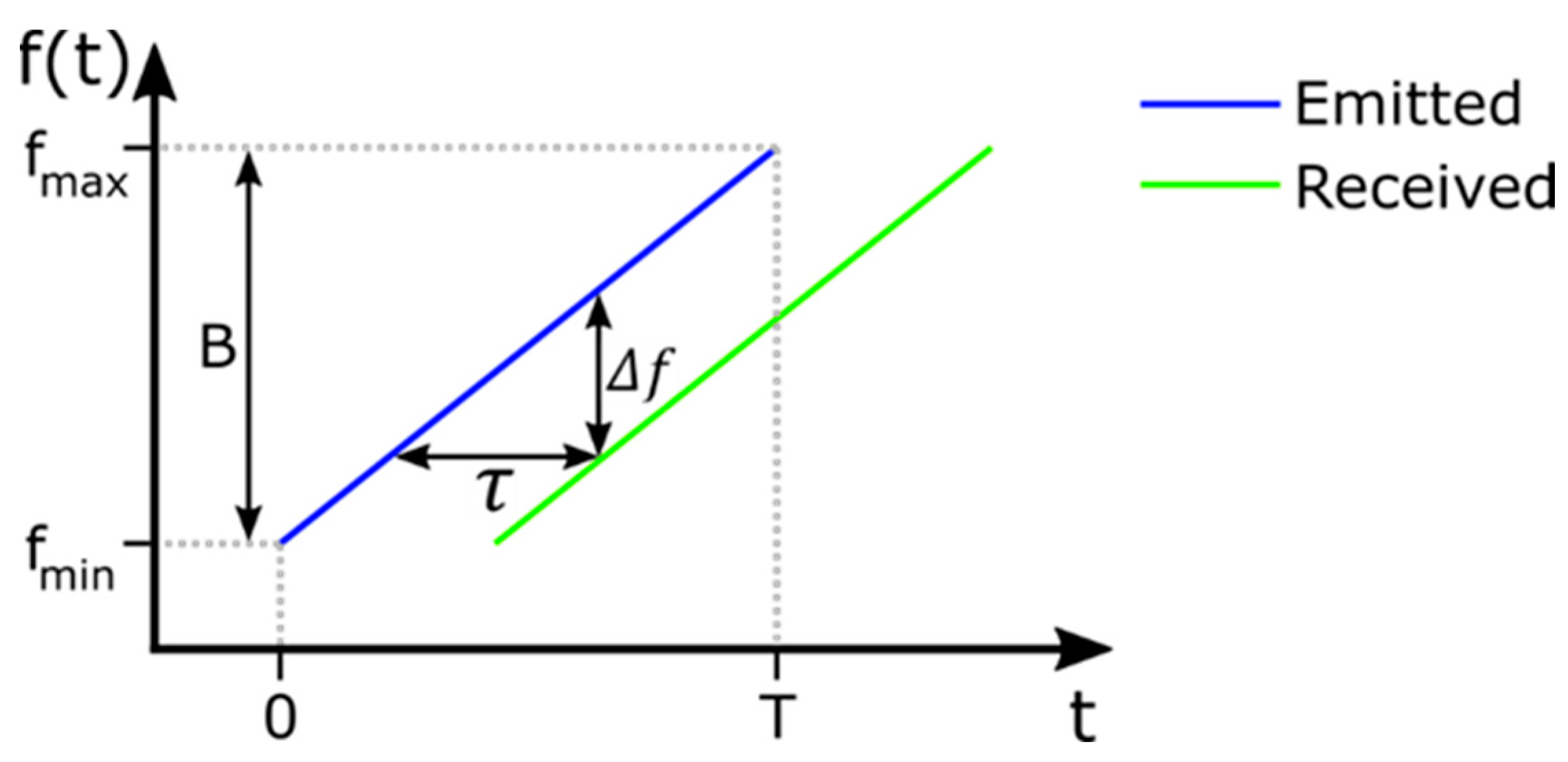
2.1. The FMCW Method
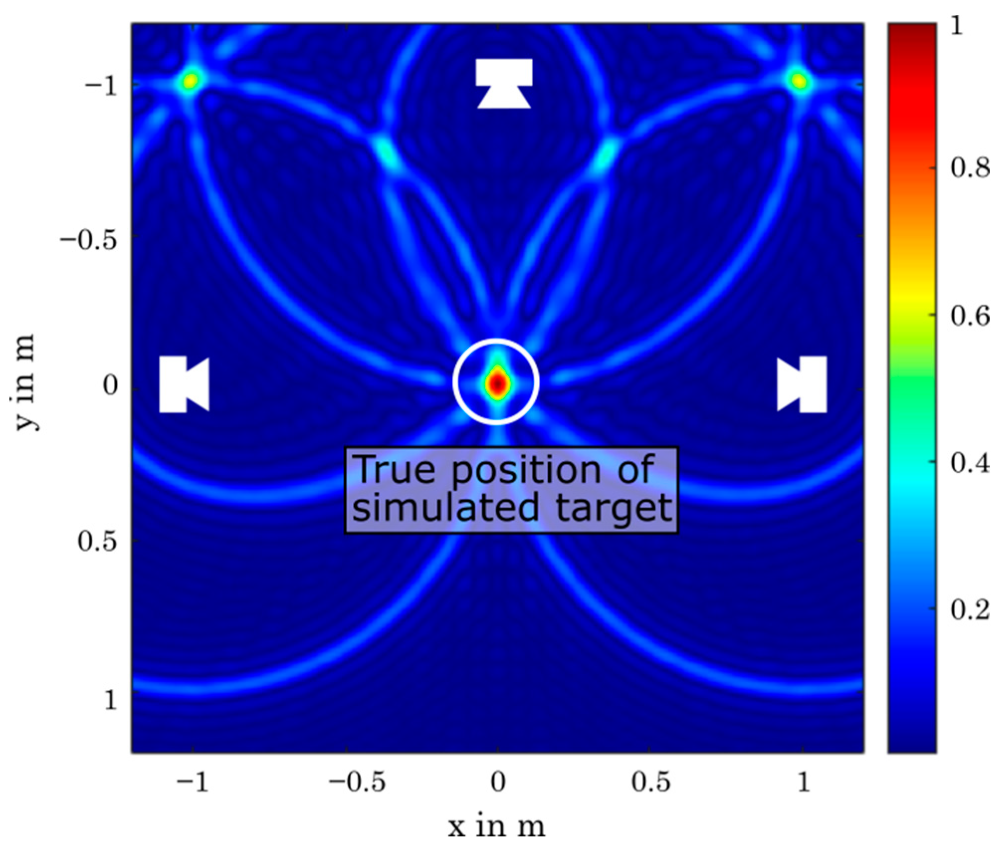
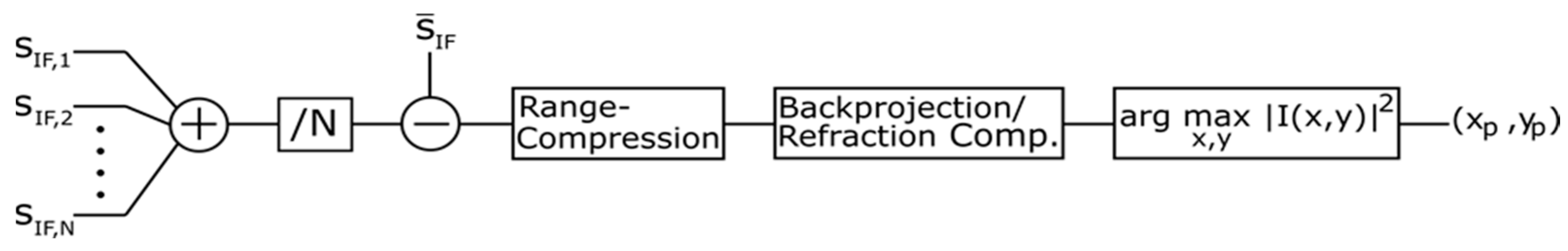
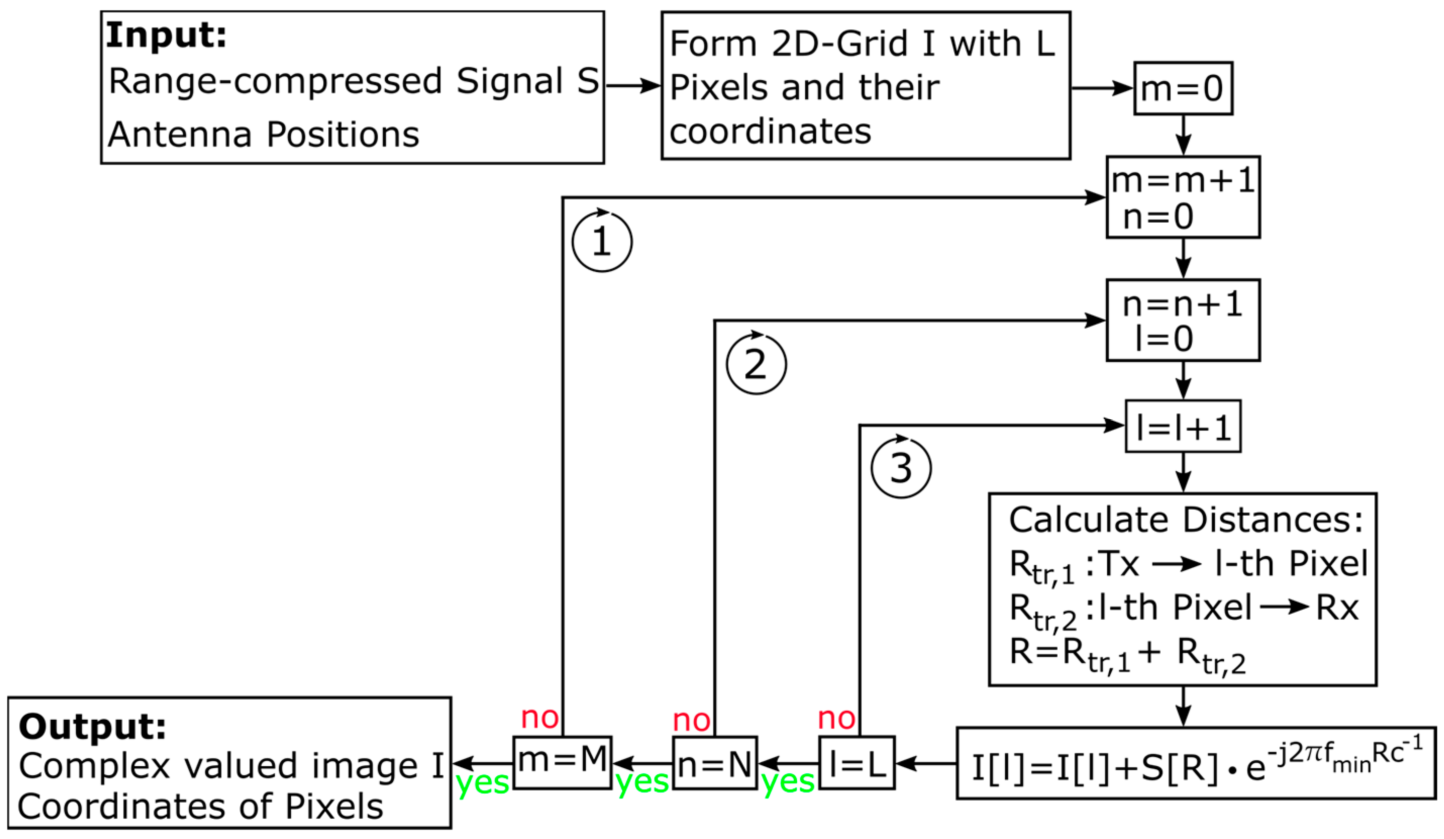
Figure 1 shows a simplified configuration of an FMCW system with the respective analogue signal processing. Here, the transmitter T x generates a transmission signal s T x t , which is divided into two paths by a coupler. One part of the signal is emitted towards the target through an antenna, while the other part is directed to a frequency mixer.
When the transmitted wave encounters a target, a part of it is reflected and transmits back to the antenna, where it is received, leading to a signal s R x t . This received signal is also directed to the mixer by the coupler where the signal s R x t is multiplied with the transmission signal s T x t .
The resulting mixed (multiplied) signal is subsequently low-pass filtered (LP). This is necessary because the output signal must be available in digital form for further signal processing and the analogue–digital converter have a limited sampling frequency. Note that the high-frequency part of the signal is not needed for the evaluation of object location, as will be shown later. In the further proceedings, we refer to the filtered output signal as the intermediate frequency (IF-)signal s I F ( t ) . For an efficient signal processing, it is necessary to find a mathematical description of this signal. After some mathematical treatment as described in Appendix A, s I F ( t ) can be given as:
s I F t = cos 2 π Δ f t + ϕ τ , t 0 , T ,
This shows that the IF-signal contains an additional phase shift ϕ depending on the round-trip time τ , which can be ignored for now but is of central importance in the radar imaging process. The round-trip time τ , which is a direct measure for the object distance R, as τ = 2 R c 0 , can be found by analyzing the frequency Δ f of the signal s I F t . This can be achieved by applying the Fourier transform to s I F t and substitute:
τ = Δ f B T ,
with B being the bandwidth of the system, calculated as the difference between the minimum and maximum frequency of the emitted signal.
This step is often referred to as range compression. For a more detailed discussion of the signal processing and the related mathematically relationships we refer to [26]. In Appendix B we briefly discuss the conditions needed to track multiple tracer particles.

2.2. Radar Imaging

After applying range compression on the IF-signal, the received data is in the range domain, providing information on the distance of a target. However, these results are only one-dimensional as they only state that the target can be found in a certain distance but the angle is not clearly defined. Recalling Figure 1, a target at distance R can be found anywhere on a sphere with a radius corresponding to R . To obtain additional information, one can use a moving well-focused antenna, so that the target is only visible in one direction. However, this procedure is only applicable if the movement of the target is neglegible during the time of antenna movement, which is typically not the case for the given application. Another well-studied approach is to use multiple antennas, where each antenna can serve as a transmitter and a receiver. Here, one antenna emits an electromagnetic wave, while all other antennas act as receivers. By switching the emitting antenna, it is possible to obtain information about the exact location of the target in the measurement environment. Figure 2 shows the arrangement for two antennas and a metallic sphere.
The solid lines show all possible target positions for a given reflection and transmission measurement, the dashed lines denote the distances R P , T x for the reflection measurement between the particle and the transmitter, and R P , R x is the distance between the particle and the receiver. Furthermore, R t r , 1 and R t r , 2 are two distances which will be used in signal processing to evaluate the transmission measurement.
For the reflection measurement, the transmitter T x on the left side emits an electromagnetic wave that is reflected by the particle and received again by the transmitter itself. Using the results for range compression from the previous section, one can determine the target distance R P , T x between the transmitter and the particle. Also, the overall distance traveled by the wave is 2 R P , T x since the radiation and reception of the wave takes place at the exact same place, whereby the round-trip time is found by τ = 2 R P , T x c 0 . However, the only statement that can be made is that the target is on a circular path at distance R P , T x from the transmitter, as shown in Figure 2, as there are multiple positions that lead to the same IF-signal. Therefore, a separate receiver R x at a different point in space is used but, according to Figure 1, the received signal s R x t is still mixed with the transmitting signal from T x . Therefore, range information can still be achieved with the procedure from the previous section, and we refer to this measurement as the transmission measurement. However, in contrast to the reflection measurement, the distance between the transmitter and the particle and the receiver and the particle is not necessarily the same in this configuration. The total distance travelled by the wave is made up of the distance between the particle and the transmitter R P , T x and the distance between the particle and the receiver R P , R x . If the measured total distance is R t r = R P , T x + R P , R x , the particle is located somewhere on a curve, so that the distance R t r , 1 from the transmitter to the curve and R t r , 2 from the curve to the receiver fulfils R t r = R t r , 1 + R t r , 2 . Therefore, the particle can be found on an ellipsoid with the transmitter and receiver in the focal points. In reference to Figure 2, it shows that the circle and ellipse drawn from a pair of transmitters and receivers meet at a certain point in space. This intersection point corresponds, in the case of a solid metal sphere, to the front of the sphere since electromagnetic waves cannot penetrate the particle.
To form an image, a straightforward solution is to superimpose the range-compressed signals for each pair of antennas. This procedure is commonly referred to as the backprojection algorithm. Here, a grid of pixels is generated, where each pixel is assigned a coordinate in space. Assuming the antenna position is also known, one can calculate the distance between antenna and pixel and find the value in the range-compressed signal. This can be performed for the reflection as well as for the transmission measurements. Adding the corresponding range-domain values at all pixels leads to an image of the measurement environment. However, the range-compressed signals are complex valued, meaning that each sample in the signal contains an amplitude and a phase information as was already described in the previous section. From theory, it can be shown that a target in free space leads to a phase shift of ϕ τ = 2 π f m i n R 1 + R 2 c 0 , where R 1 and R 2 denote the distance from the particle to the transmitter ( R P , T x in Figure 2) and receiver ( R P , R x in Figure 2), respectively. Therefore, one must compensate for the phase shift to achieve a constructive superposition of the range-domain signals at the point of the target. The details of the procedure of the backprojection algorithm can be found in Appendix C.
To illustrate the result of the presented imaging method, we simulated an ideal point scatterer in the center of a circular aperture, using frequencies in the range from 1.5 GHz to 8.5 GHz according to the measurement system. The result of the imaging is shown in Figure 3. The image also shows the position of the particle as well as the positions of the antennas depicted in white. For the simulation, the point scatterer was placed in the center, while the three antennas were placed on a circle with a radius of 1 m in relation to the particle. Since the coordinates of the antenna positions as well as the position of the particle are known beforehand, the distance and the round-trip time can be calculated by assuming that the wave propagates at the speed of light.
After the round-trip time and the frequency of the emitted chirp signal are found, both can be inserted into the formula for the IF-signal in (1). Thus, the raw data for the given constellation can be calculated analytically. Feeding the raw data into the backprojection algorithm presented in Section 2.2 finally leads to a reconstruction of the point scatterer.
Figure 3 contains the absolute values for each pixel and the image was normalized on the maximum value. This ensures that the maximum value is one as can be seen from the color bar. It clearly shows that the circles and ellipses created by the backprojection algorithm meet exactly at the point of the simulated target in the center. However, it can be seen that other targets seem to form in the upper left and right corners of the image. These targets are artifacts caused by the small number of antennas and can be avoided by evaluating the signal processing for additional antennas.

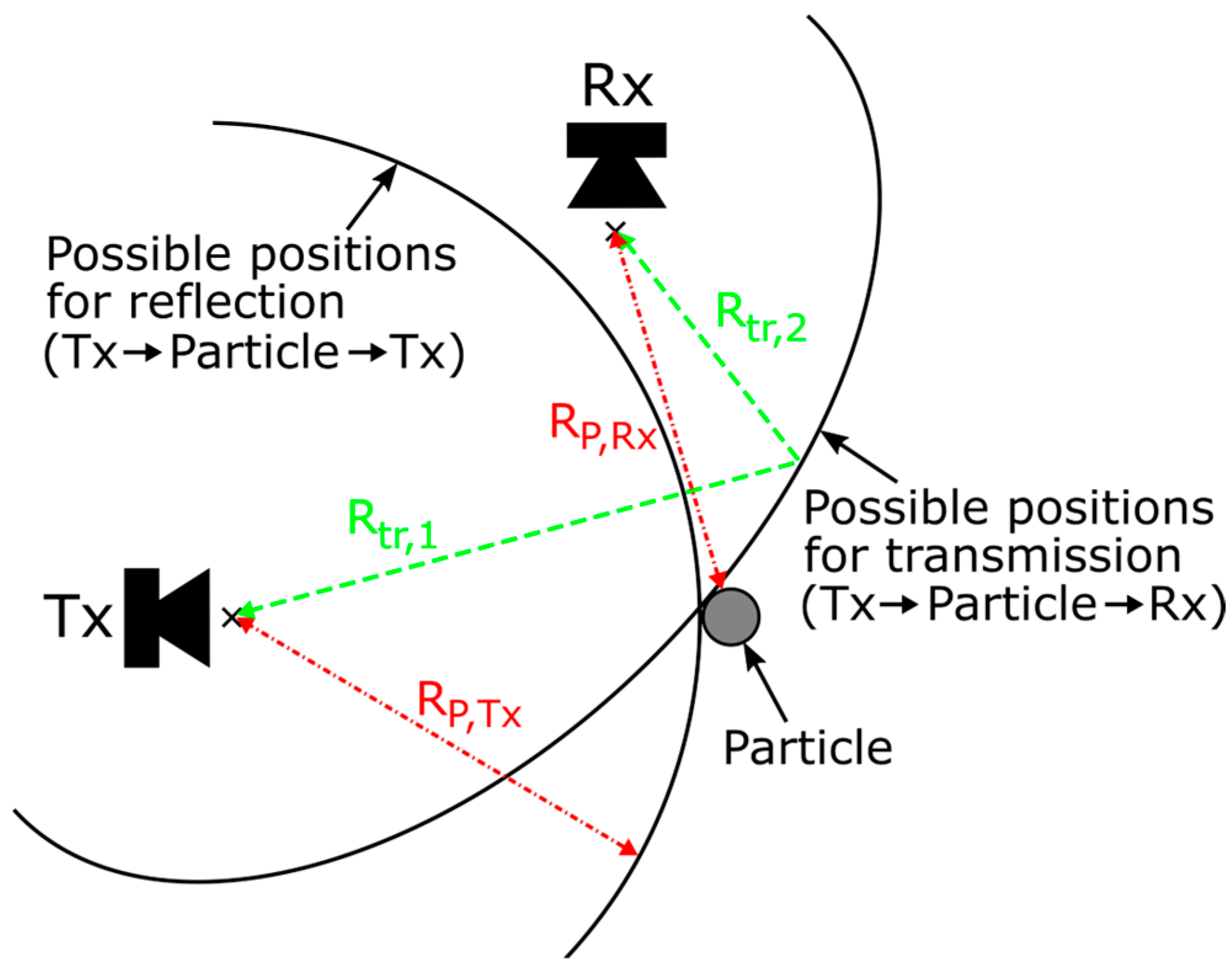
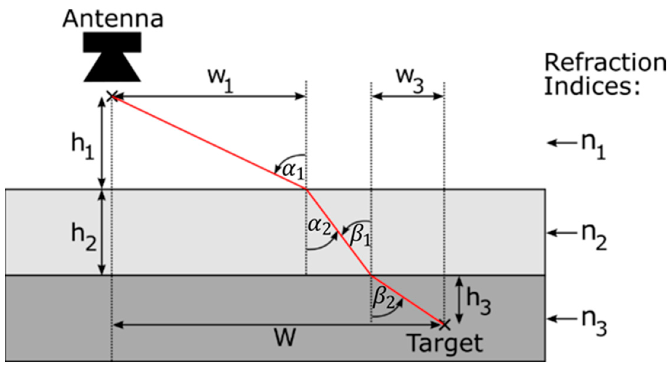
2.3. Refraction Compensation
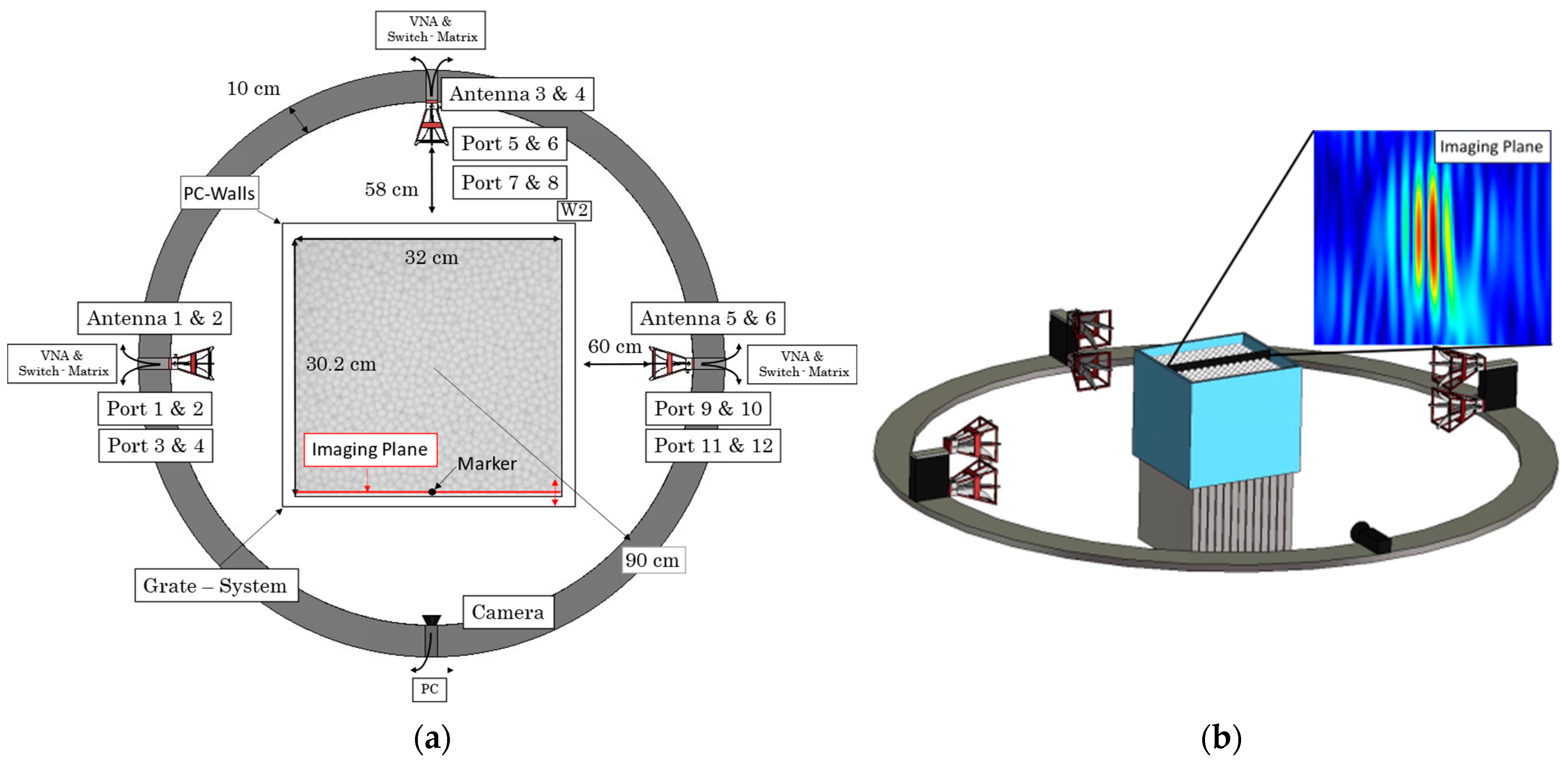
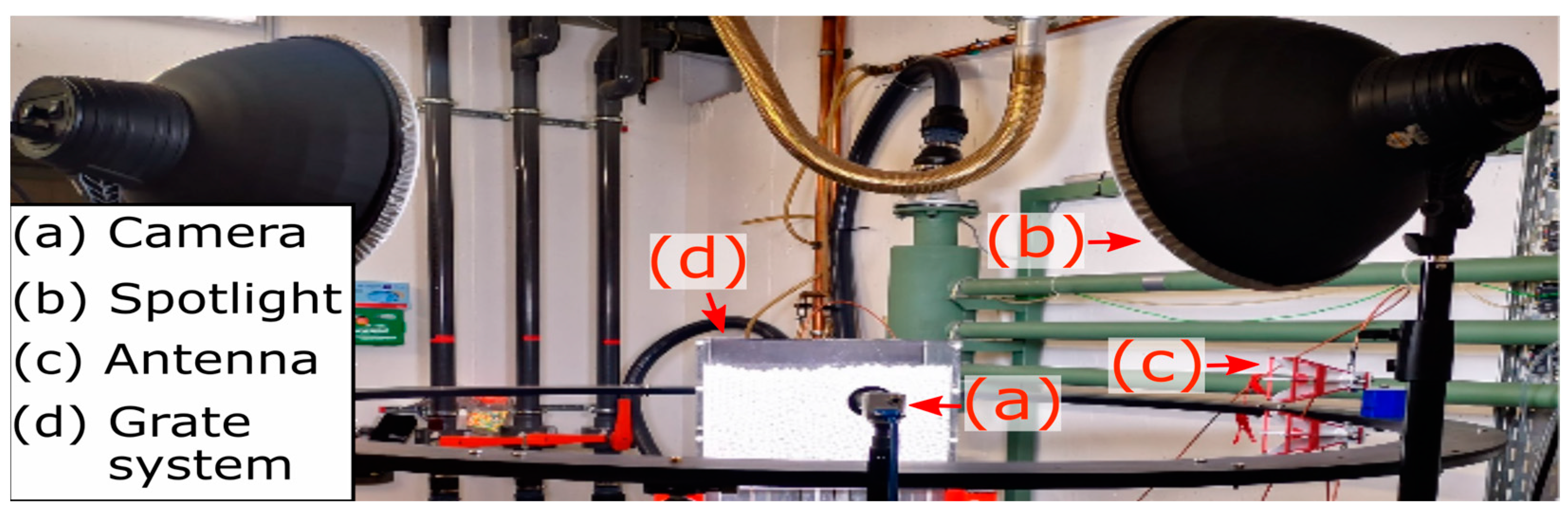
All previous discussions have been based on the assumption that the wave propagates in a homogeneous medium. However, for the given application wave propagation will occur in multiple media with varying electromagnetic behaviours. In this section, we will give an introduction into the effects occurring at material boundaries. Regarding Figure 4, the dielectric interface can be approximated as flat and the antenna is located in a vertical distance of h 1 in reference to the surface. The first layer has a thickness of h 2 , while the target is located in the second layer at a distance of h 3 . The overall horizontal distance between antenna and target is denoted by W .
As long as the curvature of the surface is large in comparison to the wavelength, the wave propagation can be described by a ray approximation as shown by the red line. For this scenario, two effects can be identified. First, the velocity of the wave varies depending on the material parameters. If the wave propagates in free space, the velocity of the wave is the speed of light c 0 . Inside a material, however, the velocity depends on the relative permittivity ε r and permeability μ r of the material. The permittivity ε r describes the polarization behaviour of the material in the presence of an electromagnetic field, while the permeability considers any magnetic properties. As most materials used for radar applications are not magnetic, we will neglect the permeability and define the refraction index as n = ε r . Using the refraction index, the velocity inside a material can be calculated as c = c 0 n . Therefore, if the refraction indices n 1 to n 3 for the three layers as well as the path of the wave between antenna and target are known in Figure 4, the round-trip time τ can be calculated. Again, assuming the traveled distances for each layer are denoted by R 1 , R 2 , and R 3 for the first, second and third layer, τ is found by
τ = 2 R 1 c 0 n 1 + 2 R 2 c 0 n 2 + 2 R 3 c 0 n 3 = 2 R 1 n 1 + R 2 n 2 + R 3 n 3 c 0 ,
This shows that the round-trip time can still be calculated in the same way as in free space by using the speed of light c 0 . However, the distances inside the layers must be weighted with the respective refraction indices. Following this procedure, range-compression and backprojection from the previous sections can be applied in the exact same way.
The second effect that must be considered is the refraction at the material boundaries. As seen in Figure 4, the path traveled by the wave does not correspond to the direct line of sight between antenna and target as in free space. For the first boundary, the ray hits the surface at an angle α 1 and propagates in the second medium at an angle α 2 . Therefore, finding the traveled distances between two points in two differing materials is not a trivial task. This is an important problem, because radar imaging relies on calculating the distances for a given antenna position and the pixel coordinates. For a single material transition, a closed analytical solution can be found as was shown in [27]. However, there is no closed solution for a layered dielectric material with more than one material boundary, hence, the points of refraction must be found numerically. To solve this problem, we state that at each material boundary the ray refracts following Snell’s law. For instance, for the first boundary, the relationship between the two angles α 1 and α 2 is stated as follows:
sin α 1 sin α 2 = n 2 n 1   sin α 1 sin α 2 n 2 n 1 = 0 ,
This shows that solving the problem is reduced to finding the roots of a differentiable function. In our problem setting in Figure 4, we are interested in finding the two variables w 1 and w 3 , since all other variables are known beforehand when applying backprojection due to the underlying coordinate system. Therefore, the angular terms in (4) must be substituted by an expression that only includes the variables shown in Figure 4. For instance, the angular term sin α 1 can be transformed into sin α 1 = w 1 h 1 2 + w 1 2   . If this is applied to all angles at both surfaces, the problem for both refraction points can be formulated in one equation:
sin α 1 sin α 2 sin β 1 sin β 2 n 2 n 1 n 3 n 2 = 0 1 + h 1 w 1 2 1 + h 3 w 3 2 W w 1 w 3 W w 1 w 3 2 + h 2 2 n 2 n 1 n 3 n 2 = F Θ = 0 ,
Here, we define Θ w 1 , w 3 T . If a set of parameters w 1 , w 3 is found so that F Θ = 0 , the problem is solved and the respective propagation paths R 1 to R 3 in (3) can be calculated. A mathematical method to solve this problem is presented in Appendix D.

3. Set-Up

The whole set-up consisted of three main components (see Figure 5a,b): the grate system, the optical camera system, and the MIMO radar system. The experimental rig was identical to the set-up used in Hilse et al. [28] and Rickelt et al. [29]. The set-up was inspired by industrial grate systems which are also cuboid. The grate was batch-operated, i.e., deliberately does not include feeding or discharge as in industrial systems to be able to examine vertical mixing and segregation effects independent from horizontal transport. The granular material of interest was placed on top of 15 vertically moving bars. The bars were made of aluminum and measured 21 mm in width, 340 mm in height, and 300 mm in depth. Each bar could be moved individually by a stepper motor. Note that for the present paper, the bars were not moving and formed a flat aluminum bottom wall. The optically transparent grate side walls formed an encasement, which had the inner dimensions of 300 mm in height, 320 mm in width, and 302 mm in depth. Referring to Figure 5a showing a top view, the left and right wall as well as the back wall had a thickness of 10 mm, while the front wall had a thickness of 15 mm. All the walls were made of polycarbonate (PC) with a relative permittivity of ε r = 2.57 , which was found by means of material characterization. This corresponds approximately to the literature value found in [30,31]. As bulk material, spherical polyoxymethylene (POM) particles of 10 mm diameter with a relative permittivity of ε r 2.7 , for more details see Section 4, were used. POM was taken here just as a model material commercially available as spheres of different sizes. This choice does not limit the generality of the approach as the principle can be transferred to materials which are of higher industrial interest, such as limestone or wood. The filling height was 250 mm which corresponded to ca. 28,000 POM particles. Note that the tracer particle in this study was a solid metal sphere with a diameter of 20 mm (reasons are detailed below). The alignment of the measuring devices, i.e., the antennas and the camera, was chosen as shown in Figure 5 to enable direct comparability of the results. Figure 5a shows the top view of the measurement set-up, with the rectangular grate system at the center and the antennas and camera mounted on a circular bracket. Figure 5b shows a three-dimensional sketch of the structure. Furthermore, the picture shows an example of the radar image plane as it would later be placed in the reactor for the imaging procedure.
For optical image analysis, a digital camera (Basler acA2040-55uu—Basler AG, Ahrensberg, Schleswig-Holstein, Germany with a resolution of 2048 × 1536 pixels was used. The camera was aligned with the front wall of the generic grate. The image area is illuminated by four spotlights. For the radar-based localization a set-up consisting of 6 antennas was employed. The antennas (QEH20E—RFspin s.r.o., Prague, Czech Republic) could be used in a frequency range from 1.5 GHz to 20 GHz and could be operated in a vertical and horizontal polarization. Therefore, the antennas allowed for emitting and also receiving an electromagnetic wave with an electric field component inside the plane of Figure 5a (horizontal polarization) and perpendicular to the plane (vertical polarization).
This is of great importance to performing transpolarising measurements, for example as when using transpolarising particles that influence the polarization of the radiated wave. However, in this work, we limited ourselves to detect metal spheres. Therefore, it was to be expected that both polarizations would result in the same marker response, whereby only one polarization has to be evaluated.
As can be seen in Figure 5b, the distribution of the antennas was such that there were always two antennas on top of each other in a vertical distance of 123 mm and three pairs of antennas were located on the circle bracket with a radius of 90 cm in an angle of 90°. In order to be able to resolve a particle in three dimensions, it was necessary to arrange at least two antennas in height, as otherwise the marker particle could not be clearly localized in height. Since each antenna provided 2 ports for signal extraction, this configuration resulted in a total of 12 ports and 144 possible combinations to be measured for the six antennas.
As stated, the marker used in this paper was a solid metal sphere, i.e., it would show different movement behavior in an agitated bulk due to its different density (and size). However, as long as the envelope of the sphere has a sufficiently high conductivity, the interior can be chosen arbitrarily, since the fields cancel inside the sphere, whereby the interior does not contribute to wave reflection. The reason for this behavior lies in the fact that the metal surface completely reflects electromagnetic waves, so that only the outer surface is important for reflection. This also allows to use, for example, a hollow metal sphere and fill the sphere with a material of different density such that the total marker particle density can be adapted to the density of the surrounding granular assembly. Another option would be to sputter a metallic layer of a few nm onto one of the bulk particles of interest. If surface friction is crucial, hollow bulk particles can be filled with resonant structures (and a substitute material to adjust particles mass) [32].
In our measurements, the marker was embedded in a bulk material consisting of POM spheres with a diameter of 10 mm and was therefore, larger than the particles. A further reduction of tracer diameter led to the fact that the received signal no longer separated from the noise floor and thus could not be recovered. From radar theory it is known that the reception power for a sphere is correlated with the sphere diameter, which means that the marker cannot be chosen arbitrarily small. One way to avoid this problem in the future work is to use transpolarising particles as those allow for an increase in the signal-to-noise ratio.
To ensure comparability with the optical measurements, the marker particle was located by hand at the front of the enclosure at the side of the camera as shown in Figure 5a. However, as there was no direct path between an antenna and the marker, this configuration also corresponded to a radar measurement in the interior of the reactor, because the wave must have propagated through the bulk material to reach a receiver, i.e., although the measurements in the present paper are restricted to particle location in a two-dimensional plane, this is not a limitation, because the imaging plane can be placed anywhere inside the reactor, enabling three dimensional localization. In fact, the presented backprojection algorithm is not limited to imaging in a two-dimensional plane, since the reconstruction can be performed at several points in space without any requirements for the distribution of these points. Therefore, imaging of a three-dimensional volume can be performed in the same way as described in Section 2.2.
The radar measurements were performed by means of a vector network analyzer (VNA) from Rohde and Schwarz (ZNB 8—Rohde & Schwarz, Munich, Bavaria, Germany, which acted as an FMCW radar in this configuration. In general, the VNA emits a stepped frequency chirp signal but allows for application of the same signal processing as an FMCW radar. The VNA allows for generation of chirp signals in a frequency range from 10 MHz to 8.5 GHz, i.e., the bandwidth of the antennas cannot be fully utilized. The used VNA was a 2-port system, so only two antennas could be used by default. To ensure the control of all 6 antennas, the measurement set-up was extended by a switching matrix (ZN-Z84—Rohde & Schwarz, Munich, Bavaria, Germany). The matrix switched the signals of the two-port system to a maximum of 24 possible ports and thus allowed for all transmission measurements to be carried out sequentially. To establish accurate measurements, a calibration matrix (ZN-Z154—Rohde & Schwarz, Munich, Bavaria, Germany) was employed to calibrate the entire system up to the cable ends. The calibration process was automated and involved open, through, match, and short calibration standards. An image of the measurement set-up can be found in Figure 6.

4. Measurement Procedure and Results

The measurements were intended to test the limits and accuracy of the radar-based measurement system utilizing the set-up from Section 3. As stated, the marker particle was placed at the reactor wall facing the camera to allow for an optical evaluation of the radar imaging.
The radar measurement routine started by recording an empty measurement of the particle-filled reactor without the marker particle. This was necessary to increase the signal-to-noise ratio by subtracting existing global reflections.
After recording the empty measurement, the positioning of the marker particle within the bulk material was performed manually. For each marker position shown in the results, five measurements were carried out to reduce the influence of disturbing noise generated by the measurement system itself. For each measurement, the emitted wave penetrated the medium, was reflected by the marker, and was received by all antennas. The algorithm shown in Section 2.2 allows for evaluation of both the reflection measurements between transmitter and particle and the transmission measurements to another receiving antenna. Measurements show, however, that the measurements in transmission provide a better dynamic, i.e., the particle reflection can be better separated. An evaluation of the direct reflections, therefore, led to a deterioration of the imaging results, which is why only the measurements in transmission are evaluated in the following section. A discussion on the determination of the bulk materials permittivity can be found in Appendix E.
For the given measurement setup, range compression and the backprojection algorithm can be applied, resulting in a complex image I _ x , y inside the imaging plane. For the given measurement situation, it can be assumed that the strongest reflection contained in the squared absolute value image I _ x , y 2 can be assigned to the particle as we subtracted an empty measurement. Therefore, the coordinates of the particle position x p , y p can be found as x p , y p = a r g max x , y I _ x , y 2 . Figure 7 shows a summary of the signal processing chain. Here, the N measurements of the marker particle are denoted by s I F , n , while the empty measurement is referred to as s ¯ I F .

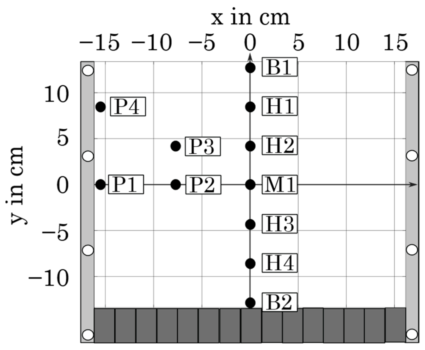
4.1. System Alignment

Before conducting measurements using the MIMO system, it was essential to perform a system alignment to ensure accurate particle localization. Note that the coordinate system for the radar imaging was spanned with respect to the centre of the measurement set-up. Furthermore, it was crucial to know the precise positions of the antennas relative to the reactor walls, as the value was used for backprojection and refraction compensation. To achieve this, cross-line lasers were employed to position the grate system precisely at the centre of the ring structure. This process guaranteed symmetrical alignment. However, it is important to note that the physical distance established with the reactor walls did not correspond to the exact measurement distance of the electromagnetic wave. The decisive factor for the distance between the antenna and the reactor wall was the distance with respect to the phase centre inside of the antenna. Since it was not feasible to directly measure the phase centre of the antenna, reference measurements were necessary. As such, in order to achieve an unambiguous reflection behaviour, the walls of the container were replaced by metallic plates for system alignment. In contrast to the PC reactor walls, the reflection at a metal plate can be clearly assigned to the surface, while the PC reactor walls can be penetrated by the wave. By taking reflection measurements with all six antennas, the mean distance to the reactor walls was found as 0.484 m.

4.2. Optical Evaluation

The determination of the particle positions using the images of the digital camera was performed numerically in Matlab®. First, the images were straightened using a digital grid and optical distortions were compensated. Furthermore, all images were cropped to the same image area, which in this case corresponded to the front wall of the generic grate. It had to be ensured that all image sections were scaled to the same dimension in pixels, as this formed the reference size for determining the position in the following. The routine used to identify particle positions by identifying the particle centres in digital images is presented in [27]. The coordinate origin was placed in the centre of the particle with the position M1 (see Figure 8). This resulted in relative particle coordinates of the tracer particle for each image. For the current system with resting particles, the optical determination of tracer particle position would not have been mandatory; measurement with a metering rule would be sufficient. However, it is a preparatory step for measurements of an agitated particle assembly in future work.

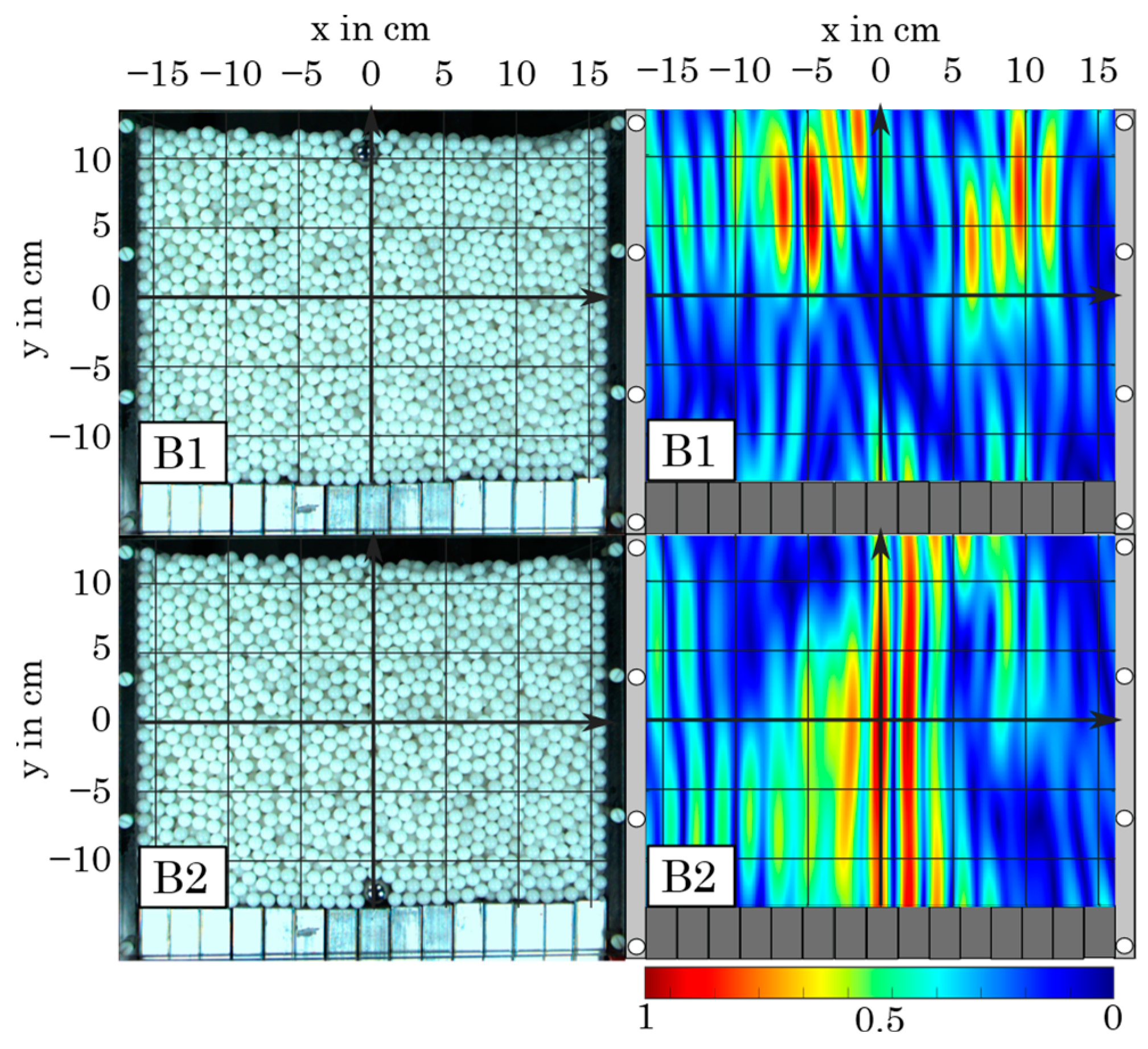
4.3. Measurement Results

In the following, a total of 11 different positions were recorded at different vertical and horizontal positions. Figure 8 shows the view of the reactor wall as seen from the camera with the corresponding marker positions. The following discussions refer to the labelling in Figure 8. The selected positions were focused on one half of the measurement area, since the measurement system was symmetrical. Figure 9 shows the results of the imaging process for all positions except the positions B1 and B2 at the top and bottom of the reactor. The results of the two positions are discussed separately in Section 4.4. In Figure 9, the left side shows the optical image provided by the camera, while the right side contains the reconstruction by the radar system normalized to the maximum value.
Before comparing the results for particle location quantitatively some explanations for the appearance of the radar images are given, focusing on position M1. The tracer particle was located in the centre position and can clearly be seen in the camera image. In the radar image, the location of the tracer particle corresponds to maximum intensity, indicated by the deep red colour. For clarity, the particle position is depicted by a black circle in the radar image. Visually, the particle position seems to be very similar in the camera image and the radar image. However, the radar image shows a 2D colour scheme with some vertical stripes.
Let us concentrate on the central stripe with the marker particle in its centre. This 2D pulse in the imaging plane is significantly wider than the marker particle and, furthermore, it can be noted that the 2D pulse is much wider in height than in width. This can be explained by the fact that the antennas were located in pairs on a ring, whereby the width was imaged by a circular aperture, while the height was computed by means of a linear aperture, since the antennas were arranged one above each other. As was shown in [33] for apertures in free space, the achievable resolution Δ c i r c of a circular aperture can be found as Δ c i r c = 2 π 2.4 λ c , while the resolution of a linear aperture is Δ l i n = λ c R 2 L . Here, λ c denotes the wavelength at the center frequency of the chirp signal, R denotes the distance between the aperture and the target, and L is the length of the linear aperture that corresponds to the distance between the two antennas in our set-up. By forming the ratio of the two equations, we find Δ l i n = R L π 2.4 Δ c i r c R L 1.31 Δ c i r c . For our set-up, we know that the distance between antenna and reactor is R = 0.484 m, while the distance between the two antennas is L = 0.123 m. Therefore, Δ l i n > Δ c i r c applies to our set-up, resulting in a widening of the pulse in height. For the results at position M1 in Figure 9, the resolution in height can be calculated as Δ h e i g h t = 11.4 cm, while the system provides a resolution of Δ w i d t h = 1 cm in width. This problem can be fixed by mounting more antennas in the vertical direction which will increase L and can be easily realized for larger reactors. Since we localized a single particle, this problem was not relevant as we were only interested in the maximum value: the marker particle position. In addition to the widening of the reconstructed target, it can be seen that there is an increased amount of clutter in the image next to the actual reconstructed target. This can be attributed to the effects of an undersampled aperture and multiple reflections within the bulk material. The effect of undersampling is well known from the field of radar imaging in free space applications, for instance linear apertures require an antenna spacing of λ m i n 2 , with the minimum wavelength λ m i n corresponding to the highest frequency. For a maximum frequency of 8.5 GHz, this results in an antenna spacing of approximately 1.76 cm. This is significantly smaller than the antenna spacing used in this work. If the required spacing is exceeded, this results in systematic artefacts in the image. In Figure 9, the effect of undersampling is noticeable through further ghost targets next to the actual target, which are, however, less pronounced in their amplitude. Due to the asymmetric resolution of the system already discussed, these appear as vertical stripes superimposed on the actual target. The effect of multiple reflections on the other hand was already discussed previously in terms of the signal processing procedure in Appendix E. The particles used in this work do not behave completely homogeneously and therefore lead to multiple reflections which result in random background noise in the image. In the following, the localization by the optical evaluation and the radar system will be compared. Figure 9 depicts a good qualitative agreement between the position localised by radar and by the camera. Table 1 gives a quantitative comparison. The table shows the distances of particle displacements between each position in comparison to position M1 at the centre of the reactor. As can be seen, the positions found by the optical and radar-based evaluation are close to each other for the great majority of all results. The exception is position H4, which appears to be 2.98 cm below the true position of the marker. The reason for this can be found in the fact that the particle is located close to the metallic bottom wall of the reactor. From electromagnetic theory it can be shown that the wave impedance between two metallic aluminium objects deviates from the free space wave impedance and increases with decreasing distance. For this reason, the marker can no longer be assumed to be a spherical target for the electromagnetic wave. Reflections can, therefore, also occur between the sphere and the metal wall, causing a virtual shift of the particle position in the radar evaluation. Position H4 was therefore excluded from further consideration. For the other measurement points, the deviation in localized position in x-direction between the optical and radar-based evaluation is in the interval of Δ x   0.31 ,   0.13 cm, with a standard deviation of σ x = 0.17 cm. On the other hand, the localization error in y–dimension is in the range of Δ y   1.33 ,   1.49 cm with a standard deviation of σ y = 0.86 cm.
Obviously, the localization by the radar system is worse in y-direction than in x-dimension. Here, the two positions H1 and P1 stand out, which show a deviation of + 1.49 cm and 1.33 cm, respectively. However, it must be taken into consideration that a sphere with a diameter of 2 cm was used as marker. Ideally, the camera evaluates the centre point of the sphere, but for the radar the marker appeared as a spatially extended target, whereby deviations of up to the radius of 1 cm are acceptable. When the results are compared with existing methods, commercially available CT and MRI systems [34] with a spatial resolution of less than one millimetre are significantly better. However, they are not suitable for real-time particle tracking due to their long measurement times. Methods such as PEPT [35], RPT [36], and MPT [37] have a resolution in the range of 1–2 mm and are also real-time capable, but PEPT and RPT cannot be used in industrial facilities. MPT systems are competitive systems, but particle synthesis is much more complicated than in a radar-based approach. With regard to the resolution of the system, it was shown previously that the resolution in the y-direction is worse by a factor of 11.4 , due to the arrangement of the antennas. This causes a decrease in localization accuracy in the y-direction, as the generated pulse after the imaging procedure is flatter than in the x-direction, making it more vulnerable to misplacements of the maximum value. Again, since the imaging procedure can be applied to the entire reactor, this is a general result that can also be found for a three-dimensional reconstruction of the volume.

4.4. Localization Limitations

In the following, the results for the positions B1 and B2 at the top and bottom of the reactor will be discussed. Figure 10 shows the respective imaging results of the radar system on the right and the camera images on the left.
Figure 10 shows that the radar system does not allow for a clear localization of the marker for the positions B1 and B2. The radar proposes the marker at 4.7,6.5 cm for position B1 and 0,0 cm for position B2, respectively. However, when compared with the camera pictures on the left, both positions are obviously wrong.
This can be explained by faulty assumptions in the signal processing procedure. For the range compression and backprojection, it was assumed that the marker was embedded in a homogeneous background material. This presupposes that there are no jumps in permittivity around the marker, i.e., that the marker lies in the middle of a certain volume that is completely filled with granulate. This assumption is not applicable for both positions as they are located at material boundaries. For instance, for the case of B1, there is only one layer of bulk material above the marker particle. For this, dielectric mixing formulas and the according assumptions for wave propagation are no longer valid. It is to be assumed that the wave propagates faster at the boundary than in the granular material, since air has a relative permittivity of ε r 1 and, therefore, the velocity at the surface will be close to the speed of light. For B2, basically the same argument holds true as for position H4, as discussed in the previous section.
The results imply that zones at the top and bottom of the reactor cannot be imaged by the radar signal processing proposed in this work and we refer to this region as shaded regions. Those regions have to be treated separately in future work, for instance by modelling the wave propagation at the boundary numerically by means of full-wave simulations.

5. Conclusions

In this work, we have introduced a radar-based system featuring six antennas, which allow for localisation of resting spherical marker particles within a generic grate system filled with polyoxymethylene particles. The key features of this system include its compatibility with non-intrusive particle localization, even within complex reactor geometries, while providing impressive spatial resolution.
The antennas were arranged in three pairs on a ring with a distance of 60 cm to the polycarbonate reactor side walls. The position of the antenna pairs was shifted by 90° in circumferential direction. Two antennas were always arranged on top of each other in order to obtain a spatial resolution in vertical direction. The measurements were carried out by applying the Frequency Modulated Continuous Wave principle using a vector network analyser as a signal source and a switching matrix for time multiplexing, whereby each channel was measured after another. To localize the marker particle inside the grate system, we introduced a radar imaging algorithm that enabled compensation for the wave refraction at the reactor walls and in the bulk material. Therefore, the proposed system is capable of localizing marker particles without mechanically interacting with the reactor walls, which allows the system to locate marker particles in reactors without disturbing the process inside. Finally, the system was evaluated by placing a metal sphere with a diameter of 20 mm in front of the reactors’ transparent wall, which enabled an alignment with an optical measurement by a digital camera. The evaluation shows that the position of the marker particle can be determined with a standard deviation of σ v e r t = 0.86 cm in the vertical direction and σ h o r = 0.17 cm in the horizontal direction, which is a promising result. However, it should be noted that the deviation in vertical direction can be improved for reactors with larger dimensions in vertical direction, since this allows to span larger apertures, improving spatial resolution. Compared to existing MIMO sensor concepts, this work successfully demonstrated the localization of markers in non-homogeneous granular media, even with significant undersampling and minimal hardware cost. We achieved effective three-dimensional imaging of the measurement area, paving the way for scalability to larger industrial plants. Furthermore, different regions of detection capability were identified. For future work this issue can be solved by modelling the propagation behavior of electromagnetic waves at material boundaries by means of full-wave simulations.
In future work, the goal is to track moving particles inside a granular assembly. Therefore, we will adapt the presented measurement principle. The measurements in the time-multiplex mode will be replaced by a parallel measurement of all receiving channels. The presented signal processing procedure can be also transferred to tracking applications in larger reactors without loss of accuracy as long as the number of antennas is scaled. To improve the accuracy in a tracking scenario, the method will be extended by applying, for instance, Kalman filters, which allow for a better estimation of the actual trajectory from the localised positions. The tracking system will then be applied to the generic grate system, which allows for mechanical agitation of the particle assembly. For this, the aluminum bars at the bottom will be replaced by bars made of plastic, to allow for a precise localization of the particles at the bottom of the grate.
In conclusion, our work opens up new possibilities for non-intrusive particle localization and tracking within complex granular assemblies. This technology has the potential to be used in various applications in mechanical process engineering, offering enhanced control and understanding of particle movement in industrial systems.

Author Contributions

Conceptualization, J.S. and F.S.; methodology, J.S., F.S. and N.H.; software, J.S.; validation, J.S., F.S. and N.H.; formal analysis, J.S.; investigation, J.S. and F.S.; resources, J.S.; data curation, F.S.; writing—original draft preparation, J.S.; writing—review and editing, J.S., F.S. and N.H.; visualization, J.S. and F.S.; supervision, C.S. and J.B.; project administration, I.R. and V.S.; funding acquisition, I.R. and V.S. All authors have read and agreed to the published version of the manuscript.

Funding

This research was funded by the Deutsche Forschungsgemeinschaft (DFG, German Research Foundation), grant number 422037413–CRC/TRR 287 “BULK-REACTION”.

Data Availability Statement

Data are contained within the article.

Conflicts of Interest

The authors declare no conflict of interest.

Abbreviations

Latin Symbols
SymbolUnitDenotation
B[Hz]bandwidth
c [m/s]wave velocity
c 0 [m/s]speed of light
f [Hz]frequency
h [m]vertical distance
I _ x , y complex image
J F Θ Jacobian matrix
L[m]distance between two antennas
M number of transmitters
N number of receivers
n refraction index
R[m]object distance
R x receiver
s T x ( t ) transmission signal
s R x ( t ) received signal
s I F ( t ) intermediate frequency (IF-) signal
T[s]end of time interval
T x transmitter
W [m]horizontal distance between antenna and target
w [m]variable
x p [m]particle position x-direction
y p [m]particle position y-direction
Greek Symbols
SymbolUnitDenotation
α [rad]angle of incidence
[m]resolution
Δ c i r c [m]circular aperture
Δ f [Hz]angular frequency
Δ l i n [m]linear aperture
ε r relative permittivity
λ [m]wavelength
μ r permeability
σ standard deviation
τ [s]the round-trip time
ϕ [rad]phase shift
AbbreviationDenotation
MIMOmultiple-input multiple-output
MRImagnetic resonance imaging
MPTmagnetic particle tracking
PEPTpositron emission particle tracking
FMCWfrequency modulated continuous wave
RPTradioactive particle tracking
POMpolyoxymethylene
VNAvector network analyzer
LPlow-pass filtered
IFintermediate frequency
PCpolycarbonate

Appendix A

In this work, we deal with an FMCW radar which emits a linear frequency modulated chirp signal with a certain bandwidth B over a time period T . Therefore, the signal s T x t is chosen as a harmonic oscillation with a linear increasing frequency during the time interval t 0 , T . For a frequency varying in the interval f f m i n , f m a x , one can formulate a simple linear correlation between time t and frequency f t as follows:
f t = f m i n + B t T   ,   t 0 , T ,
Subsequently, the transmitted signal is found by calculating the phase ϕ t of the emitted wave and inserting the phase term into a harmonic oscillation. The phase can be derived from the known relationship between frequency and phase as ϕ t = 0 t f t d t = f m i n t + B t 2 2 T + ϕ 0 and the emitted high frequency signal is s T x t = a cos 2 π ϕ t . Here, a denotes an amplitude value that depends on the power the system can provide. However, since the amplitude of the emitted signal is not of interest for the general signal processing, it will be neglected in the following.
Regarding Figure 1, the emitted wave propagates in free space with the speed of light c 0 and hits the target at distance R . The target leads to a reflection of the wave and the reflected wave is recorded at the same antenna as in the transmitting case. This leads to a received signal, which is detected with a time delay of τ = 2 R c 0 , whereby the received signal states as s R x t = cos 2 π ϕ t τ .
Figure A1. Time dependent frequency profile of the emitted and received wave, respectively.
Processes 11 03183 g0a1
Figure A1 shows the profile of the frequency over time, starting at a minimum frequency f 0 = f m i n and approaching the maximum value f T = f m a x with f m a x f m i n being the bandwidth B. Here, the blue path represents the frequency of the emitted signal and the green path denotes the received signal. Obviously, the blue signal is shifted by a delay τ . It shows that the system converts the time delay of the signals into a frequency difference Δ f . By applying the intercept theorem, one finds the relationship Δ f B = τ T . Therefore, the time delay τ   can be determined unambiguously by finding the intermediate frequency Δ f . In practice, this is realized by multiplying the time domain signals s T x t and s R x t . From Fourier theory, it is known that a multiplication in time domain leads to a shift in frequency domain. Assuming two cosine-shaped signals with a frequency of f and multiply them by each other, the following relationship is valid:
cos 2 π f 1 t cos 2 π f 2 t = cos 2 π f 1 + f 2 t + cos 2 π f 1 f 2 t ,
Therefore, a multiplication of the emitted and received signal in the mixer and suppressing the sum frequency with a low-pass filter produces a signal with a constant frequency Δ f = f 1 f 2 . Recalling the found formulas for the received signal and the emitted signal and focusing on the lower band selected by the LP, the intermediate frequency signal can be found as
s I F t = cos 2 π Δ f t + ϕ t , t 0 , T

Appendix B

In general, an FMCW radar is capable of detecting multiple targets. However, as already stated, the resolution of a radar is limited by its bandwidth B . The intermediate frequency signal s I F t provides only a limited extension in time and frequency. This corresponds to a multiplication of an infinitely long signal with a rectangular function of length T . As it is known from theory, the Fourier transformation of a harmonic oscillation corresponds to an infinitely small pulse in frequency domain. However, it can be shown that the symmetrical defined rectangle function of length T transforms as F r e c t t T f = T s i n c T f . Therefore, applying the Fourier transform on s I F t leads to s i n c -pulses with a finite pulse width, limiting the resolution of the system at which two targets can be separated unambiguously. In fact, it can be shown that the s i n c -pulses tend to smear when the spatial distance between the targets drops under a value of Δ R = c 0 2 B .

Appendix C

The general procedure of the imaging problem is shown in Figure A2 for a total of M transmitters and N receivers.
Figure A2. Procedure of the backprojection algorithm for a total of M transmitters, N receivers and L pixels.
Processes 11 03183 g0a2
As the input, the algorithm requires the range-compressed signals S as well as the antenna positions. In the first step, a 2D-grid I with a total of L pixels is formed, where each pixel is assigned to a certain position in space. Afterwards, one must iterate over the transmitting and receiving antennas, to account for each possible combination of antennas. In the given procedure, the first loop iterates over the M transmitters. For each transmitter, the second inner loop iterates over the N receiver positions and the third loop accounts for the L pixels. In the main part, the distance between the l -th pixel and the m -th transmitter or n -th receiver is calculated, which is denoted as R t r , 1 or R t r , 2 , in reference to Figure 2. If these values are found, the overall distance is R = R t r , 1 + R t r , 2 and the value in the range-compressed signal S associated with the pixel is found by S R . The range-compressed signal is complex valued and therefore, to compensate for the phase shift, the found value must be multiplied with the complex conjugate e j 2 π f m i n R c . The algorithm ends after repeating the procedure for all possible combinations of receivers and transmitters. The output is a complex-valued image, where the coordinates of the pixels are known due to the calculation.

Appendix D

The problem in (5) cannot be solved analytically, however, the solution for this type of problem can be effectively approximated using Newton’s Iteration. For this, the Jacobian matrix J F Θ is required that can be found by differentiation of (5). In the following, only the solution for J F Θ is shown, a derivation is omitted here.
J F , 1 Θ = w 1 + w 3 W W w 1 w 3 2 + h 2 2 w 1 3 1 + h 1 w 1 2 1 2 0 0 w 3 3 1 + h 3 w 3 2 1 2
J F , 2 Θ = W w 1 w 3 W w 1 w 3 2 + h 2 2 3 2 1 W w 1 w 3 + h 2 2 1 2 1 + h 1 w 1 2   1 + h 1 w 1 2   1 + h 3 w 3 2   1 + h 3 w 3 2   ,
J F Θ = J F , 1 Θ + J F , 2 Θ ,
With the function F Θ and the Jacobian matrix J F Θ known, the iteration rule of the Newton method states as
Θ n + 1 = Θ n J F Θ n 1 F Θ n ,
The presented method will converge to the root of (5) until a certain criterion for convergence is met. For instance, one can define an acceptable residual error e . From the definition of convergence, there exists an N , so that Θ n + 1 Θ n 2 < e     n > N .

Appendix E

Inverting a measurement to receive range information requires an accurate modelling of the wave propagation. In Section 2, the assumption was that the wave propagates in a homogeneous material with a well-defined relative permittivity. However, in the given problem setting, the material is not a continuum but consists of spherical particles. For the case of inhomogeneous materials, it was shown in [38] that media consisting of a material with small inclusions behave like a continuum, with an effective permittivity given by dielectric mixing models. However, mixing equations are only valid as long as particles are small against the wavelength. For the given measurement set-up and a particle size of 10 mm, it must be assumed that the material behaves inhomogeneously, especially for the high frequency components of the emitted frequency ramp, whereby reflections occur within the medium. Therefore, it can be assumed that the bulk material offers a constant propagation speed on average, but the surrounding bulk material cannot be assumed to be completely homogeneous, leading to clutter in the processed images. For the given granular material, the effective permittivity for signal processing was found as ε r , p = 2.05 and therefore, the velocity of the wave can be assumed as c = c 0 ε r , p inside the bulk material. Since the permittivity of the reactor wall was already found as ε r = 2.57 and all geometrical properties of the system are known, the round-trip time of a wave propagating from the antenna in free space to the particle inside the reactor can be calculated by Equation (5) and the numerical method in Appendix D.

References

  1. Di Renzo, A.; Rito, G.; Di Maio, F.P. Systematic Experimental Investigation of Segregation Direction and Layer Inversion in Binary Liquid-Fluidized Bed. Processes 2020, 8, 177. [Google Scholar] [CrossRef]
  2. Piringer, H. Lime Shaft Kilns. Energy Procedia 2017, 120, 75–95. [Google Scholar] [CrossRef]
  3. Yin, C.; Rosendahl, L.A.; Kær, S.K. Grate-firing of biomass for heat and power production. Prog. Energy Combust. Sci. 2008, 34, 725–754. [Google Scholar] [CrossRef]
  4. Zanoli, S.M.; Pepe, C.; Astolfi, G. Advanced Process Control for Clinker Rotary Kiln and Grate Cooler. Sensors 2023, 23, 2805. [Google Scholar] [CrossRef] [PubMed]
  5. Amon, A.; Born, P.; Daniels, K.E.; Dijksman, J.A.; Huang, K.; Parker, D.; Schröter, M.; Stannarius, R.; Wierschem, A. Preface: Focus on imaging methods in granular physics. Rev. Sci. Instrum. 2017, 88, 051701. [Google Scholar] [CrossRef] [PubMed]
  6. Pore, M.; Ong, G.; Boyce, C.; Materazzi, M.; Gargiuli, J.; Leadbeater, T.; Sederman, A.; Dennis, J.; Holland, D.; Ingram, A.; et al. A comparison of magnetic resonance, X-ray and positron emission particle tracking measurements of a single jet of gas entering a bed of particles. Chem. Eng. Sci. 2015, 122, 210–218. [Google Scholar] [CrossRef]
  7. Bolomey, J.-C.; Jofre, L. Three decades of active microwave imaging achievements, difficulties and future challenges. In Proceedings of the 2010 IEEE International Conference on Wireless Information Technology and Systems (ICWITS), Honolulu, HI, USA, 28 August 2010; pp. 1–4. [Google Scholar]
  8. Och, A.; Holzl, P.A.; Schuster, S.; Scheiblhofer, S.; Zankl, D.; Pathuri-Bhuvana, V.; Weigel, R. High-Resolution Millimeter-Wave Tomography System for Nondestructive Testing of Low-Permittivity Materials. IEEE Trans. Microw. Theory Tech. 2021, 69, 1105–1113. [Google Scholar] [CrossRef]
  9. Brooks, S.L. COMPUTED TOMOGRAPHY. Dent. Clin. N. Am. 1993, 37, 575–590. [Google Scholar] [CrossRef]
  10. Kawaguchi, T. MRI measurement of granular flows and fluid-particle flows. Adv. Powder Technol. 2010, 21, 235–241. [Google Scholar] [CrossRef]
  11. van de Velden, M.; Baeyens, J.; Seville, J.P.K.; Fan, X. The solids flow in the riser of a Circulating Fluidised Bed (CFB) viewed by Positron Emission Particle Tracking (PEPT). Powder Technol. 2008, 183, 290–296. [Google Scholar] [CrossRef]
  12. Rasouli, M.; Bertrand, F.; Chaouki, J. A multiple radioactive particle tracking technique to investigate particulate flows. AIChE J. 2015, 61, 384–394. [Google Scholar] [CrossRef]
  13. Buist, K.A.; van Erdewijk, T.W.; Deen, N.G.; Kuipers, J.A.M. Determination and comparison of rotational velocity in a pseudo 2-D fluidized bed using magnetic particle tracking and discrete particle modeling. AIChE J. 2015, 61, 3198–3207. [Google Scholar] [CrossRef]
  14. Kim, S.; Kim, J.; Chung, C.; Ka, M.-H. Derivation and Validation of Three-Dimensional Microwave Imaging Using a W-Band MIMO Radar. IEEE Trans. Geosci. Remote. Sens. 2022, 60, 1–16. [Google Scholar] [CrossRef]
  15. Jia, Y.; Cui, C.; Yan, C.; Zhong, X.; Guo, Y.; Chen, G. MIMO Through-Wall-Radar Spotlight Imaging Based on Arithmetic Image Fusion. In Proceedings of the 2018 21st International Conference on Information Fusion (FUSION 2018), Cambridge, UK, 10–13 July 2018; pp. 1498–1502. [Google Scholar]
  16. Wu, Z.; Wang, H. Microwave Tomography for Industrial Process Imaging: Example Applications and Experimental Results. IEEE Antennas Propag. Mag. 2017, 59, 61–71. [Google Scholar] [CrossRef]
  17. Kalender, W.A. X-ray computed tomography. Phys. Med. Biol. 2006, 51, R29–R43. [Google Scholar] [CrossRef]
  18. Panzner, B.; Jöstingmeier, A.; Omar, A. Computer tomography as imaging technique for ground penetrating radar A case study. In Proceedings of the 2012 14th International Conference on Ground Penetrating Radar (GPR), Shanghai, China, 4–8 June 2012; pp. 301–304. [Google Scholar]
  19. Gholamzadehmir, M.; Del Pero, C.; Buffa, S.; Fedrizzi, R.; Aste, N. Adaptive-predictive control strategy for HVAC systems in smart buildings—A review. Sustain. Cities Soc. 2020, 63, 102480. [Google Scholar] [CrossRef]
  20. Thormann, K.; Baum, M.; Honer, J. Extended Target Tracking Using Gaussian Processes with High-Resolution Automotive Radar. In Proceedings of the 2018 21st International Conference on Information Fusion (FUSION 2018), Cambridge, UK, 10–13 July 2018; pp. 1764–1770. [Google Scholar]
  21. Kumuda, D.K.; Vandana, G.S.; Pardhasaradhi, B.; Raghavendra, B.S.; Srihari, P.; Cenkeramaddi, L.R. Multitarget Detection and Tracking by Mitigating Spot Jammer Attack in 77-GHz mm-Wave Radars: An Experimental Evaluation. IEEE Sens. J. 2023, 23, 5345–5361. [Google Scholar] [CrossRef]
  22. Pearce, A.; Zhang, J.A.; Xu, R.; Wu, K. Multi-Object Tracking with mmWave Radar: A Review. Electronics 2023, 12, 308. [Google Scholar] [CrossRef]
  23. Laviada, J.; Wu, B.; Ghasr, M.T.; Zoughi, R. Nondestructive Evaluation of Microwave-Penetrable Pipes by Synthetic Aperture Imaging Enhanced by Full-Wave Field Propagation Model. IEEE Trans. Instrum. Meas. 2019, 68, 1112–1119. [Google Scholar] [CrossRef]
  24. Wu, B.; Gao, Y.; Laviada, J.; Ghasr, M.T.; Zoughi, R. Time-Reversal SAR Imaging for Nondestructive Testing of Circular and Cylindrical Multilayered Dielectric Structures. IEEE Trans. Instrum. Meas. 2020, 69, 2057–2066. [Google Scholar] [CrossRef]
  25. Fallahpour, M.; Case, J.T.; Ghasr, M.T.; Zoughi, R. Piecewise and Wiener Filter-Based SAR Techniques for Monostatic Microwave Imaging of Layered Structures. IEEE Trans. Antennas Propag. 2014, 62, 282–294. [Google Scholar] [CrossRef]
  26. Schorlemer, J.; Schulz, C.; Pohl, N.; Rolfes, I.; Barowski, J. Compensation of Sensor Movements in Short-Range FMCW Synthetic Aperture Radar Algorithms. IEEE Trans. Microw. Theory Tech. 2021, 69, 5145–5159. [Google Scholar] [CrossRef]
  27. Schorlemer, J.; Jebramcik, J.; Rolfes, I.; Barowski, J. Comparison of Short-Range SAR Imaging Algorithms for the Detection of Landmines using Numerical Simulations. In Proceedings of the 2021 18th European Radar Conference (EuRAD), London, UK, 5–7 April 2022; IEEE: New York, NY, USA, 2022; pp. 393–396. [Google Scholar]
  28. Hilse, N.; Kriegeskorte, M.; Illana, E.; Wirtz, S.; Scherer, V. Mixing and segregation of spheres of three different sizes on a batch stoker grate: Experiments and discrete element simulation. Powder Technol. 2022, 400, 117258. [Google Scholar] [CrossRef]
  29. Rickelt, S. Discrete element simulation and experimental validation of conductive and convective heat transfer in moving granular material. In Berichte aus der Energietechnik; Shaker Verlag: Aachen, Germany, 2011. [Google Scholar]
  30. Riddle, B.; Baker-Jarvis, J.; Krupka, J. Complex permittivity measurements of common plastics over variable temperatures. IEEE Trans. Microw. Theory Tech. 2003, 51, 727–733. [Google Scholar] [CrossRef]
  31. Givot, B.L.; Gregory, A.P.; Salski, B.; Zentis, F.; Pettit, N.; Karpisz, T.; Kopyt, P. A comparison of measurements of the permittivity and loss angle of polymers in the frequency range 10 GHz to 90 GHz. In Proceedings of the 2021 15th European Conference on Antennas and Propagation (EuCAP), Düsseldorf, Germany, 22–26 March 2021; pp. 1–5. [Google Scholar]
  32. Hattenhorst, B.; van Delden, M.; Schenkel, F.; Schorlemer, J.; Barowski, J.; Rolfes, I.; Musch, T. Tracer Particles with Encapsulated Resonators for Electromagnetic Localization and Tracking in Moving Bulk Materials; ICEAA: Venice, Italy, 2023. [Google Scholar]
  33. Batra, A.; Barowski, J.; Damyanov, D.; Wiemeler, M.; Rolfes, I.; Schultze, T.; Balzer, J.C.; Gohringer, D.; Kaiser, T. Short-Range SAR Imaging From GHz to THz Waves. IEEE J. Microw. 2021, 1, 574–585. [Google Scholar] [CrossRef]
  34. Koivukangas, T.; Katisko, J.; Koivukangas, J. Detection of the spatial accuracy of a magnetic resonance and surgical computed tomography scanner in the region of surgical interest. J. Med. Imaging 2014, 1, 015502. [Google Scholar] [CrossRef] [PubMed]
  35. Windows-Yule, C.R.K.; Seville, J.P.K.; Ingram, A.; Parker, D.J. Positron Emission Particle Tracking of Granular Flows. Annu. Rev. Chem. Biomol. Eng. 2020, 11, 367–396. [Google Scholar] [CrossRef]
  36. Dubé, O.; Dubé, D.; Chaouki, J.; Bertrand, F. Optimization of detector positioning in the radioactive particle tracking technique. Appl. Radiat. Isot. 2014, 89, 109–124. [Google Scholar] [CrossRef]
  37. Köhler, A.; Rasch, A.; Pallarès, D.; Johnsson, F. Experimental characterization of axial fuel mixing in fluidized beds by magnetic particle tracking. Powder Technol. 2017, 316, 492–499. [Google Scholar] [CrossRef]
  38. Sihvola, A.H.; Kong, J.A. Effective permittivity of dielectric mixtures. IEEE Trans. Geosci. Remote Sens. 1988, 26, 420–429. [Google Scholar] [CrossRef]
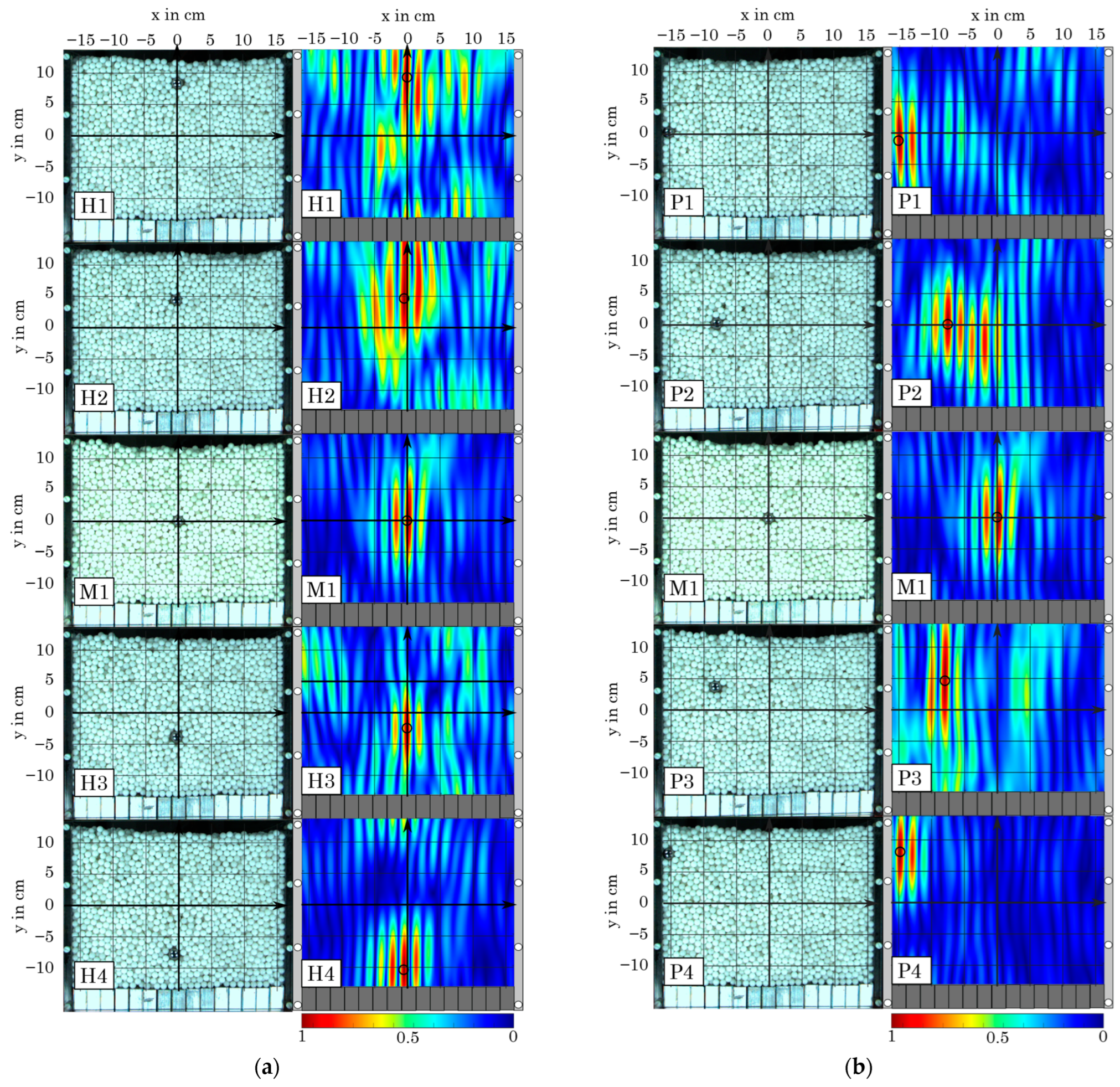
Figure 1. Basic set of an FMCW radar using a coupler to split the received and transmitted signal, enabling the system to work with only a single antenna.
Processes 11 03183 g001
Figure 2. Measurement scenario using a transmitter ( T x ) and a receiver ( R x ) to track a single particle.
Processes 11 03183 g002
Figure 3. Imaging result for a simulated point target at the center. The three antennas used for the imaging procedure are depicted in white and are located on a circle with a radius of 1 m. The image shows the absolute pixel values, normalized on the maximum value.
Processes 11 03183 g003
Figure 4. Refraction at a layered dielectric interface consisting of two layers with varying refraction indices n 2 and n 3 . The antenna emits an electromagnetic wave that is refracted at the two boundaries before hitting the target.
Processes 11 03183 g004
Figure 5. (a) Top view of the measurement setup and (b) a three dimensional sketch of the structure.
Processes 11 03183 g005
Figure 6. Image of the measurement set-up containing the generic grate system, the antennas as well as the camera and the spotlights.
Processes 11 03183 g006
Figure 7. Signal processing chain for the N input signals s I F , n and the empty measurement s ¯ I F . The output for the experimental measurements is a tupel of coordinates x p ,   y p in the imaging plane.
Processes 11 03183 g007
Figure 8. Marker particle positions as seen from the camera.
Processes 11 03183 g008
Figure 9. The left side shows the optical results provided by the camera, while the right side shows the reconstruction by the radar system using the backprojection algorithm. (a) Position H1, H2, M1, H3, H4. (b) Position P1, P2, M1, P3, P4.
Processes 11 03183 g009
Figure 10. Imaging results for the case that the particle approaches the upper or lower bound of the bulk material. The left side shows the image recorded by the camera; the right side shows the reconstruction of the radar.
Processes 11 03183 g010
Table 1. Particle displacements in comparison to position M1 for the optical evaluation with the camera and the radar system.
PositionParticle Displacement (Optical Evaluation)Particle Displacement (Radar-Based Evaluation)Difference in Particle Displacements
x in cmy in cmx in cmy in cm Δ x in cm Δ y in cm
M1------
H1−0.098.16−0.219.65−0.13+1.49
H2−0.224.49−0.534.6−0.31+0.11
H3−0.183.51−0.21−3.23−0.03−0.28
H4−0.49−7.3−0.63−10.72−0.14−2.98
P1−150.25−14.87−1.52+0.13−1.33
P2−7.70.38−7.590.35+0.11−0.03
P3−7.893.73−8.134.34−0.24+0.61
P4−157.59−14.877.53+0.13−0.06
Disclaimer/Publisher’s Note: The statements, opinions and data contained in all publications are solely those of the individual author(s) and contributor(s) and not of MDPI and/or the editor(s). MDPI and/or the editor(s) disclaim responsibility for any injury to people or property resulting from any ideas, methods, instructions or products referred to in the content.

