Mining and Analysis of Production Characteristics Data of Tight Gas Reservoirs

Abstract

The production characteristics of gas reservoirs are one of the important research subjects in gas reservoir development. To better guide the production development and strategy formulation of tight gas reservoirs, it is necessary to utilize data mining techniques to clarify the production characteristics of different reserves types of tight gas reservoirs. The production varies with the size of the recoverable reserves. In this study, 261 tight gas reservoirs worldwide were divided into three categories based on the size of their recoverable reserves. By considering the complete lifecycle of tight gas reservoirs, the production variations were classified into 16 production features, and these features were compiled into a dataset. Three algorithms, namely random forest, LightGBM, and CatBoost, were trained separately to analyze the relationship between the production characteristics and the size of the recoverable reserves of tight gas reservoirs. The objective was to define the production characteristics of tight gas reservoirs with different reserve sizes. Consequently, a set of production characteristic judgment rules that align with the size of the recoverable reserves of tight gas reservoirs was established. The findings revealed that LightGBM provided accurate predictions for the development characteristics of tight gas reservoirs with different reserve sizes. The production characteristics of large-scale tight gas reservoirs are as follows: the cumulative production at the end of the production increase phase ranges from 10 to 115.8 billion cubic meters, while the cumulative production at the end of the stable production phase ranges from 7.9 to 154.9 billion cubic meters. The peak production ranges from 2.3 to 3.8 billion cubic meters, and the decline period is estimated to last between 40 to 51 years. For medium-scale tight gas reservoirs, the production characteristics are as follows: the cumulative production at the end of the production increase phase ranges from 2.5 to 10 billion cubic meters, while the cumulative production at the end of the stable production phase ranges from 2.4 to 7.9 billion cubic meters. The peak production ranges from 0.8 to 2.3 billion cubic meters, and the decline period ranges from 20 to 40 years. As for small-scale tight gas reservoirs, the production characteristics are as follows: the cumulative production at the end of the production increase phase ranges from 0.1 to 2.5 billion cubic meters, while the cumulative production at the end of the stable production phase ranges from 0.2 to 2.4 billion cubic meters. The peak production ranges from 0.005 to 0.8 billion cubic meters, and the decline period ranges from 3 to 20 years. This study can provide potential references for the formulation of development technology policies for tight gas reservoirs and the assessment of reservoir production potential.

1. Introduction

Unconventional natural gas plays an increasingly important role in the long-term development of the natural gas industry. As one of the significant sources of unconventional natural gas, tight gas is widely distributed in major oil and gas basins worldwide, with a total resource volume of 210 × 10¹² m³, representing enormous exploration and development potential [1]. Therefore, the accelerated development of tight gas resources holds significant strategic significance for China’s unconventional natural gas energy sector. Tight gas reservoirs are characterized by extremely low porosity and permeability, making their development challenging and costly. With the continuous advancement of research and development of tight gas formations domestically and internationally, there has been extensive attention and study on the analysis of the development characteristics of tight gas reservoirs. To better guide the production and development of tight reservoirs, as well as the assessment of their production capacity, it is necessary to utilize data mining techniques to determine the production characteristics of different reserve types in tight reservoirs.

Currently, scholars have conducted explorations on the development characteristics of different types of reservoirs, achieving significant research results [2,3,4,5,6,7,8,9,10,11,12,13,14,15,16]. For instance, Jia Ailin et al. [2] analyzed the development characteristics of different types of carbonate gas reservoirs, classifying them into the fissure-cavity type, reef-beach type, karst weathering crust type, and layered dolomite type. Xu Zhengshun et al. [3] conducted tests and gas production studies on volcanic gas reservoirs, confirming their geological and dynamic development characteristics, and proposing a set of development strategies applicable to volcanic gas reservoirs in the region. Sun Laixi et al. [5] analyzed the development characteristics of the Jingbian gas field, recommending feasible production scale and steady production techniques, which provide a valuable reference for the development of the Jingbian gas field. Other researchers have also explored the development characteristics of different types of reservoirs, such as typical bottom-water reservoirs, the fourth member of the Dengying Formation in Anyue Gas Field, and deep, high-pressure carbonate gas reservoirs [6,7,8]. Jia Ailin et al. [15] conducted a study on the development characteristics of discovered giant gas fields globally and classified large reservoirs into five types. Li Jiudi et al. [16] comprehensively reviewed all developed gas fields and summarized the dynamic development and production characteristics exhibited by different types of reservoirs. The above scholars have analyzed the development characteristics and classification of different types of reservoirs, but few have studied the development characteristics of tight reservoirs. Therefore, this paper examined the development characteristics of tight gas reservoirs and explored the relationship between the variation in production characteristics and different reservoir sizes of tight gas reservoirs.

Machine learning is a method that employs intelligent algorithms to achieve autonomous learning, optimization, and prediction. Initially, machine learning found its application in the field of computer vision, with a focus on developing algorithms for image classification and pattern recognition. However, it has now been successfully deployed across various industries due to its ability to leverage diverse analytical methods and tools to establish models that extract key data and derive useful information from vast and complex datasets. In the realm of studying tight gas reservoir development characteristics, machine learning plays a crucial role. By learning from a large number of gas reservoir development characteristics, it can use various algorithms to build models. This allows for the identification of vital indicators influencing the development characteristics of tight gas reservoirs. Moreover, it facilitates the exploration of the intricate relationship between different types of tight gas reservoirs’ reserves and production characteristics. As a result, machine learning enables efficient gas reservoir classification, feature extraction, and consequently mitigates the challenges arising from the voluminous nature of the data involved. Yan Xingyu et al. [17] applied the XGBoost algorithm to the interpretation of well logging in tight sandstone gas reservoirs, and compared it with the random forest method and support vector machine method. The results showed that the XGBoost algorithm can accurately predict porosity and permeability, and effectively identify the tight sandstone gas reservoir in the study area. Nie Yunli et al. [18] proposed a shale gas “sweet spot” classification method based on random forest. By optimizing parameters and making predictions using a single decision tree and a random forest algorithm model, the classification prediction results of shale gas “sweet spots” are obtained. The results show that the random forest machine learning method can avoid the shortcomings of a single decision tree and is an effective means of identifying and predicting shale gas “sweet spots”. This paper applies data mining methods to the study of global tight reservoir development characteristics. Classification predictions are made using Boosting and Bagging models [19,20], which enhance the generalization ability of the models and avoid prediction defects caused by using a single model. Through comparative analysis of three ensemble models, it is concluded that the LightGBM model has the best predictive effect for different categories of tight reservoirs, and based on this, the relationship between production characteristics of tight reservoirs of different reserve sizes is determined through feature importance analysis.

Due to the limited data acquisition, this paper has some limitations in the selection of gas reservoir production characteristic parameters, which will be further improved in the future. Due to the scarcity of geological measurement data for global reservoirs, this study utilizes historical production data of global tight gas reservoirs to mine the development characteristics of reservoirs with different reserves. By exploring the implicit relationships among parameters throughout the reservoir’s lifecycle, the relationship between the size of reserves and the changes in production characteristics of tight gas reservoirs is analyzed, clarifying the production characteristics of reservoirs with different reserves.

In the study of the development characteristics of reservoirs, few scholars have investigated the relationship between reserves and production characteristics of tight gas reservoirs. Moreover, most existing research on reservoir development characteristics relies on individual models for prediction. Therefore, the innovation of this study lies in the exploration of the entire life cycle characteristics of 261 global tight gas reservoirs and the compilation of a dataset. Three different integrated models are introduced for comparative analysis, which avoids the shortcomings of using a single model and improves the performance of prediction models. It has been determined that the LightGBM model performs the best for predicting different categories of tight gas reservoirs. The study also analyzes the relationship between the production characteristics of tight gas reservoirs and their reserves based on different sizes of reserves, providing a clear understanding of the production features of tight gas reservoirs with different reserve sizes. The analysis of the relationship between global tight gas reservoir production characteristics and reserves can provide valuable references for the formulation of development technology policies, the establishment of appropriate production strategies, and the assessment of production potential in the production development of tight gas reservoirs.

2. Model Introduction

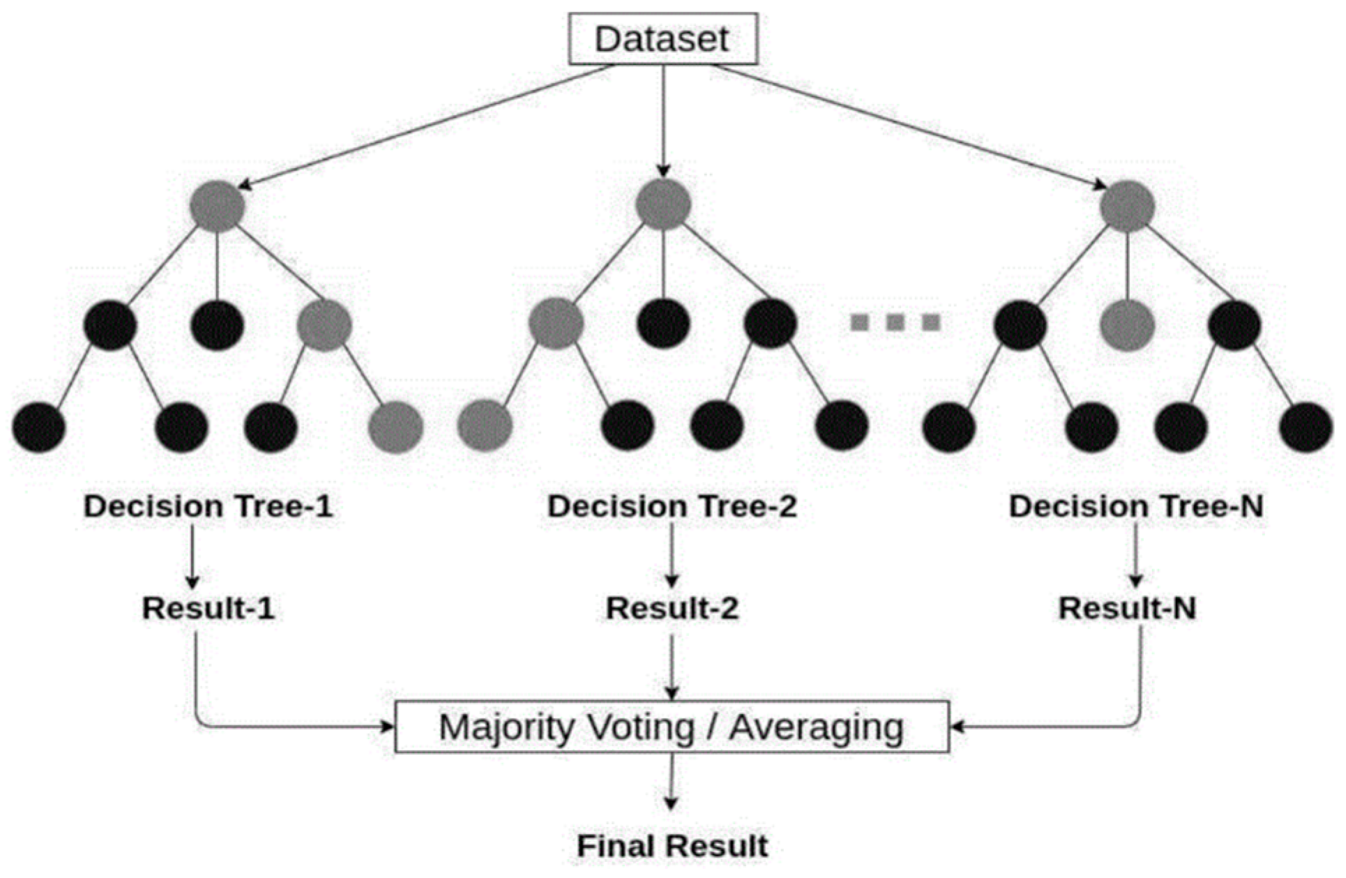
2.1. Random Forest

Random Forest is a nonlinear tree-based model that uses ensemble techniques to match multiple decision tree classifiers by majority voting or averaging the final results on different datasets. Random Forest is widely applied to classification and regression problems and has shown excellent performance in multi-class classification. Its main advantages lie in its ability to effectively handle high-dimensional data and large datasets, while also exhibiting good generalization ability and robustness [21].

Assuming there is a dataset D containing n samples: D = {($x_1$,$y_1$), ($x_2$,$y_2$), …, ($x_n$,$y_n$)}, where $x_n$ represents the feature vector of the n-th sample, and $y_n$ represents the corresponding label or prediction value, the training process is as follows:

(a)

Randomly select B features as the splitting features for each decision tree, constructing a randomly selected feature subset F;

(b)

Obtain a training set D_n of size n from the dataset D using sampling with replacement, where n is the size of D;

(c)

Build a decision tree model T_k using the feature subset F and training set D_n;

(d)

Repeat steps b and c until T decision trees are obtained.

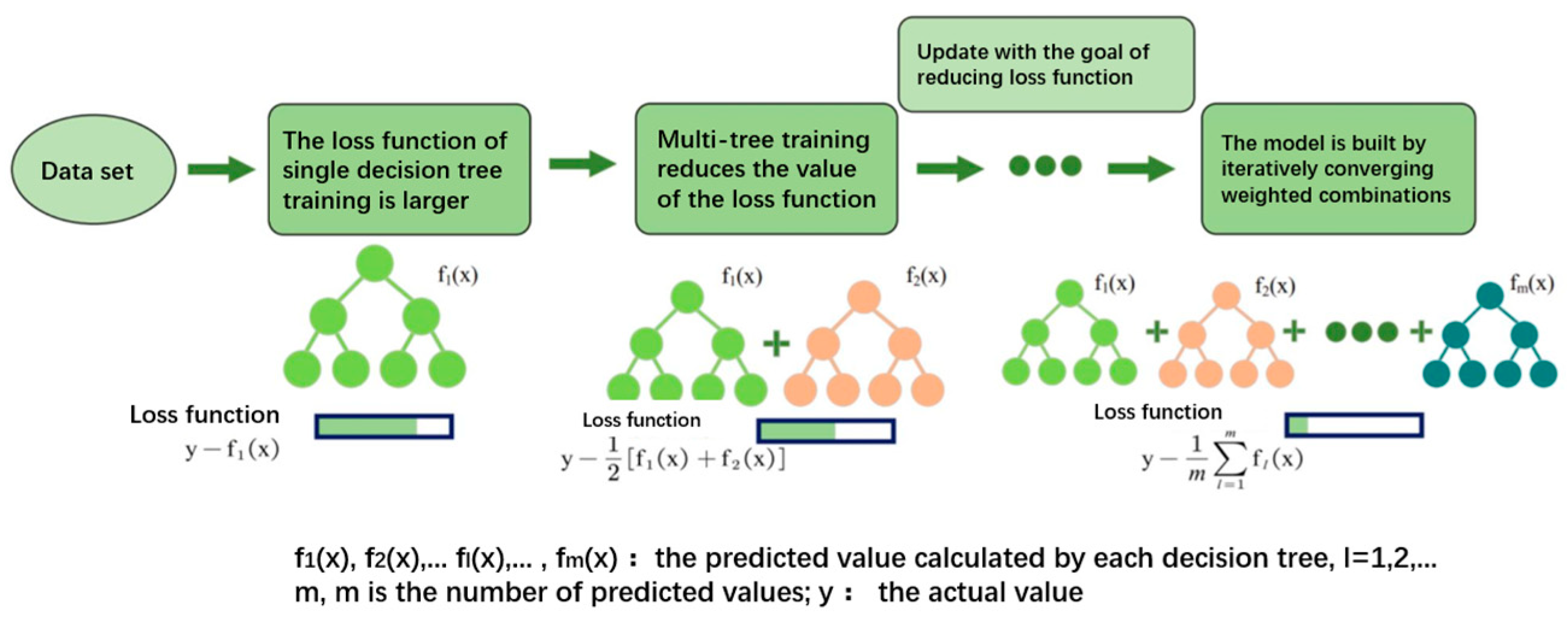
For classification problems, each decision tree T_k predicts a new sample x and produces a predicted class C_k. The final prediction result is determined by majority voting, selecting the class with the highest number of votes. For regression problems, each decision tree T_k predicts a new sample x and produces a predicted value V_k. The final prediction result is obtained by averaging the predicted values V_k of all decision trees (Figure 1).

2.2. LightGBM

Gradient Boosting Decision Tree (GBDT) is an additive model that accumulates the predicted values of all CART trees to obtain the final prediction. It iteratively trains the model by descending along the gradient of the loss function of the base learners. Let the training set be F = {($x_i$,$y_i$)${\}}_{i=1}^N$, where X = ($x_1$, $x_2$,…, $x_n$) represents the input sample features and Y = ($y_1$, $y_2$,…, $y_n$) represents the output sample features. The GBDT additive model can be represented as $f_m$(x) = $\sum _{m=1}^{M}T(x;{\theta }_m)$, where $T(x;{\theta }_m)$ represents a decision tree, ${\theta }_m$ represents the parameters of the decision tree, and M represents the number of trees.

LightGBM is an efficient classification model based on GBDT. It incorporates a series of optimization strategies to improve the training speed and accuracy of the model. It integrates Gradient-based One-Side Sampling (GOSS) and Exclusive Feature Bundling (EFB) techniques into GBDT, which enhances the training efficiency and reduces training time without compromising classification and regression accuracy. LightGBM not only prevents overfitting but also ensures high-performance models [22].

LightGBM employs a leaf-wise growth strategy to enhance model accuracy while reducing training data. The leaf-wise strategy involves iterating over all leaf nodes and computing the split gain for each leaf, and then splitting the leaf with the highest gain in each iteration. To prevent overfitting, LightGBM includes a maximum depth limit on top of the leaf-wise strategy [23,24] (Figure 2). Additionally, LightGBM utilizes a gradient-based one-sided sampling strategy. It retains all samples with higher gradients while randomly sampling from samples with lower gradients. By maintaining the same number of splits, the leaf-wise strategy can effectively reduce errors and achieve better accuracy.

2.3. CatBoost

CatBoost is an efficient classification model based on symmetric decision trees. It is suitable for addressing problems involving heterogeneous data, noisy data, and classification tasks. The objective of the CatBoost model is to minimize the loss function. Commonly used loss functions for classification problems include cross-entropy or exponential loss. Let L($y$,F) be the loss function, where y represents the true labels and F denotes the cumulative prediction of the model. The prediction of the CatBoost model is obtained by accumulating the results of decision trees. Assuming there are T decision trees, the model’s prediction is given by: $\mathrm{F}\left(x\right)=\sum (t=1to\mathrm{T})ft\left(x\right)$, where $ft\left(x\right)$ represents the prediction of the T-th decision tree and $x$ represents the input sample.

CatBoost has embedded an algorithm that automatically handles categorical features by converting them into numerical features. It leverages the relationships between features to create combinations of categorical features, significantly enriching the feature space. The model employs the Ordered Boosting method to counteract outliers in the dataset, mitigating bias and prediction offset. One of its main advantages is the utilization of an adaptive weighted strategy based on categorical features and an accelerated algorithm based on symmetric trees to improve the model. During each step of the decision tree computation, CatBoost adjusts the weights based on the residuals of the previous tree. This ensures that the current computation is conducted in the direction of the minimum residual from the previous computation, effectively avoiding bias and gradient bias [25]. Furthermore, CatBoost employs a gradient-based random greedy algorithm and a mean-based smoothing strategy to reduce the risk of overfitting and data waste (Figure 3). Firstly, the dataset is randomly shuffled. Then, the mean label value of samples with the same category is calculated. Finally, all categorical feature values are transformed into numeric results using the following formula. Let $\sigma =\left({\sigma }_1,\dots ,{\sigma }_n\right)$ be a random permutation, then $x_{\sigma j,k}$ is replaced by the expression given in Equation (1):

$$\frac{{\sum }_{j=1}^{p-1}\left[x_{\sigma j,k}=x_{\sigma p,k}\right]Y_{aj}+a·p}{{\sum }_{j=1}^{p-1}[x_{\sigma j,k}=x_{\sigma p,k}]+a}$$

(1)

In this formula, $p$ represents the prior value, and $a$ corresponds to the corresponding weight. The addition of prior values helps to reduce noise.

3. Classification Prediction

3.1. Dataset Introduction and Feature Selection

This study uses the global tight gas reservoir annual production data which were compiled by WOODMAC for the year 2022. Due to the general trend of gas reservoir production going through three stages: increasing, steady, and declining, this paper focuses on selecting the feature dataset based on these three stages.

The study identified a total of 261 tight gas reservoirs worldwide that possess full life cycle characteristics. Among these, 237 reservoirs are located in the Americas, with the majority situated in the United States. Following the Americas, there are eight reservoirs in Asia, seven in Africa, five in the Middle East, six in Europe, and one in the Central Asia-Russia region. The full life cycle characteristics of these 261 tight gas reservoirs were compiled into a dataset.

The 261 tight gas reservoirs are classified into large-, medium-, and small-size reservoirs based on their recoverable reserves [26,27,28]. The production characteristics of each stage, including production increase, stable production, and decline, are extracted from their annual production data and compiled into a dataset. The dataset consists of 17 feature variables and exhibits strong representativeness. By analyzing 16 production feature variables, including Initial production, Initial production time, End time of the production rising period, Final duration of yield increase., Cumulative output at the end of the period, Stable production period, Starting time of stable production, Stable yield, Accumulated output at the end of stable production, Declining years, Initial production decline, Peak yield, Time to peak production, Recovery degree, Storage and production ratio, and Gas recovery rate, the study aims to determine the size of recoverable reserves in the reservoirs and analyze the relationship between production features and different reserve sizes of tight gas reservoirs (

Table 1. Production characteristic variables of tight gas reservoirs.

	Characteristic Variable	Meaning and Unit
1	Initial production	Production data for the first year of field production (100 Million cubic meters)
2	Initial production time	Time of initial production of gas field (Year)
3	End time of production rising period	Point in time when gas field production stopped increasing (Year)
4	Final duration of yield increase	Total time spent on production upswing (Year)
5	Cumulative output at the end of the period	Cumulative production at the end of the upswing period (100 Million cubic meters)
6	Stable production period	Years of stable production period (Year)
7	Starting time of stable production	The time when the stable yield period begins (Year)
8	Stable yield	The average annual output during the stable production period (100 Million cubic meters)
9	Accumulated output at the end of stable production	Cumulative production at the end of a stable period (100 Million cubic meters)
10	Declining years	The duration of the decline period (Year)
11	Initial production decline	Production at the beginning of the decline period (100 Million cubic meters)
12	Peak yield	The maximum lifetime production of a gas field (100 Million cubic meters)
13	Time to peak production	The time when the field reaches maximum production (Year)
14	Recovery degree	The degree of production in the gas field (%)
15	Storage and production ratio	Reserve-production ratio of gas field
16	Gas recovery rate	Rate of gas production in a gas field (%)
17	Recoverable reserves	Recoverable reserves of gas fields (100 Million cubic meters)

).

Using the Seaborn library in Python, the correlation coefficients between the features are calculated, and a heatmap matrix is generated. For better visualization, the feature names are abbreviated by using their initials (Figure 4). The picture shows that the correlation between the features is strong, so the 16 features can be selected to predict tight gas reservoirs with different sizes of reserves.

3.2. Data Preprocessing

According to the full life cycle characteristics of each reservoir, the production characteristics at different stages of the historical production data were statistically analyzed and compiled into a dataset. Data checks were performed, including checking for missing values, outliers, data balance, and normalization [29].

The dataset was examined for missing values using the isnull() function in Python, and any outliers in the feature indicators were identified and removed. Due to the fact that the proportion of large-scale tight gas reservoirs in the total dataset is only 11%, the data are imbalanced. Therefore, in this study, the SMOTE oversampling technique was employed to balance the dataset. The SMOTE algorithm is a method for synthetic minority oversampling that creates new synthetic samples using the k-nearest neighbors algorithm to balance the dataset. This can reduce the tendency of the model to overfit and improve its robustness. However, its limitation is that it can potentially generate samples near the decision boundaries between the original samples. The results after balancing are shown in the following table (

Table 2. Statistical table of various gas reservoirs.

Type	Recoverable Reserves	Number of Original Datasets	Number of Datasets after Balancing
Large gas reservoir	More than 30 billion square meters	30	190
Medium gas reservoir	5 to 30 billion square meters	41	190
Small gas reservoir	0–5 billion square meters	190	190

). After balancing, the dataset was normalized. Then, the dataset was divided, with 70% of the data used as the training set, 20% as the testing set, and 10% as the validation set. To avoid encoding issues when conducting analysis using Python programming, feature discretization is performed. Large, medium, and small reservoirs are represented by 1, 2, and 3, respectively.

3.3. Model Selection and Implementation

In general, the prediction results of a single model may be biased to some extent. However, combining the results of multiple models often leads to better generalization performance than using a single model. Therefore, this study chooses to train an ensemble model [30]. Ensemble models can be divided into Bagging-based and Boosting-based models, depending on the ensemble method. Representative models of the Bagging-based approach include Random Forest, while representative models of the Boosting-based approach include XGBoost, LightGBM, and CatBoost. XGBoost, LightGBM, and CatBoost are currently considered state-of-the-art models, all of which are ensemble learning frameworks based on decision trees. XGBoost improves upon the original version of the decision tree algorithm (GBDT), while LightGBM and CatBoost further optimize upon XGBoost, each having their own advantages in terms of accuracy and speed. Therefore, this study selects Random Forest, LightGBM, and CatBoost as the three representative models.

Based on the principles of these models and the preprocessed data, modeling is conducted. First, using Python programming in PyCharm, Random Forest, LightGBM, and CatBoost models are trained and tuned. These three models have their own built-in hyperparameters. For example, max_depth represents the maximum depth of a tree, max_features represents the maximum number of features for an individual decision tree, min_samples_leaf represents the minimum number of samples required to be in a leaf node, min_samples_split represents the minimum number of samples required to split a node, and n_estimators represents the number of decision trees. Meanwhile, feature_fraction represents the feature fraction, learning_rate represents the step size of gradient boosting, num_leaves represents the specified number of leaves, and reg_lambda represents the weight of L2 regularization. Additionally, depth represents the maximum depth, and depth represents the L2 regularization parameter.

The optimal model is selected for prediction, and the classification results are analyzed. Therefore, this paper adopts the method of five-fold cross-validation and grid search for parameter optimization in classification prediction, and selects the specific value with better performance according to the performance of the model under different parameter values. Through mesh search tuning, the optimal combination of model parameters can be found, thus improving the performance and generalization ability of the model. The parameter ranges of mesh search tuning and the tuned hyperparameters are shown in the following table (

Table 3. Parameter ranges of three model grid search algorithms.

Random Forest	LightGBM	CatBoost
max_depth = [5, 10, 15, 20, None] max_features = [1, 2, 4] min_samples_leaf = [1, 2, 4] min_samples_split = [2, 5, 10] n_estimators = [10, 100, 200]	feature_fraction = [0.5, 0.8, 1] learning_rate = [0.01, 0.1, 0.3] max_depth = [−1, 3, 5, 8] n_estimators = [20, 40, 100] num_leaves = [16, 32, 64] reg_lambda = [1, 3, 5]	depth = [4, 6, 10] depth = [4, 6, 10] learning_rate = [0.01, 0.1]

and

Table 4. Hyperparameters of the three models after tuning.

Random Forest	LightGBM	CatBoost
Max_depth = 10 max_features = 4 min_samples_leaf = 2 min_samples_split = 10 n_estimators = 10	feature_fraction = 1 learning_rate = 0.3 max_depth = 3 n_estimators = 100 num_leaves = 16 reg_lambda = 1	depth = 4 l2_leaf_reg = 4 learning_rate = 0.01

). Then, under different optimized parameters for each algorithm, the accuracy, recall, and F1 scores on the classification model’s test set are used as the evaluation metrics for the model’s final performance.

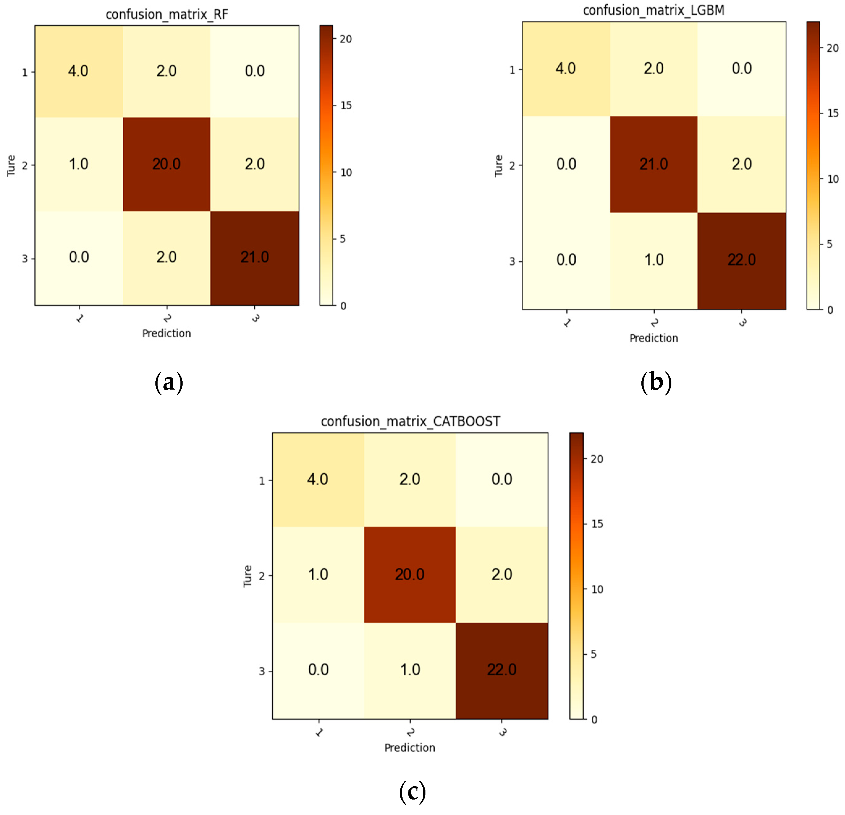
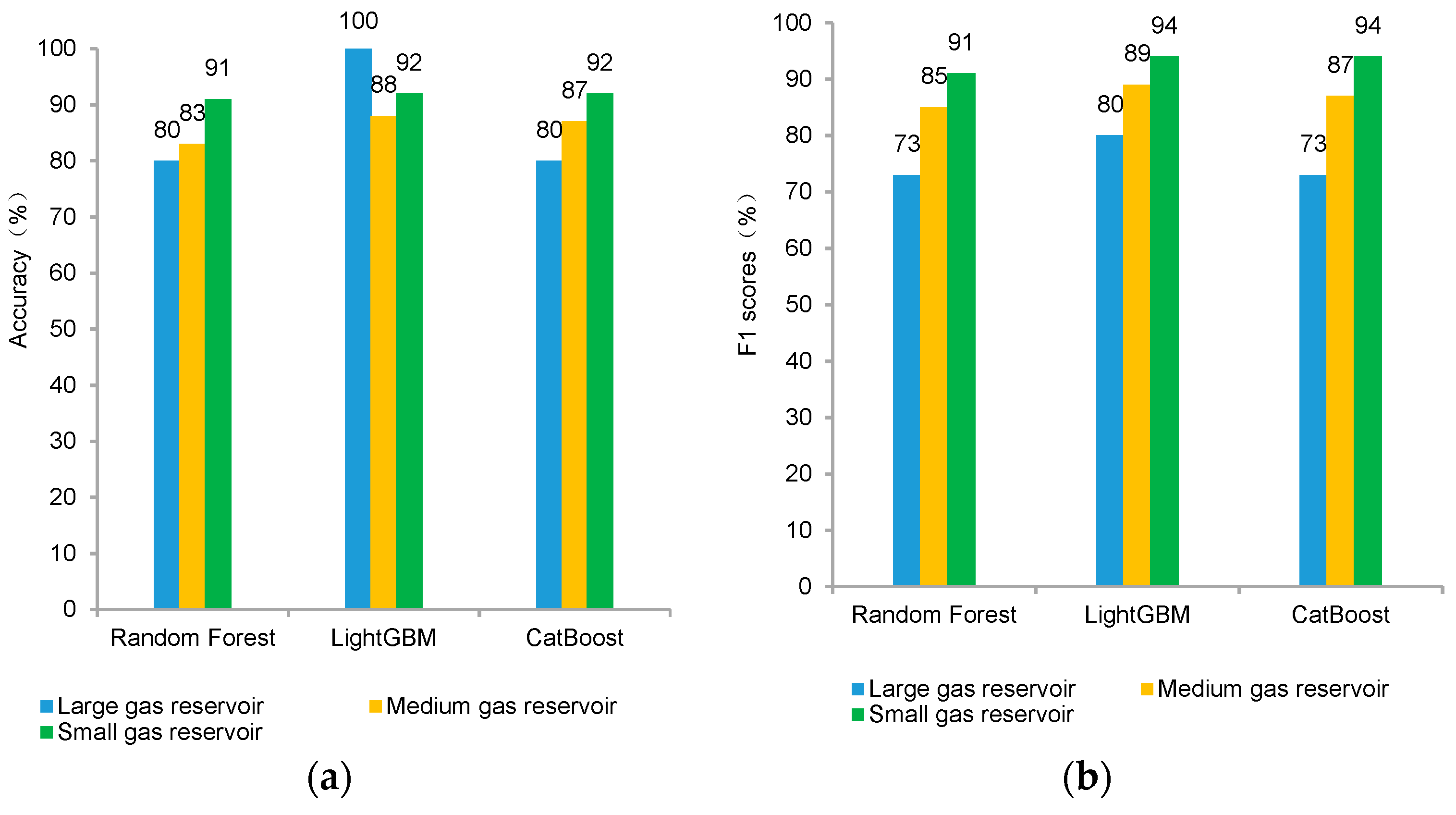
3.4. Comparative Analysis of Classification Models

The confusion matrix can compare the predicted results of a classification model with the true labels, showing the relationship between the prediction results of different classes. Multiple performance metrics, such as accuracy, precision, recall, and F1 score, can be calculated from the confusion matrix.

The 3 × 3 confusion matrix generated by the classification model reveals that on the test set, the random forest model correctly predicts four instances of large-scale reservoirs, while incorrectly predicting two instances. Additionally, there is one instance in which another class is incorrectly predicted as a large-scale reservoir. For medium-scale reservoirs, the model correctly predicts 20 instances, while incorrectly predicting three instances. Furthermore, there are four instances in which other classes are incorrectly predicted as medium-scale reservoirs. As for small-scale reservoirs, the model correctly predicts 21 instances, with two instances being incorrectly predicted. Moreover, there are two instances in which other classes are incorrectly predicted as small-scale reservoirs. the random forest model has accuracy rates of 80%, 83%, and 91% for large, medium, and small reservoir predictions, respectively. The corresponding recall rates are 67%, 87%, and 91%, and the F1 scores are 73%,85%, and 91%. The overall precision of the model is 87%. After analysis, it is found that the random forest model performs moderately well in predicting large and medium-sized tight reservoirs, but it has a better performance in predicting small tight reservoirs.

The CatBoost model correctly predicts four instances of large-scale reservoirs in the test set, while incorrectly predicting two instances. Additionally, there is one instance in which another class is incorrectly predicted as a large-scale reservoir. For medium-scale reservoirs, the model correctly predicts 20 instances, while incorrectly predicting three instances. Furthermore, there are three instances in which other classes are incorrectly predicted as medium-scale reservoirs. As for small-scale reservoirs, the model correctly predicts 22 instances, with one instance being incorrectly predicted. Moreover, there are two instances in which other classes are incorrectly predicted as small-scale reservoirs. The CatBoost model has accuracy rates of 80%, 87%, and 92% for large, medium, and small reservoir predictions, respectively. The corresponding recall rates are 67%, 87%, and 96%, and the F1 scores are 73%, 87%, and 94%. The overall precision of the model is 88%. Upon analysis, it can be observed that the CatBoost model exhibits high accuracy in predicting small and medium-sized tight reservoirs, but its accuracy in predicting large tight reservoirs is moderate.

In the test set, the LightGBM model correctly predicts four instances of large-scale reservoirs, while incorrectly predicting two instances. Additionally, there are zero instances in which other classes are incorrectly predicted as large-scale reservoirs. For medium-scale reservoirs, the model correctly predicts 21 instances, while incorrectly predicting two instances. Furthermore, there are three instances in which other classes are incorrectly predicted as medium-scale reservoirs. As for small-scale reservoirs, the model correctly predicts 22 instances, with one instance being incorrectly predicted. Moreover, there are two instances in which other classes are incorrectly predicted as small-scale reservoirs. The LightGBM model has accuracy rates of 100%, 88%, and 92% for large, medium, and small reservoir predictions, respectively. The corresponding recall rates are 67%, 91%, and 96%, and the F1 scores are 80%, 89%, and 92%. The overall precision of the model is 90%. After analysis, it is found that the LightGBM model has a good prediction performance for large, medium, and small tight reservoirs, with high F1 scores (Figure 5).

Through the comparison of the three models, it is concluded that the LightGBM model achieves the highest accuracy, performs well in terms of F1 scores for different types, and has the best prediction capability (Figure 6).

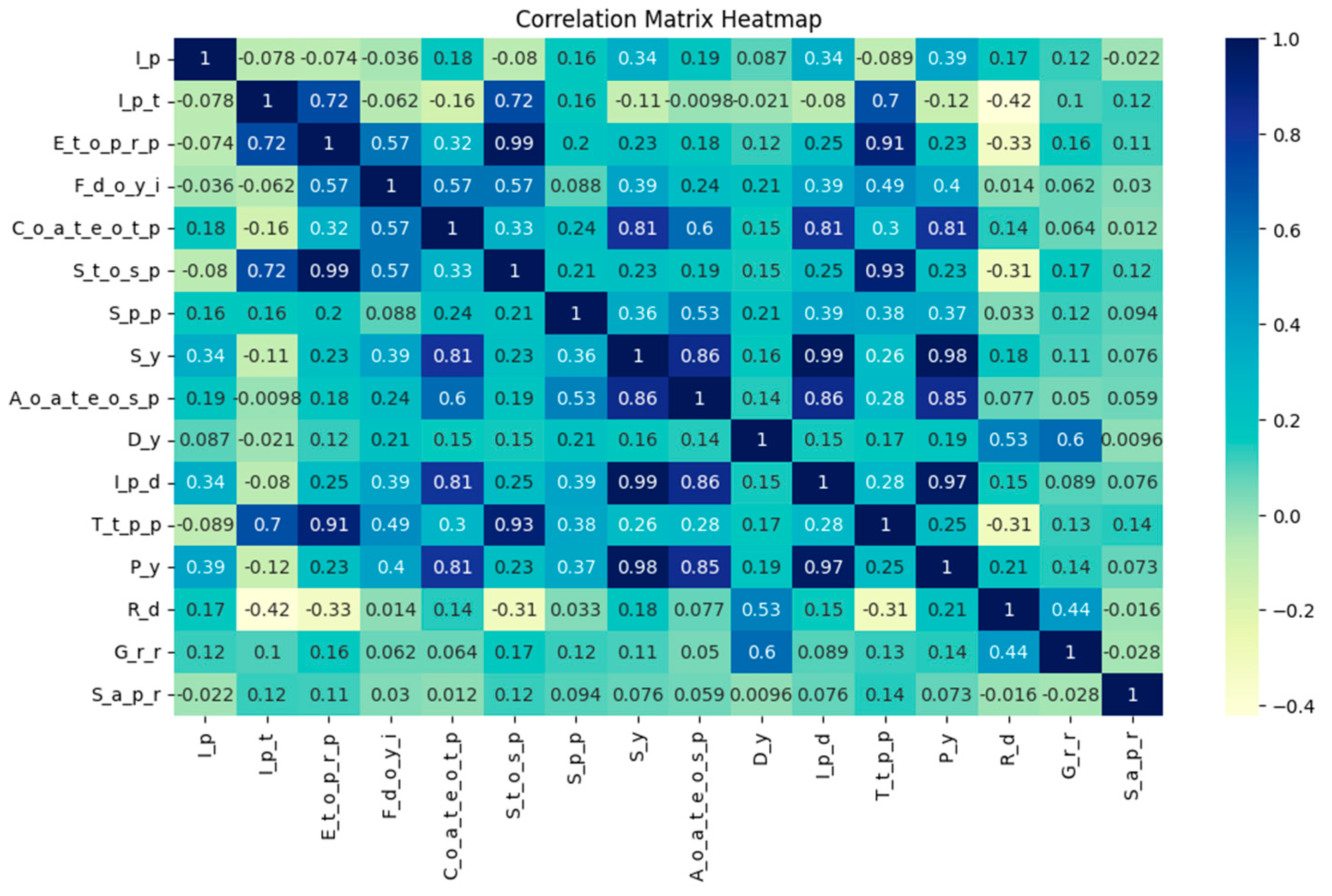
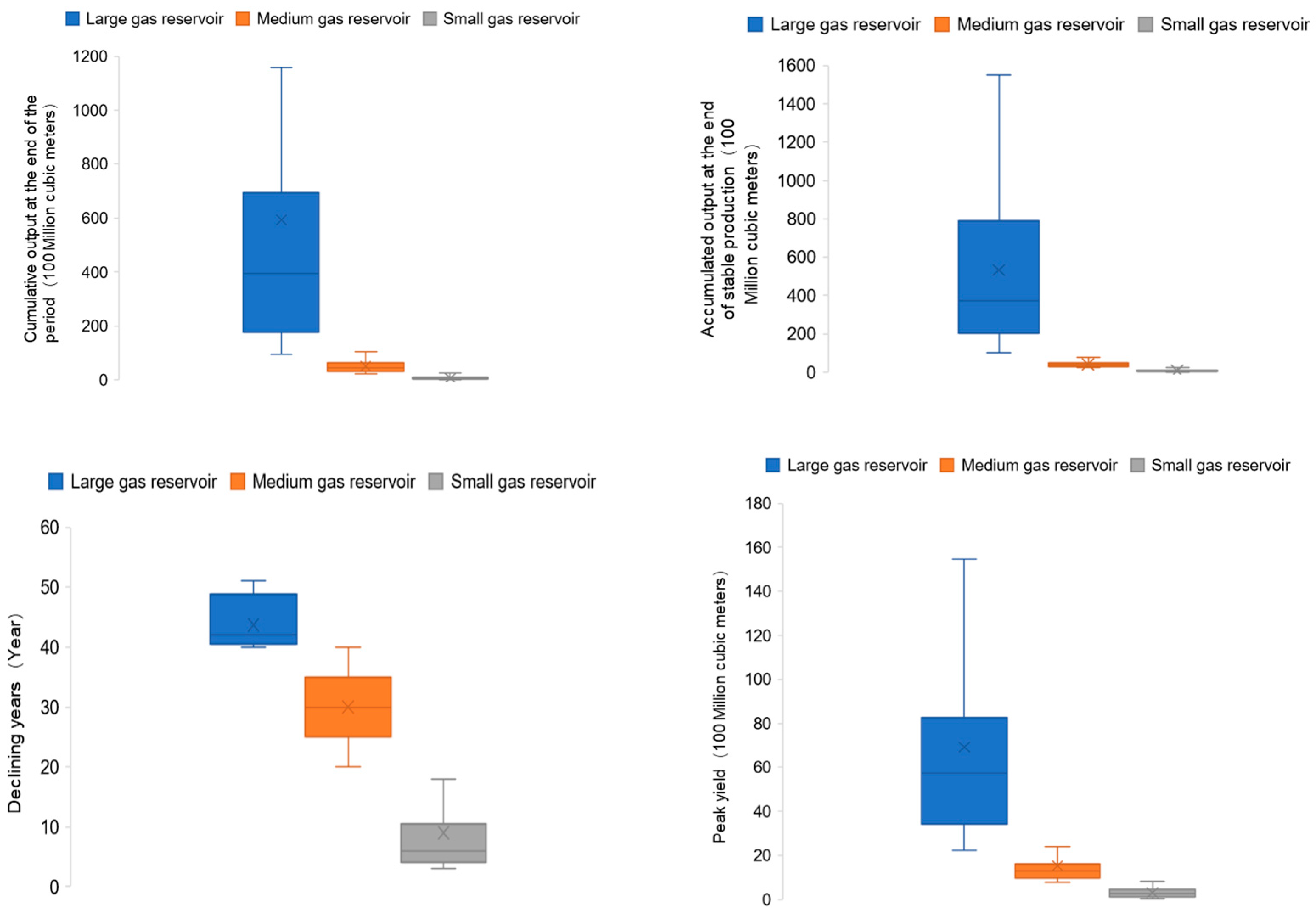
3.5. Feature Importance Selection

The model determines the importance of features based on the degree of influence of features on target variables in model training. In general, the more the feature explains the target variable, the more important it will be. The feature importance ranking generated by the LightGBM model indicates that the most important variables are the following four: Cumulative output at the end of the period, Accumulated output at the end of stable production, Peak yield, and Declining years. Other variables have a relatively minor impact on the prediction results of LightGBM. Therefore, in this experiment, it was decided to remove the variables with less impact and continue training using the selected four feature variables (Figure 7).

The overall prediction capability and classification accuracy of each model determine the quality of the predictions. Therefore, it is necessary to reevaluate the accuracy, precision, and F1 scores for different categories of tight reservoirs after removing the remaining 12 features. After feature selection, the LightGBM model achieved an overall prediction accuracy of 92%, with improved precision, recall rates, and F1 scores for different categories.

4. Discussion of Results

To better guide the actual production development of tight gas reservoirs, it is important to use data mining techniques to clarify the production characteristics of different reserves types of tight gas reservoirs. In this paper, the initial global dataset of tight gas reservoirs throughout their lifecycle was preprocessed, features were engineered, and the dataset was divided. The cleaned data was then used to train and predict using three ensemble models: Random Forest, CatBoost, and LightGBM. The best hyperparameters were found using five-fold cross-validation and grid search tuning. The performance of the three models was evaluated, and it was found that the LightGBM model had the highest accuracy, with good overall performance in terms of F1 scores for different types. This model exhibited the best predictive ability.

Therefore, the LightGBM model is used for feature importance analysis, and the model predicts that Cumulative output at the end of the period, Accumulated output at the end of stable production, Peak yield, and Declining years are the four indicators that have the best prediction effect on different categories of tight reservoirs. Shang Yongtao et al. [31] proposed a classification method for tight gas wells based on the XGBoost algorithm. The study identified the main influencing factors for gas well classification as production allocation, original formation pressure, effective thickness, porosity, and unobstructed flow rate. The researchers also conducted gas well classification in the Zimi gas field. Jia Yanran et al. [32] proposed a static-dynamic combined classification and evaluation method for low-permeability tight gas wells based on orthogonal matrix thinking. They ultimately obtained the combined static-dynamic classification results of gas wells and elucidated the relationship between reservoir properties and actual production for low-permeability tight gas wells. By comparing three models, this study proposes that the LightGBM model has the best predictive effect on tight gas reservoirs of different sizes. It also predicts the main production characteristics that affect different reserves of tight gas reservoirs. This allows for the establishment of rules for determining production characteristics that match the size of the tight gas reservoir. By analyzing the relationship between production characteristics and reserves of global tight gas reservoirs, it is possible to evaluate the production potential of different reservoirs. This can guide the rational allocation of development and production resources.

The development characteristic indicators of the LightGBM model after feature selection are analyzed (Figure 8). Cumulative_output_at_the_end_of_the_period for global tight gas reservoirs is concentrated between 0.1 and 115.8 billion cubic meters, 0.1 and 2.5 billion cubic meters for small-sized reservoirs, 2.5 and 10 billion cubic meters for medium-sized reservoirs, and 10 and 115.8 billion cubic meters for large-sized reservoirs. Accumulated_output_at_the_end_of_stable_production at the end of the period ranges from 0.2 to 154.9 billion cubic meters for global tight gas reservoirs, 0.2 to 2.4 billion cubic meters for small-sized reservoirs, 2.4 to 7.9 billion cubic meters for medium-sized reservoirs, and 7.9 to 154.9 billion cubic meters for large-sized reservoirs. Declining_years for global tight gas reservoirs ranges from 3 to 51 years, for small-scale tight gas reservoirs it ranges from 3 to 20 years, for medium-scale tight gas reservoirs it ranges from 20 to 40 years, and for large-scale tight gas reservoirs it ranges from 40 to 51 years. Peak_yield of global tight gas reservoirs ranges from 0.005 to 13.8 billion cubic meters. For small-scale tight gas reservoirs, it ranges from 0.005 to 0.8 billion cubic meters. For medium-scale tight gas reservoirs, it ranges from 0.8 to 2.3 billion cubic meters, and for large-scale tight gas reservoirs, it ranges from 2.3 to 13.8 billion cubic meters. Therefore, the development characteristics of different reserve-sized tight gas reservoirs are clarified, and a production characteristic judgment rule matching the reserve size of tight gas reservoirs is established (

Table 5. Development characteristics of tight gas reservoirs with different reserves.

Type	Decision Rule
Small gas reservoir	0.1 ≤ Cumulative_output_at_the_end_of_the_period ≤ 2.5 billion cubic meters, 0.2 ≤ Accumulated_output_at_the_end_of_stable_production ≤ 2.4 billion cubic meters, 0.005 ≤ Peak_yield ≤ 0.8 billion cubic meters, 3 ≤ Declining_years ≤ 20 years
Medium gas reservoir	2.5 ≤ Cumulative_output_at_the_end_of_the_period ≤ 10 billion cubic meters, 2.4 ≤ Accumulated_output_at_the_end_of_stable_production ≤ 7.9 billion cubic meters, 0.8 ≤ Peak_yield ≤ 2.3 billion cubic meters, 20 ≤ Declining_years ≤ 40 years
Large gas reservoir	10 ≤ Cumulative_output_at_the_end_of_the_period ≤ 115.8 billion cubic meters, 7.9 ≤ Accumulated_output_at_the_end_of_stable_production ≤ 154.9 billion cubic meters, 2.3 ≤ Peak_yield ≤ 13.8 billion cubic meters, 40 ≤ Declining_years ≤ 51 years

). This will provide possible references for the formulation of development technology policies, the development of reasonable production strategies, and the evaluation of production potential in the production development of tight gas reservoirs.

5. Case Verification

To validate the accuracy of the decision rules and production characteristics of the LightGBM model, an instance analysis was conducted on 26 tight gas reservoirs that were not involved in the decision analysis. The static indicators of the reservoirs were verified according to the model rules. The validation results indicate that this method has high accuracy and strong practicality, making it capable of accurately determining the development characteristics of tight gas reservoirs with different reserve sizes.

This paper only shows the characteristic values of four tight gas reservoirs that are not involved in decision-making analysis. Taking Loma la Lata Area gas reservoir as an example, Cumulative output at the end of the period is 78.009 billion square meters between 10 billion and 115.8 billion square meters, and Accumulated output at the end of stable production is 45.567 billion square meters between 7.9 billion and 154.9 billion square meters. The peak production is 12.347 billion cubic meters between 2.3 billion and 13.8 billion cubic meters, and the decline life is 40 years between 40 and 51 years. Therefore, the Loma la Lata Area gas reservoir is a large tight gas reservoir with more than 30 billion cubic meters of recoverable reserves. Similarly, the parameter ranges of other tight gas reservoirs are determined, and the results show that Travis Peak Tight gas ALT TX belongs to medium-sized tight gas reservoirs, while Aknazar and Churchie Area belong to small tight gas reservoirs (

Table 6. Development characteristics of typical tight gas reservoirs with different reserves.

Tight Gas Reservoir	Loma La Lata Area	Travis Peak Tight Gas ALT TX	Aknazar	Churchie Area
Cumulative output at the end of the period (100 million square meters)	780.09	52.70	11.46	1.19
Accumulated output at the end of stable production (100 million square meters)	455.67	30.43	14.65	2.43
Peak yield (100 million square meters)	123.47	12.19	5.06	0.67
Declining years (Years)	40	33	6	7
Recoverable reserves (100 million square meters)	3117.71	192.53	42.32	18.52
True type	Large gas reservoir	Medium gas reservoir	Small gas reservoir	Small gas reservoir

).

6. Conclusions

The production characteristics of reservoirs are one of the important aspects in the study of reservoir development. The production variation of reservoirs of different sizes differs. In order to better guide the production and development as well as strategy formulation of tight gas reservoirs, it is necessary to utilize data mining techniques to determine the production characteristics of different types of tight gas reservoirs. Analyzing the production characteristics patterns of tight gas reservoirs globally is of great significance for the study of development characteristics of tight gas reservoirs.

In this paper, global tight gas reservoirs are classified into three categories based on their recoverable reserves. Sixteen production features are extracted from the entire life cycle of the reservoirs. Feature engineering and data preprocessing are performed, and the Random Forest, LightGBM, and CatBoost algorithms are trained separately. The best-performing model is selected for feature importance analysis. This process establishes rules for determining production features that match the size of the tight gas reservoir, providing new ideas and methods for the development and research of tight gas reservoirs. In their study on classification methods for low-permeability tight gas wells, Jia Yanran et al. [32] used reservoir physical parameters and production dynamic indicators to classify wells based on various indicators, with rich and practical characteristic parameters. Yuan Binglong et al. [33] selected multiple relevant evaluation parameters for the classification evaluation of offshore low-permeability gas reservoirs. Based on the research findings of this paper, future improvements will be made to further enhance the selection of production characteristic parameters of reservoirs. However, due to limited data availability, there are certain limitations in the selection process, which need further refinement in order to make the obtained production characteristics of reservoirs more practical.

(1)

By using representative models such as Random Forest, LightGBM, and CatBoost for prediction and conducting optimization and comparison, it is found that the LightGBM model has the highest accuracy and overall good F1 scores for different categories. This model exhibits the best predictive capability and is more suitable for analyzing the relationship between production characteristics and different reserve sizes of tight reservoirs.

(2)

The LightGBM model selects the top four most important feature indicators, which are Cumulative output at the end of the period, Accumulated output at the end of stable production, Peak yield, and Declining years. These indicators are used to establish production feature judgment rules that match the reserve size of tight reservoirs.

(3)

The analysis of the relationship between production characteristics and reserves in global tight gas reservoirs can provide valuable references for the formulation of development technology policies, rational production strategies, and production potential evaluation in the production and development of tight gas reservoirs. For example, by analyzing the relationship between production characteristics and reserves in global tight gas reservoirs, the production potential of different reservoirs can be assessed. This helps identify which reservoirs have higher production efficiency and sustainable production levels, thereby guiding the rational allocation of development and production resources. It also helps in formulating appropriate production strategies. Reservoirs with different reserve levels may require different development and production techniques to maximize production and economic benefits. Analyzing the relationship between production characteristics and reserves can guide the selection of suitable well pattern layouts, fracturing parameters, and production control methods, thereby maximizing the production capacity of the reservoir.

References

1. Jia, A.; Wei, Y.; Guo, Z.; Wang, G.; Meng, D.; Huang, S. Development status and prospects of tight sandstone gas in China. Nat. Gas Ind. 2022, 9, 467–476. [Google Scholar] [CrossRef]
2. Jia, A.; Yan, H.; Guo, J.; He, D.; Cheng, L.; Jia, C. Development characteristics of different types of carbonate gas reservoirs. Acta Pet. Sin. 2013, 34, 914–923. [Google Scholar]
3. Duna, P.J. Analysis on development characteristics and technical measures of condensate gas reservoir. China Pet. Petrochem. Ind. 2016, 86. [Google Scholar]
4. Xu, Z.; Fang, B. Characteristics and development strategies of volcanic gas reservoirs in the Xushen gas field. Nat. Gas Ind. 2010, 30, 1–4. [Google Scholar]
5. Luo, X.; Wang, S.; Jing, Z.; Xu, G. A Study on Triassic Shale Gas Reservoir Characteristics from Ordos Basin. In Proceedings of the 2016 5th International Conference on Measurement, Instrumentation and Automation (ICMIA 2016), Shenzhen, China, 17–18 September 2016. [Google Scholar]
6. Hui, D.; Hu, Y.; Li, T.; Peng, X.; Li, Q. A typical bottom water reservoir development characteristics and suitable development strategy enlightenment. J. Oil Gas Geol. Oil Recovery 2023, 30, 101–111. [Google Scholar] [CrossRef]
7. He, D.; Yan, H.; Yang, C.; Wei, Y.; Zhang, L.; Guo, J.; Luo, W.; Liu, X.; Hu, D.; Xia, Q.; et al. Gas reservoir characteristics and development technical countermeasures of Member 4 of Dengying Formation, Anyue Gas field. Acta Pet. Sin. 2022, 43, 977–988. [Google Scholar]
8. Chen, J. Pore structure characteristics and depletion development law of deep high-pressure carbonate gas reservoirs. Spec. Oil Gas Reserv. 2022, 29, 80–87. [Google Scholar]
9. Zhou, M.; Xiang, Y.; Zhang, W.; Zhang, N.; Zhang, Y. Development characteristics and technical countermeasures of the bio-reef gas reservoir in Changxing Formation, eastern Sichuan. Nat. Gas Explor. Dev. 2020, 43, 44–51. [Google Scholar]
10. Chen, X.; Wang, G. Comprehensive classification method of low permeability reservoir. Pet. Geol. Oilfield Dev. Daqing 2014, 33, 58–61. [Google Scholar]
11. Wang, W.; Yuan, X.; Wang, G.; Liao, R. Study on classification and production characteristics of ultra-low permeability reservoirs. Pet. Drill. Technol. 2007, 72–75. [Google Scholar]
12. Li, H.; Guo, H.; Guo, H.; Meng, Z.; Tan, F. Research on mining method of complex reservoir logging evaluation data. Acta Pet. Sin. 2009, 30, 542–549. [Google Scholar]
13. Wang, L.; Wang, Z.; Tao, G. A new reservoir classification method for tight sandstone gas reservoir. Sci. Technol. Rev. 2011, 29, 47–50. [Google Scholar]
14. Liu, Y.; Zhang, X.; Zhang, W.; Guo, W.; Kang, L.; Liu, D.; Gao, J.; Yu, R.; Sun, Y. A Review of Macroscopic Modeling for Shale Gas Production: Gas Flow Mechanisms, Multiscale Transport, and Solution Techniques. Processes 2023, 11, 2766. [Google Scholar] [CrossRef]
15. Jia, A.; Yan, H.; Guo, J.; Wei, T.; He, D. Development characteristics and experience of different types of large gas reservoirs in the world. Nat. Gas Ind. 2014, 34, 33–46. [Google Scholar]
16. Li, J.; Sheng, W.; Sheng, Z.; Yin, G.; Xia, X. Research on development and Production dynamic characteristics of classified gas reservoirs in DHXH Gas Field. Offshore Oil 2019, 39, 18–22. [Google Scholar]
17. Yan, X.; Gu, H.; Xiao, Y.; Ren, H.; Ni, J. XGBoost algorithm in the application of tight sandstone gas reservoir logging interpretation. J. Pet. Geophys. Prospect. 2019, 54, 447–455+241. [Google Scholar] [CrossRef]
18. Nie, Y.; Gao, G. Based on Random Forest “Dessert” Classification Method of Shale Gas. Reserv. Eval. Dev. 1–15. Available online: http://kns.cnki.net/kcms/detail/32.1825.te.20230221.1002.002.html (accessed on 6 April 2023).
19. Shi, G. Application prospect of data mining in petroleum exploration database. China Pet. Explor. 2009, 14, 60–64+1. [Google Scholar]
20. Cheng, Q.; Wang, X.; Wang, S.; Li, Y.; Liu, H.; Li, Z.; Sun, W. Research on a Carbon Emission Prediction Method for Oil Field Transfer Stations Based on an Improved Genetic Algorithm—The Decision Tree Algorithm. Processes 2023, 11, 2738. [Google Scholar] [CrossRef]
21. Billah, M.; Islam, A.S.; Mamoon, W.B.; Rahman, M.R. Random forest classifications for landuse mapping to assess rapid flood damage using Sentinel-1 and Sentinel-2 data. Remote Sens. Appl. Soc. Environ. 2023, 30, 100947. [Google Scholar] [CrossRef]
22. Li, H.; Cao, Z.; Wu, X.; Zhu, S.; Deng, J.; Zhang, S. Prediction Method of Formation Fracture Pressure Based on LightGBM Algorithm and Its Application. Chin. Test 1–9. Available online: http://kns.cnki.net/kcms/detail/51.1714.TB.20230111.1033.001.html (accessed on 7 April 2023).
23. Wu, Y.-h. Optimization of LightGBM-XGBoost Power Load Forecasting Based on Genetic Algorithm. Sci. Technol. Innov. 2023, 71–75. [Google Scholar]
24. Xing, C.; Xu, J. LightGBM Mixture Model in the Diagnosis of Breast Cancer. Comput. Eng. Appl. 1–10. Available online: http://kns.cnki.net/kcms/detail/11.2127.TP.20230228.1116.020.html (accessed on 7 April 2023).
25. Li, H.; Tan, Q.; Zhu, S.; Deng, J.; Yan, K. Pore pressure prediction Method based on CatBoost algorithm and its application in wellbore stability analysis. China Saf. Prod. Sci. Technol. 2023, 19, 136–142. [Google Scholar]
26. Bai, G.; Zheng, L. Distribution characteristics of large gas fields in the world. Nat. Gas Geosci. 2007, 90, 161–167. [Google Scholar]
27. Jin, Z. Structure and distribution of large and medium-sized oil and gas fields in China. Xinjiang Pet. Geol. 2008, 385–388. [Google Scholar]
28. Zou, C.; Guo, J.; Jia, A.; Wei, Y.; Yan, H.; Jia, C.; Tang, H. Connotation of scientific development of large gas fields in China. Nat. Gas Ind. 2020, 7, 533–546. [Google Scholar]
29. Li, D.; Xiong, H.; Shi, G.; Niu, M. Data mining pretreatment based on global typical oil and gas field database. Pet. Geol. Oilfield Dev. Daqing 2016, 35, 66–70. [Google Scholar]
30. Li, D.; Shi, G. Optimization of common data mining algorithms in oil and gas exploration and development. Acta Pet. Sin. 2018, 39, 240–246. [Google Scholar]
31. Shang, Y.; Zhai, S.; Lin, X.; Li, X.; Li, H.; Feng, Q. Dynamic and Dynamic Integration Classification Model of Low Permeability Tight Gas Well Based on XGBoost Algorithm. Spec. Reserv. 1–12. Available online: http://kns.cnki.net/kcms/detail/21.1357.TE.20230607.1001.002.html (accessed on 13 October 2023).
32. Jia, Y.; Shi, J.; Li, X.; Chen, H.; Fang, J. Research on classification and evaluation method of low permeability tight gas Wells: A case study of Changqingzizhou gas field. Geol. Explor. 2021, 57, 647–655. [Google Scholar]
33. Yuan, B.; Ye, Q.; Zhang, L.; Chen, Z.; Lei, M. Classification method of offshore low permeability gas reservoir based on multiple evaluation parameters. J. Southwest Pet. Univ. Nat. Sci. Ed. 2020, 42, 111–118. [Google Scholar]
Figure 1. Schematic diagram of random forest generation process.
Processes 11 03159 g001
Figure 2. Schematic diagram of Leaf-wise generation process (The green nodes represent the leaf nodes with the largest split gain per cycle. Black nodes indicate other leaf nodes).
Processes 11 03159 g002
Figure 3. Dataset training modeling: schematic diagram of gradient lifting algorithm.
Processes 11 03159 g003
Figure 4. Eigenmatrix heat map.
Processes 11 03159 g004
Figure 5. Confusion matrix of the three models. (a) Random Forest, (b) LightGBM, (c) CatBoost.
Processes 11 03159 g005
Figure 6. Comparison of accuracy and F1 scores of the three models. (a) Accuracy, (b) F1 scores.
Processes 11 03159 g006
Figure 7. Importance of LightGBM model features.
Processes 11 03159 g007
Figure 8. Analysis of development characteristics of tight gas reservoirs with different reserves.
Processes 11 03159 g008