Degassing Dissolved Oxygen through Bubbling: The Contribution and Control of Vapor Bubbles

Abstract

An innovative yet sustainable approach for industrial deaeration is proposed, with demonstrated results and analyses, to contribute to finding solutions to improve energy efficiency in this field. Vacuum bubbling deaeration, sharing the same working principles of solubility control and the mass diffusion through vapor (or steam) with conventional thermal deaeration processes, works, however, at lower vacuum pressures. It neither resorts to heating nor requires any third-party materials such as membranes or gases, achieving orders of magnitude of reduction in the expected energy consumption in a simple and concrete way. In this study, the mechanisms of vapor bubble generation and retention were discussed by employing a vacuum bubbling model based on the experimental apparatus at Kongju National University, which uses a venturi-nozzle bubbler. The four parameters influencing vapor bubble generation and retention were identified as vessel pressure $p_1$, nozzle depth $\Delta h$, nozzle performance $p_4-p_3$, and water temperature $T_w$. A series of deaeration experiments using the present approach for a tap water sample of 360~400 L were conducted under four different conditions to investigate the effects of the water temperature, vessel pressure, and bubbler nozzle depth. Final dissolved oxygen (DO) concentrations close to zero could be achieved with a vessel pressure of $p_1=1 \mathrm{kPa},$with different bubbling times to reach a zero mg/L reading of DO concentration (case 2 and 3), which demonstrates the vital roles of the vapor bubble generation condition of ($p_{sat}-p_3)$ and retention condition of ($p_4-p_{sat})$ in achieving the lowest DO concentration. Analysis of the test results, based on the discrete-bubble model with the measured DO concentrations and degassing rates, showed promising results in reproducing the experimental data. Though the potential of vacuum bubbling deaeration is demonstrated, for the first time, to its full extent, further research efforts are encouraged in many areas, including more case-specific validation test cases with optimum operating conditions along with the study of more detailed modeling for performance prediction, including energy analysis.

1. Introduction

Dissolved gas in liquids and its removal have long been issues of interest for diverse applications from “artificial gills” [1,2,3,4] to deaeration processes in the energy [5,6], food and beverage [7,8], and semi-conductor manufacturing industries, etc. The required level of deaeration varies depending on the application field, while the highest levels of degassing are required in the energy industry [9] and semiconductor manufacturing processes. The heated pressure degassing process is most commonly used in energy applications [5] where the feed water is routinely heated. The overall system is complex and large-scale and uses considerable energy for deaeration through a condition-sensitive process. The feed water undergoes heating, evaporation, and condensation before the water is stripped using a portion of the steam produced in a separate boiler. In this process, spraying or tray structures are used to achieve better phase separation. Therefore, the traditional degassing process has high energy costs, high initial equipment costs, a complex system structure, and is operationally complicated. However, pressure deaerators are still widely used because they can achieve low dissolved O₂ concentrations on a large scale [9]. Membrane deaerators have gained popularity as an alternative to pressure deaerators and are currently applied in many processes [10]. Conventional methods generally require high temperature and pressure. Recently, the interest in low-energy processes and improved process efficiency to lower energy consumption has increased, and alternative technologies using vacuum technology are being introduced to mitigate the need for high pressure [11,12,13,14,15,16,17,18,19]. Other than the vacuum membrane system [20], vacuum deaeration systems still rely on a solubility limit with an extended surface area realized through either static packing materials [21,22] or dynamic rotating discs [23], but any processes that actively utilize vapor bubble diffusion under room conditions, which is the original contribution of the present study, have not been identified. Current commercially available deaerators can achieve DO concentrations of 0.5 to 0.005 mg/L, based on the literature data summarized in

Table 1. State-of-the-art deaerator performance criteria.

Application	Required DO Level (mg/L)	Method	Source (s)
Boiler feed water	≤0.005	Pressure deaerator	U.S. DOE * [9]
Food industry	≤0.01	Packing w/gas	Bucher Unipektin [21]
Beverage	≤0.01	Vac. Packing w/o gas	Corosys [19]
District heating	≤0.2	Vac. Evap. w/fillers	Eurowater [22]
Lab and pilot equipment	≤0.5	Vac. Disc. and spray	OMVE ** [23]

* U.S. DOE: The United States Department of Energy (DOE). ** OMVE: OMVE Lab and Pilot Equipment.

. As shown in Table 1, the DO concentrations vary according to the application fields and associated mechanisms. Note that boiler feed-water applications require the lowest DO concentrations where deaeration is achieved using thermal pressure deaerators. This process is based on the solubility of the gas and diffusion through steam sparging as the basic physical principles. Note also that the proposed vacuum bubbling deaeration relies on the same working principles, but works at a lower pressure and without the need for excessive heating. It should be emphasized here that mass diffusion is much more favorable with vapor bubbles under vacuum than with hot steam sparged at a higher pressure, because the partial pressure of O₂ inside the vapor bubble should be orders of magnitude less than that of hot steam. In short, it is proposed herein that vapor bubbles under vacuum conditions have a much higher degassing potential than hot steam bubbles from steam sparging.

Lower pressure operations have not received much attention thus far, mainly because of the difficulty in achieving the desired vacuum conditions in real-life situations. However, due to recent advances in technology, such as semiconductor manufacturing processes, different vacuum levels are being extensively used. As indicated in

Table 2. Degrees of vacuum and their pressure boundaries [24].

	Pressure Boundaries (mbar)	Pressure Boundaries (Pa)
Low vacuum (LV)	$1000–1$	${10}^5–{10}^2$
Medium vacuum (MV)	1–${10}^{-3}$	${10}^2–{10}^{-1}$
High vacuum (HV)	${10}^{-3}–{10}^{-9}$	${10}^{-1}–{10}^{-7}$
Ultra-high vacuum (UHV)	${10}^{-9}–{10}^{-12}$	${10}^{-7}–{10}^{-10}$
Extreme vacuum (EV)	<${10}^{-12}$	<${10}^{-10}$

, vacuum levels of interest for deaeration, around 1 kPa, are categorized as low vacuum and are considered achievable.

Based on the reviews so far, degassing experiments had been conducted at different vacuum levels [25,26], which revealed the role of hydrostatic pressure and the temperature, as well as that of vessel pressure, on the achievable degassing level. In this study, the potential of vacuum bubbling was evaluated for deaeration applications via analyses of the test conditions. For this purpose, a vacuum deaeration model is proposed based on a proprietary experimental apparatus for vacuum bubbling. Four important parameters affecting vapor bubble generation and retention are delineated, namely, the water temperature $(T_w$), vessel pressure $(p_1$), nozzle performance $(p_4-p_3$), and the nozzle depth $\left(\Delta h\right)$, which are directly related to the vapor generation condition $p_{sat}-p_3$ and vapor retention condition $p_4-p_{sat}$. This study presents experimental results that reflect the effect of the vapor bubble retention conditions on vacuum bubbling at two different nozzle depths, that is, 30 cm and 20 cm from the water surface. By monitoring the volume of the extracted gas captured, as well as the DO concentration over time, important performance metrics such as the lowest DO concentration, time, and energy consumption are determined. The experimental results are discussed in relation to the analysis of a model developed based on the measured extracted gas volume data.

2. Materials and Methods

2.1. Background Physics

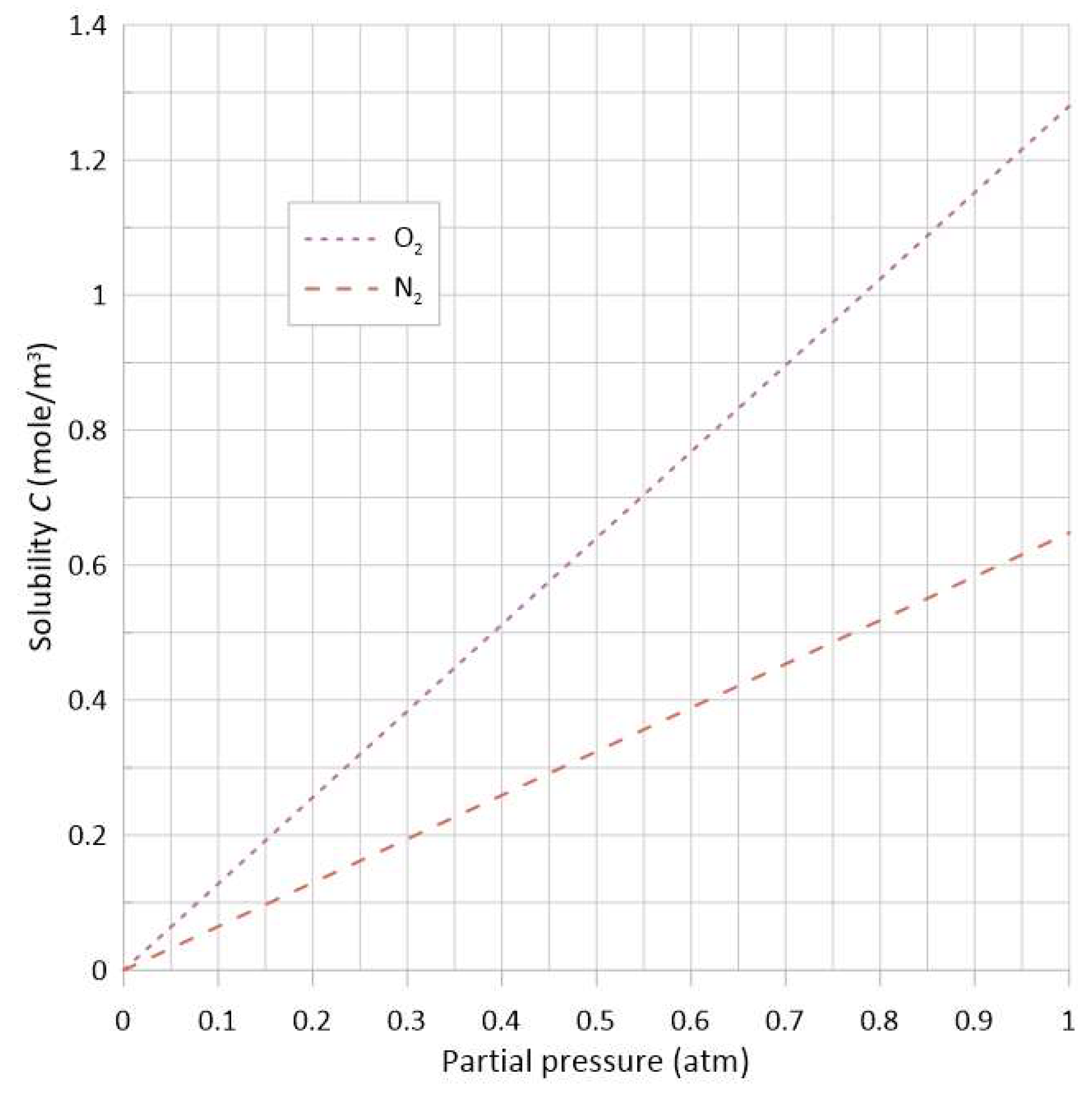
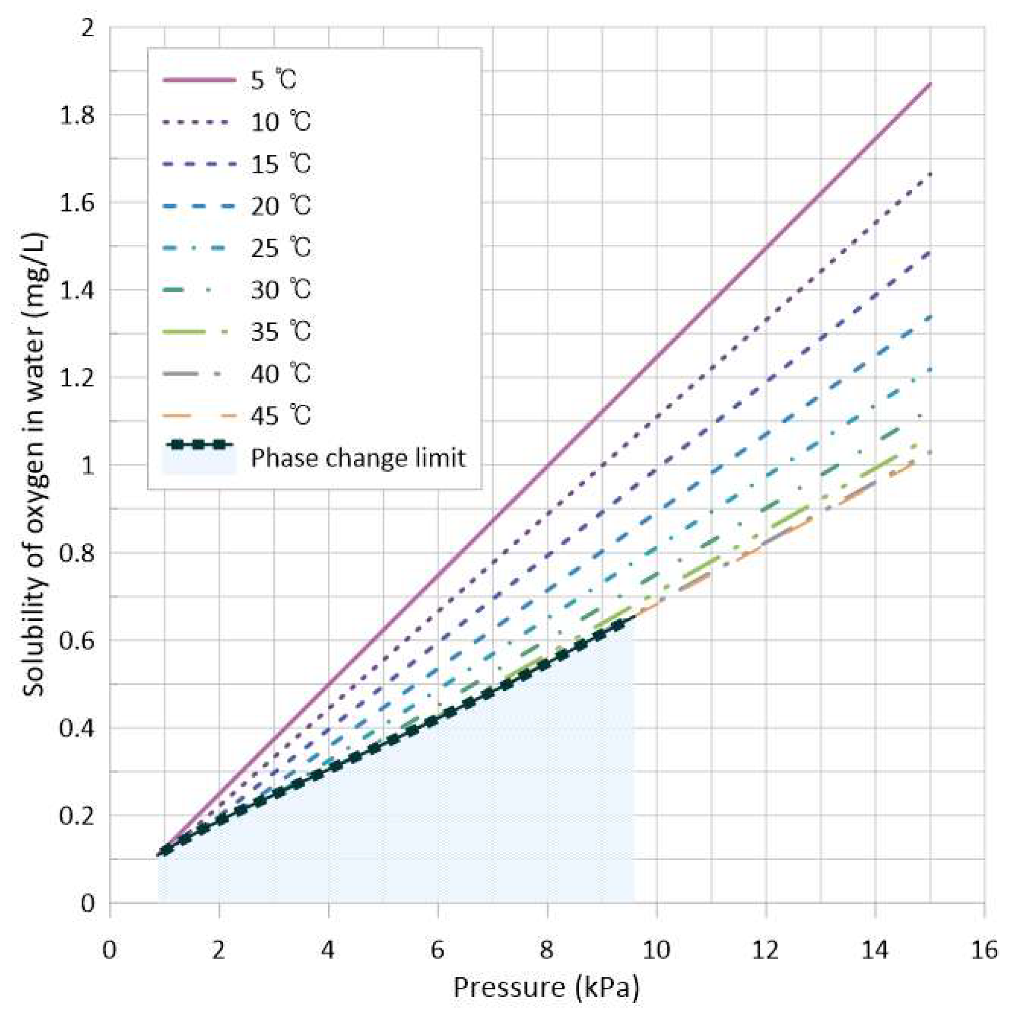
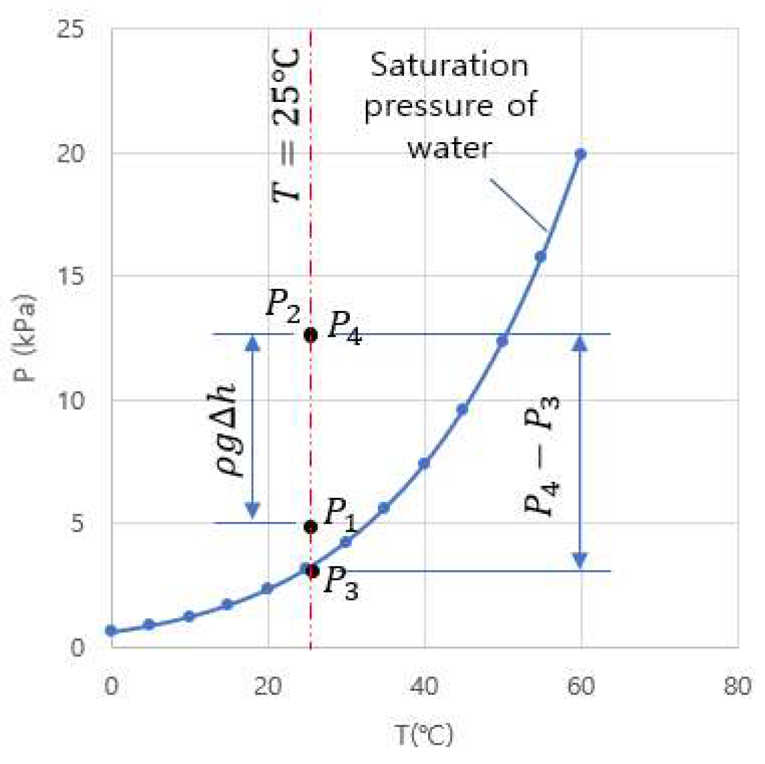
2.1.1. Solubility Behavior with Respect to Temperature and Pressure

Solubility decreases with temperature, as illustrated in Figure 1, and is proportional to the partial pressure of the solute gas, which is known as Henry’s solubility law.

$$C_{s,i}= H_i{P}_i .$$

(1)

Here, $C_{s,i}$ is the solubility (mol/L∙atm), $H_i$ is Henry’s constant, and $P_i$ is the partial pressure of a specific gas (atm). Figure 2 illustrates the variation of the solubility of O₂ and N₂ in water at 25 °C, according to Henry’s law, with the constant values shown in

Table 3. Henry’s solubility constants for O₂ and N₂ in water at 25 °C [28].

Species	Unit	Henry’s Constant H
O2	mol/(L·atm)	$1.28\times {10}^{-3}$
N2		$6.48\times {10}^{-4}$

. Note that heating can lower the solubility of a gas in a liquid, thereby eliminating the dissolved gas species [6]; however, the same effect can be achieved using depressurization, with less energy.

Once the solubility decreases, regardless of the trigger (heating or vacuum), the portion of supersaturated solutes that are in an unstable state can escape from the liquid, in the form of bubbles, without much difficulty. However, manipulating the solubility by controlling the pressure has a lower limit for application, because a phase change is induced at low pressures near the saturated vapor pressure, below which the solvent (water), at least theoretically, may no longer exist in a stable liquid state.

A solvent such as water undergoes a phase change according to its thermodynamic state, which is represented by a phase-change diagram. Henry’s law deals with the saturated solubility of a solute in a liquid solvent; however, if the pressure is so low that it falls below the saturated vapor pressure of the liquid solvent, the phase of the solvent may change from liquid to vapor, and Henry’s solubility law may no longer be applicable. Figure 3 illustrates Henry’s law for the solubility of O₂ in water at different temperatures, with the lower limit set by the saturated vapor pressure of water at each temperature [29]. Henry’s law is only effective if the solvent remains in a liquid state. Once the liquid solvent is vaporized under vacuum, vapor bubbles may be generated as a gas mixture composed of water vapor and the dissolved gas at the point of vaporization.

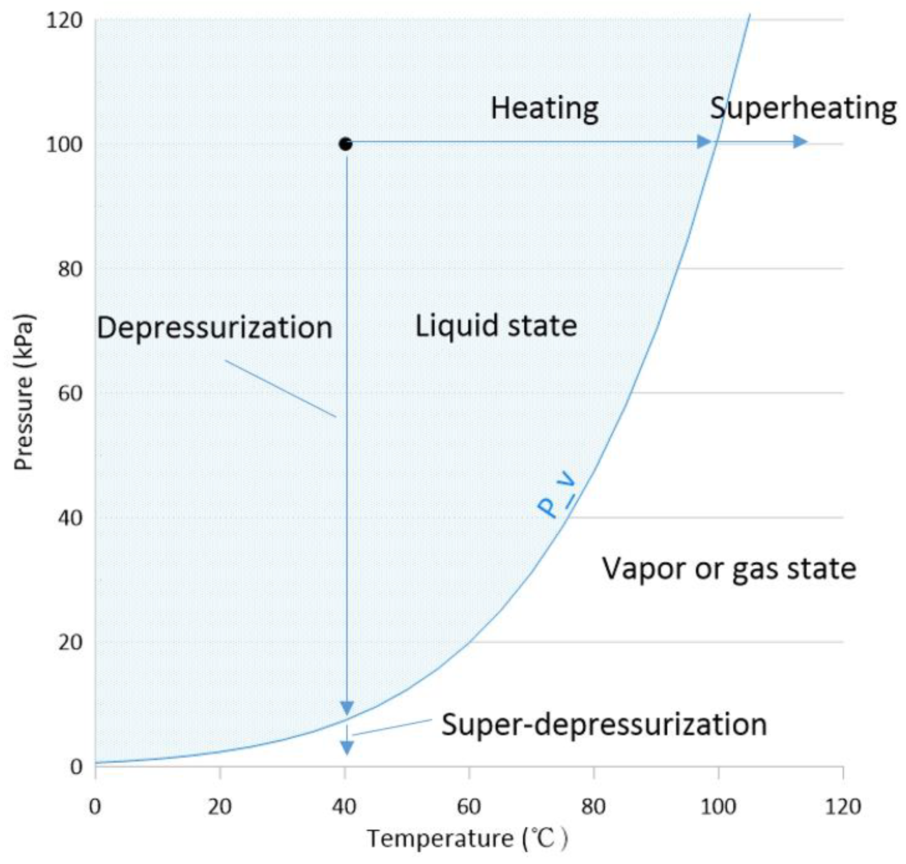
2.1.2. Bubble Generation—Tension vs. Superheating

Vapor bubbles are cavitation bubbles that may appear when the local pressure decreases below the vapor pressure of the liquid, which is a function of temperature. Figure 4 presents a phase-change diagram based on the saturated vapor pressure of water.

During heating, vaporization occurs at the superheated locations of a surface after reaching the saturation temperature, whereas under a vacuum, vaporization may occur if the local pressure falls below the saturated vapor pressure of the liquid. One important aspect of the two different paths for vaporization (heating vs. depressurization) lies in the fact that while heating is a direct input of energy into the water system, depressurization is not. Depressurization affects only the surrounding conditions and not the system itself, resulting in a significant difference in energy use. For example, let us consider the energy required to reach the vaporization state from the assumed room conditions ($T_1=$ 25 °C, $p_1=$ 101.3 kPa) via heating to a state of $T_2=$ 100 °C, $p_2=$ 101.3 kPa, or depressurization or vacuuming to a state of $T_2^{\prime }=$ 25 °C, $p_2^{\prime }=$ 3.17 kPa. Assuming there is $m=$ 400 kg of water in the vessel with $V_1=$ 21.1 L of headspace, which corresponds to one of the present experimental conditions described later, in the case of heating, the heat energy of $Q=mc\left(T_2-T_1\right)=400 \mathrm{kg}\times 4.18 \mathrm{kJ}/\left(\mathrm{kg}·°\mathrm{C}\right)\times \left(100-25\right)°\mathrm{C}=125,400 \mathrm{kJ}=34.8 \mathrm{kWh}$ is required before the phase change is initiated. Here, the specific heat of water at 25 °C is assumed to be $4.18 \mathrm{kJ}/\left(\mathrm{kg}·°\mathrm{C}\right).$ In comparison, in the case of the depressurization of air under an assumed constant-temperature process, the work required to decompress the headspace becomes $W=p_1{V}_1{{\displaystyle \int }}_{V_1}^{V_2^{\prime }}\frac{dV}{V}=p_1{V}_{1}ln\left(\frac{V_2^{\prime }}{V_1}\right)$. Noting that $V_2^{\prime }=V_1\frac{p_1}{p_2^{\prime }}=21.1\times \frac{101.3}{3.17}=674.3$L, $W=p_1{V}_{1}ln\left(\frac{V_2^{\prime }}{V_1}\right)=101.3\times 21.1\times ln\left(\frac{674.3}{21.1}\right)=7.4 \mathrm{kJ}=0.00206 \mathrm{kWh}$. The ratio of the work energy required for process 1 to change to 2′, with respect to the heat energy required for process 1 to change to 2, is $\frac{7.4}{125,400}=0.00006,$which is negligible. Although this estimation is based on ideal thermodynamic relationships, the data indicate that the burden of the heating energy can be almost completely eliminated by utilizing vacuuming as an alternative process.

When one considers a phase-change phenomenon, such as the generation of vapor bubbles, uniform equilibrium conditions are usually difficult to achieve. Instead, local and transient phenomena are important. Brennen [30], one of the pioneers in vapor bubble studies, describes:

“If a pure liquid at a subcooled state is depressurized at constant temperature, and pressure is reduced below that of the saturated vapor pressure without significant nucleation sites, the depressurization may lead to continuation of the state down the theoretical isotherm to a point where the pressure is below the saturated vapor pressure. The pressure difference between this local pressure and the saturated vapor pressure is the magnitude of the tension.” Brennen also notes that “the necessary condition for vapor bubble generation is related to the extent of tension and the duration.”

Brennen’s description of material behavior near the phase change is significant. First, if insufficient energy is supplied to induce a phase change from the liquid state to the vapor state, no phase change may occur. The energy for vaporization, $h_{fg}$, is a well-known property of liquids such as water and is only a function of temperature. This suggests that in a metastable region near the phase-change line, the extent of vaporization will depend on the amount of energy input, regardless of the energy form, either heat or pressure. Second, once the material is in a metastable region and is in a certain phase, this phase will remain unchanged; otherwise, energy input is required to induce the phase change, which means that once the liquid is vaporized and the thermodynamic condition is maintained, the vapor will remain in its current phase.

2.1.3. Diffusion Potential of Steam and Vapor Bubbles

Based on the assumption that dry air is composed of 79.1% N₂ and 20.9% O₂, if vapor bubbles are created instantly by decompressing the inside of liquid water that is initially in phase equilibrium with atmospheric pressure, the concentrations of O₂ and N₂ in the liquid are $C_{O_2}=8.3 \mathrm{mg}/\mathrm{L}=\frac{8.3 \times {10}^{-3} \mathrm{g} \times 1\frac{\mathrm{mol}}{32}\mathrm{g}}{1 \mathrm{L} \times {10}^{-3 {\mathrm{m}}^3/\mathrm{L}}}=0.259 \mathrm{mol}/{\mathrm{m}}^3$ and $C_{N_2}=13.9 \mathrm{mg}/\mathrm{L}=\frac{13.9 \times {10}^{-3}\mathrm{g} \times 1\frac{\mathrm{mol}}{28}\mathrm{g}}{1 \mathrm{L} \times {10}^{-3{ \mathrm{m}}^3/\mathrm{L}}}=0.496 \mathrm{mol}/{\mathrm{m}}^3,$ respectively. If the pressure of this solution is reduced, for example, to 1 kPa, which is lower than the saturated vapor pressure, the saturated solubility becomes undefinable according to Henry’s law, because the solvent (water) would no longer exist in the liquid phase. In this case, the volume of each component originally contained in 1 L of water is ascertained to calculate the concentration of each constituent inside the bubble, instead of using the saturation solubility at the interface.

$$V_{O_2}=\frac{m_{O_2}{R}_{O_2}T}{p}=\frac{8.3\times {10}^{-6 }\mathrm{kg}\times 0.2598 \mathrm{kJ}/\mathrm{kg}·\mathrm{K}\times 298.15 \mathrm{K}}{1 \mathrm{kPa}}=0.00064{ \mathrm{m}}^3$$

$$\begin{gathered} V_{N_2}=\frac{m_{N_2}{R}_{N_2}T}{p}=\frac{13.9\times {10}^{-6} kg\times 0.2968 \mathrm{kJ}/\mathrm{kg}·\mathrm{K}\times 298.15 \mathrm{K}}{1 \mathrm{kPa}} \\ =0.00123 {\mathrm{m}}^3 \end{gathered}$$

$$V_{vap}=\frac{m_{vap}{R}_{vap}T}{p}=\frac{0.997 \mathrm{kg}\times 0.4615\frac{\mathrm{kJ}}{\mathrm{kg}}·\mathrm{K}\times 298.15 \mathrm{K}}{1 \mathrm{kPa}}=137.183{ \mathrm{m}}^3$$

From this, the volume fraction of O₂ inside the bubble becomes $y_{O_2}=\frac{V_{O_2}}{V_{O_2}+V_{N_2}+V_{vap}}=\frac{0.00064}{0.00064+0.00123+137.183}=4.6\times {10}^{-6}$.

The result of this calculation suggests that the volume fraction of O₂ inside the evaporated water is very low, close to zero, even though no pre-degassing was involved, and similar results hold for water evaporated at high temperatures under atmospheric pressure conditions. However, it should be emphasized that even though the volume fractions in the two cases were similar, the partial pressure levels of the dissolved gas, which are the working variables in the diffusion process [31], were significantly lower under vacuum. Noting that this low concentration originates from the volume expansion of water to the vapor state, the concentration difference is maintained throughout the deaeration process, which provides a strong drive for mass diffusion and accounts for why, compared to other methods, vapor-bubbling deaeration is expected to provide the lowest dissolved O₂ concentration.

2.1.4. Bubble Diffusion

Modeling was attempted as part of the present study, based on a discrete-bubble model [32,33] developed for aeration applications. Unlike aeration practices, where air is supplied to a specific bubbling aeration system at a certain rate, the bubbling parameters in the case of deaeration, including the bubble generation rate, initial bubble size, and composition, should be determined separately, possibly through experiments. With these in mind, the discrete bubble model for aeration was extended to deaeration applications.

Herein, the following assumptions are made: (1) the initial bubble size can be determined from its Sauter mean diameter (SMD), and the rate of bubble formation can be determined from the experiments, (2) the mass transfer of O₂ and N₂ occurs with no bubble coalescence, (3) the temperature of the water and air is constant and equal, and (4) the mass transfer through the free surface of the water at the top is negligible.

The mass-transfer flux (subscript i for either O₂ and N₂) across the surface of a bubble is

$$J_i=K_L\left(C_{si}-C_i\right) \left({\mathrm{molm}}^{-2}{s}^{-1}\right),$$

(2)

$\mathrm{where} K_L$ is the liquid-side mass transfer coefficient, $C_s$ is the equilibrium concentration at the gas/water interface, and $C$ is the bulk aqueous-phase concentration. The gas-side mass transfer resistance was assumed to be negligible. The equilibrium concentration was determined using Henry’s law, Equation (1). Substituting the expressions from Equation (1) into Equation (2) yields

$$J_i=K_L\left(H_i{P}_i-C_i\right) \left({\mathrm{molm}}^{-2}{s}^{-1}\right).$$

(3)

The rate of mass transfer for a single bubble is obtained by multiplying the surface area of a bubble of radius $r$ by

$$\frac{d{m}_i}{dt}=-K_L\left(H_i{P}_i-C_i\right)4\pi r^2 \left({\mathrm{mols}}^{-1}\right)$$

(4)

The vertical location of a bubble is determined by the bubble-rise velocity $v_b$, and any induced vertical water velocity $v$, as follows:

$$\frac{dz}{dt}=v+v_b\left({\mathrm{ms}}^{-1}\right)$$

(5)

where z denotes the vertically upward direction. The induced velocity $v$, may be lower than the bubble-rise velocity. A unique feature of this discrete bubble model is that instead of performing time integration on the mass diffusion and vertical location separately, the model combines Equations (4) and (5) to obtain the mass of the gaseous species transferred per bubble per unit height of the tank as follows:

$$\frac{d{m}_i}{dz}=-K_L\left(H_i{P}_i-C_i\right)\frac{4\pi r^2}{v_b} \left({\mathrm{molm}}^{-1}\right)$$

(6)

through which the time t is no longer involved as a variable. The initial number flux of bubbles, N, was estimated based on the initial bubble volume, $V_0$, and the actual volumetric gas flow rate at the diffuser, $Q_0$:

$$N=\frac{Q_0}{V_o}\left(s^{-1}\right)$$

(7)

The molar flow rate of the gas, M, was obtained by multiplying Equation (6) by N:

$$\frac{d{M}_i}{dz}=-K_L\left(H_i{P}_i-C_i\right)\frac{4\pi r^{2}N}{v_b} \left({\mathrm{molm}}^{-1}{s}^{-1}\right)$$

(8)

When a bubble rises, the concentration of the bulk aqueous phase is assumed to remain constant. Equation (8) is integrated numerically for each O₂ and N₂ species to obtain the change in the molar flow rate when the bubble is in contact with water during its rise.

Table 4. Correlations used in the discrete bubble model (Henry’s constants, bubble-rise velocity, and the liquid-side mass transfer coefficient) [33].

Property or Variable Name	Correlation Equation	Range
H (${\mathrm{molm}}^3{\mathrm{bar}}^{-1}$)	$H_{O_2}=2.125-5.021\times {10}^{-2}{T}^2+5.77\times {10}^{-4}{T}^2$ (T in °C)	Not available
	$H_{N_2}=1.042-2.450\times {10}^{-2}{T}^2+3.171\times {10}^{-4}{T}^2$ (T in °C)
$K_L$ (${\mathrm{ms}}^{-1})$	$K_L=0.6r$	$\mathrm{r}<6.67\times {10}^{-4}$ m
	$K_L=4\times {10}^{-4}$	$\mathrm{r}\ge 6.67\times {10}^{-4}$ m
$v_{b }$ (${\mathrm{ms}}^{-1})$	$v_b=4474r^{1.357}$	$\mathrm{r}<7\times {10}^{-4}$ m
	$v_b=0.23$	$7\times {10}^{-4}\le \mathrm{r}<5.1\times {10}^{-3}$ m
	$v_b=4.202r^{0.547}$	$\mathrm{r}\ge 5.1\times {10}^{-3}$ m

summarizes the correlations used in the discrete bubble model.

Using these relationships and the change in the bubble radius, both the bubble-rise velocity and mass transfer coefficient were recalculated as the bubble traveled upwards. Once the bubbles reached the surface, the overall changes in the molar flow rate of the gas (both O₂ and N₂) were used to calculate the evolving concentration of the bulk aqueous phase as a function of time. The initial molar flow rates of the gaseous O₂ and N₂ were

$$m_0=\frac{Y_0{P}_{std}{Q}_{std}}{R{T}_{std}} \left({\mathrm{mols}}^{-1}\right)$$

(9)

where $Y_0$ is the initial mole fraction of the gas, $P_{std}$ is the standard pressure, $Q_{std}$ is the gas flow rate at standard temperature and pressure (0 °C and 1 bar), $R$ is the ideal gas constant, and $T_{std}$ is the standard temperature.

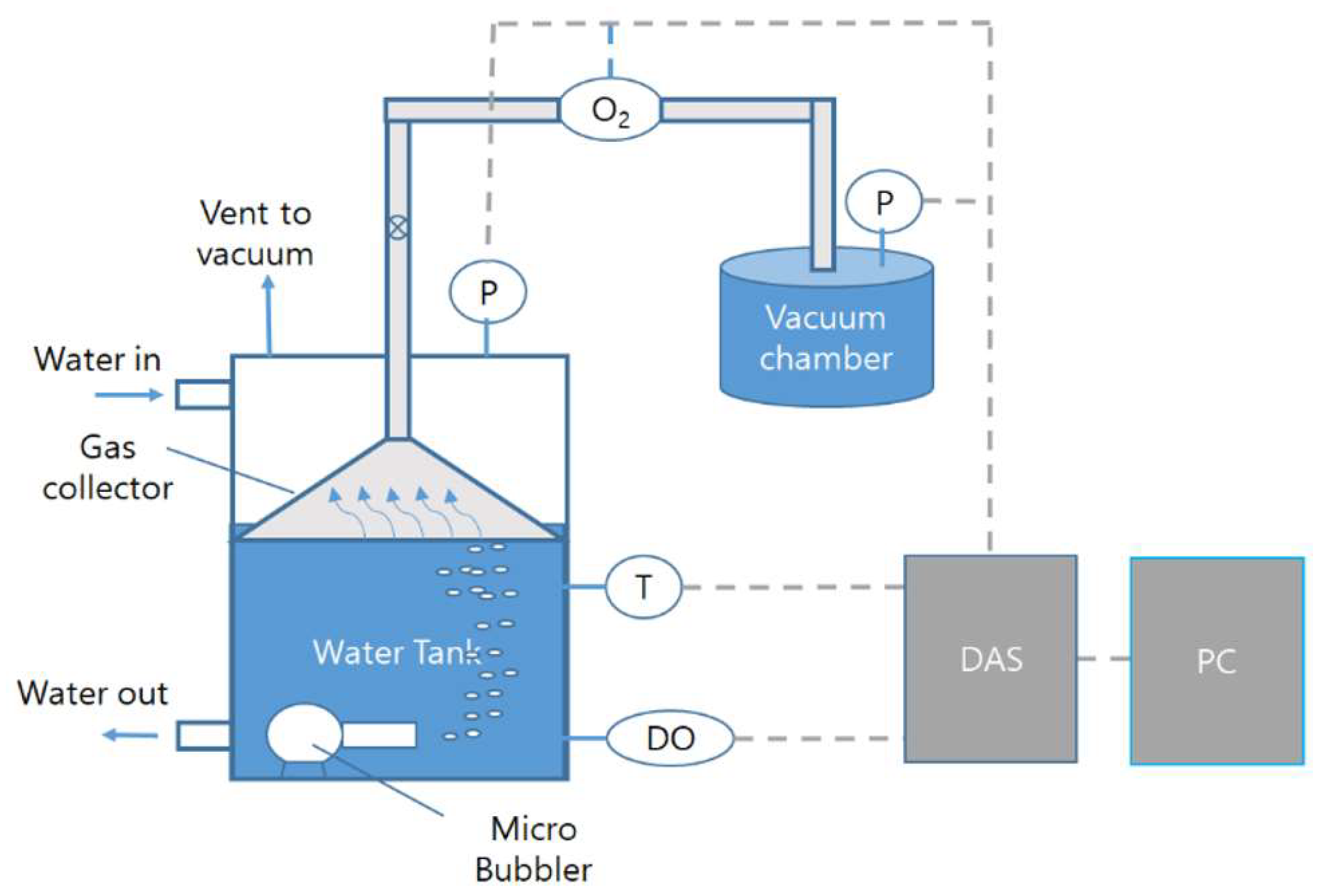
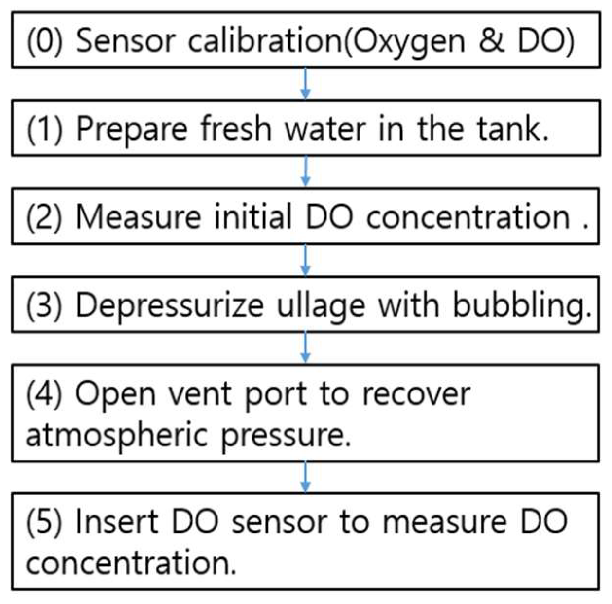
2.2. Experimental Setup and Test Methods

Figure 5 presents an illustration of the test apparatus used in this study, which was composed of a sealed water vessel with a depressurization system, a Venturi-type microbubble generator [26], a gas collector hood, and a data acquisition system (Yokogawa DA-100, 30 Ch.; Japan). The water vessel, 0.65 m (L) × 0.65 m (W) × 1.0 m (H) in size, was equipped with two large viewing windows, as shown in Figure 6, through which the actual phenomena occurring during the test could be visually monitored. A gas-collector hood was installed inside the tank to capture the extracted dissolved gas. For the vessel pressure and water temperature measurements, a digital pressure transducer (Ulfa Technology, SDT series B760H, $\pm 760 \mathrm{mmHg}, \mathrm{res}. 1 \mathrm{mmHg}$, Republic of Korea) and K-type thermocouples were used.

In the present study, cavitation bubbling was achieved by lowering the local pressure at the nozzle throat, through which flow was induced by a 12 V DC water pump (Daehwa Electric, DPW69-12, 12 V DC, 69 lpm; Busan, Republic of Korea), along with depressurization of the ullage space using a vacuum pump (Kodivac Ltd., oil-sealed rotary pump, GHP-340K, 0.75 kW; Gyeongsan, Republic of Korea). A Venturi-type bubble-generator nozzle [26] was installed at a certain height above the bottom of the vessel. The gas extracted via bubbling was collected under a gas-collector hood inside the tank, as shown in Figure 5 and Figure 6. Once a sufficient volume of gas was captured, degassing was stopped and the tank pressure was recovered to atmospheric pressure for measurement of the DO (Mettler-Toledo InPro 6950(i) Oxygen Measurement Sensor with M300 Multi-parameter Transmitter, 6–50,000 ppm, $\pm 5 \mathrm{ppm}$; Switzerland); this sequence comprised one degassing session. The collected gas level was measured using a scale attached to the slanted surface of the gas collector and was converted to the corresponding volume using a pre-constructed calibration curve [25]. The test procedure is illustrated in Figure 7.

2.3. Vacuum Bubbling Model and Analysis of Test Condition

2.3.1. Vacuum Bubbling Model

To better understand the vapor bubble generation conditions, a theoretical operation model for vacuum vapor bubble generation (Figure 8) is presented herein, based on the present experimental model.

The vessel was filled with tap water, and a vent for depressurization and gas discharge was connected to a vacuum device at the top of the container. A bubbler nozzle connected to a submersible pump that was installed horizontally at a depth ∆h in the water. For the sake of discussion, room condition is denoted by the subscript 0; the ullage space by the subscript 1; and the nozzle inlet, throat, and downstream conditions by subscripts 2, 3, and 4, respectively. The room temperature (T₀) and water temperature (T_w) were assumed to be the same.

Vacuum bubbling consists of two steps. In the first step, the entire ullage space is depressurized to a pressure close to the saturated vapor pressure, followed by additional local depressurization (through the bubbler nozzle) to below the saturated vapor pressure, at which vapor bubbles are generated. A more detailed view of the thermodynamic state using the abovementioned model (Figure 8) reveals how the conditions vary depending on the operating conditions. For the purpose of this discussion, the baseline operation conditions are defined as follows:

-

water temperature $T_w=25 °\mathrm{C}$;

-

nozzle depth ∆h = 0.8 m;

-

ullage pressure $p_1=5 \mathrm{kPa}$;

-

fixed flow rate through the nozzle (driven by a pump using DC power of 20 W).

One of the two steps in vacuum bubbling is to reduce the pressure inside the vessel $p_1$using a vacuum pump, and the other is to reduce the local pressure using the flow induced by the pump. When the flow is induced by the pump, the pressure at each part of the nozzle is represented by $p_2$, $p_3$, and $p_4$ which correspond to the nozzle inlet, throat, and downstream, respectively, as shown in Figure 9. Note that $p_3$, the minimum local pressure, occurs at the nozzle throat and is related to the condition for vapor bubble generation $p_{sat}-p_3$, whereas $p_4$, the nozzle downstream pressure, is related to the vapor bubble retention condition $p_4-p_{sat}$. Note also that $p_4$ depends on the depth of the nozzle (∆h), such that $p_4=p_1+\rho g\Delta h$ due to the effect of the hydrostatic pressure contribution at that depth. Out of the figure, one can identify four important performance variables that directly affect the conditions for the generation and retention of vapor bubbles. These four performance variables are the decompression level $p_1$, nozzle depth $\Delta h$, water temperature T_w, and nozzle performance $p_4-p_3$ as illustrated in Figure 9. Vapor bubble generation appears to be governed by the extent of tension, $p_{sat}-p_3$, whereas vapor bubble retention is governed by the downstream condition$p_4-p_{sat}$ and these two values are determined by the combinations of those four physical variables.

2.3.2. Analysis of Test Conditions

The tests were designed and conducted to confirm the effects of the variables, starting with the baseline operation conditions; the test conditions are summarized in

Table 5. Test conditions and analysis.

Case	${\mathit{p}}_1$ (kPa)	$\Delta \mathit{h}$ (m)	${\mathit{p}}_4$ (kPa)	${\mathit{p}}_4-{\mathit{p}}_3$ (kPa)	${\mathit{p}}_3$ (kPa)	${\mathit{T}}_{\mathit{w}}$ (°C)	${\mathit{p}}_{\mathit{s}\mathit{a}\mathit{t}}$ (kPa)	${\mathit{p}}_{\mathit{s}\mathit{a}\mathit{t}}-{\mathit{p}}_3$ (kPa)	${\mathit{p}}_4-{\mathit{p}}_{\mathit{s}\mathit{a}\mathit{t}}$ (kPa)
0 (Baseline)	$5$	0.8	12.82	9.65 1	3.17	25	3.17	0	9.65
1	5	0.8	12.82	9.65 1	3.17	35	5.63	2.46	7.19
2	1	0.3	3.93	9.65 1	(−5.72)	18.6	2.16	(7.88)	1.77
3	1	0.2	2.96	9.65 1	(−6.69)	22	2.67	(9.36)	0.29

¹ Estimated for the nozzle used with a fixed nominal pump power input of 23.4 W.

. The nozzle performance$\left(p_4-p_3\right)$ was estimated for a pump input power of 23.4 W for all test cases. According to the test conditions’ analyses, the vapor generation condition $\left(p_{sat}-p_3\right)$ was marginal (near zero) with the baseline conditions (case 0) and increased to a maximum potential in case 3. The values in parentheses reflect non-physical values (negative pressure and related values) because once vaporization occurs, the pressure may no longer decrease. Therefore, these values should be considered, instead, to be driving potential and not to be real pressure values. The nozzle downstream condition $(p_4-p_{sat}),$ which represents the deviation of the nozzle downstream pressure from the saturated vapor pressure, is related to the vapor retention. Among the test cases, case 3 afforded the best retention, with the lowest deviation of 0.29 kPa (Table 5). When the vessel pressure, $p_1$ was maintained at 5 kPa, as in cases 0 and 1, the nozzle downstream pressure $p_4$ reached 12.82 kPa due to the hydrostatic contribution of nozzle depth, resulting in significant deviation from the phase change pressure of $3.17 \mathrm{kPa}$ at the specified temperature of 25 °C, whereas in cases 2 and 3, the vessel pressure was maintained at 1 kPa, which provided favorable bubble generation conditions, but with different nozzle downstream conditions depending on the nozzle depths. Here, $p_1=1 \mathrm{kPa}$ was lower than the saturated vapor pressure of water at the corresponding temperatures of 18.6 °C and 22 °C. The test conditions of case 2 and 3 differ only in the nozzle depth, resulting in different nozzle downstream conditions ($p_4-p_{sat}).$ The pressure difference $p_4-p_3$, was estimated to be 9.65 kPa with a flow rate of 13.42 lpm based on an assumed pump efficiency of 50% and the minor losses due to the inlet, contraction, and diffusion through the Venturi-nozzle [26].

3. Results

The time variations of the DO concentration were measured for the four test cases, including the baseline condition (case 0), and the degassing rates were also measured for cases 2 and 3, in which significant evidence of vapor bubbling was expected based on the test condition analysis, as shown in Table 5. The total electricity usage is also provided for further discussion of energy-saving issues. The presented results are a subset of the experimental data at different conditions and double checked for repeatability by the author.

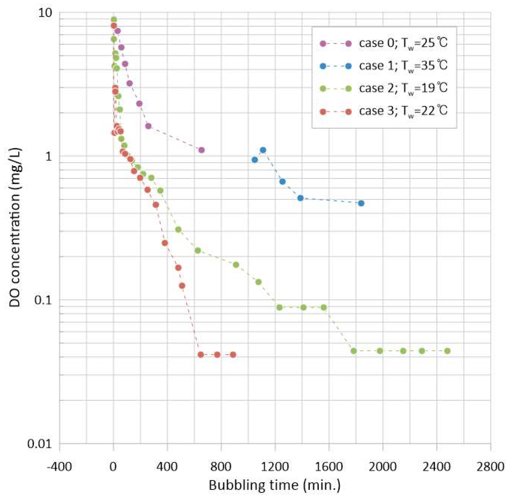
3.1. Variation of DO Concentration (Minimum DO and Time)

Figure 10 shows the measured DO concentration (mg/L) with respect to the bubbling time. When the vacuum levels were not low enough to generate enough vapor bubbles, $p_1=5 \mathrm{kPa}$ (cases 0 and 1), the conditions for vapor generation ($p_{sat}-p_3$) were marginal, that is, at 0 and 2.46 kPa, respectively (Table 5). The resulting minimum DO levels were found to be ~1.1 mg/L for case 0 and 0.47 mg/L for case 1 with a higher water temperature of 35 °C. The difference between the two cases arises from the temperature difference being elevated by 10 °C. However, no further decrease in DO concentration was detected. However, when the vessel pressure was lowered to 1 kPa (cases 2 and 3), with lower values of $\Delta h$, the tension for vapor bubble generation ($p_{sat}-p_3)$ significantly increased, with different levels of vapor bubble retention conditions of $p_4-p_3=1.77 \mathrm{kPa} \left(\mathrm{case} 2\right) \mathrm{and} 0.29 \mathrm{kPa} \left(\mathrm{case} 3\right)$, respectively. In both cases, the DO concentration reached 0 mg/L, but at different rates. Note that the resolution of the measurement unit (Mettler-Toledo M300 instrument with polarographic DO sensor) was limited to 0.1%-atm, which corresponds to 0.04 mg/L. Based on these results, the aim of achieving a sufficiently low DO concentration with vacuum-bubbling deaeration seems to have been met.

A lower DO concentration was achieved in test case 1, where the temperature was higher (35 °C) than in case 0, because the saturated vapor pressure increased by 2.46 kPa (from 3.17 kPa to 5.63 kPa) in the former (Table 5), resulting in more favorable conditions for vapor bubble generation as the tension increased from 0 to 2.46 kPa, which also led to more favorable conditions for bubble retention. However, these two cases appear to provide poor conditions for the generation and retention of vapor bubbles. As shown in Figure 10, a minimum DO concentration of 0 mg/L was achieved for both cases 2 and 3 after 2551 and 998 min of bubbling time, respectively. The zero (0) data values are not shown in the figure because of the use of a logarithmic scale for representing the concentration. The rate of decrease in the DO concentration differs under these two conditions (cases 2 and 3) mainly because of the nozzle downstream condition, where the generated vapor bubbles are eventually exposed. Note that in case 3, the pressure deviates less from the phase-change condition, $p_4-p_{sat}=0.29 \mathrm{kPa}$, compared to case 2, $p_4-p_{sat}=1.77 \mathrm{kPa}$. The chances of remaining in a metastable state should be higher when the deviation of the pressure from the saturated vapor pressure is smaller.

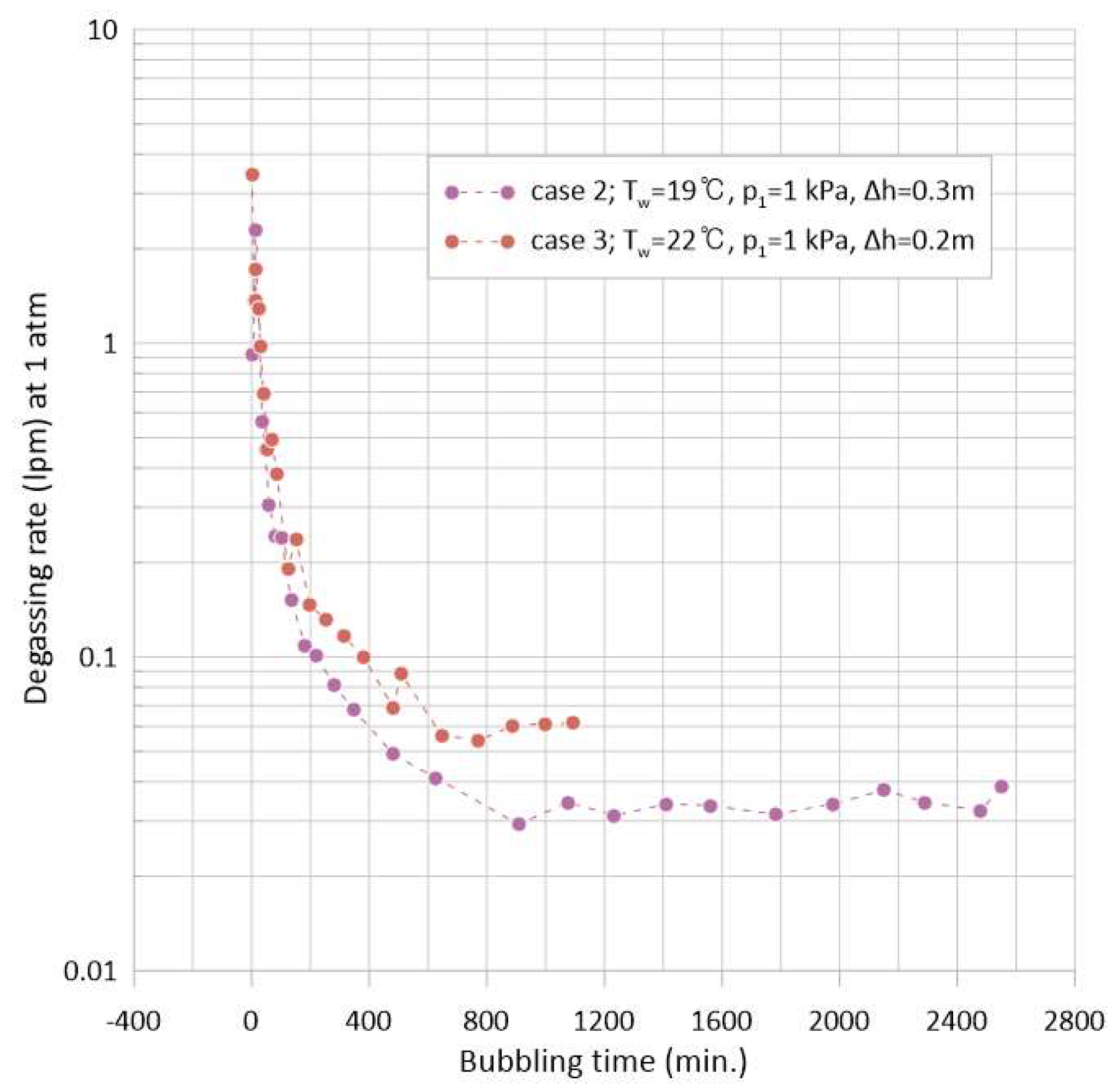
3.2. Degassing Rate and the Rate Model

Figure 11 shows the measured degassing rates for cases 2 and 3 at a vessel pressure $p_1$ of 1 kPa. The degassing rates were determined by reading the scale attached to the slanted side of the gas collector hood, as shown in Figure 6 and Figure 7, and converting the value through a pre-established calibration curve. Degassing started with a high flow rate, with a maximum of 3.4 lpm in case 3, followed by a rapid exponential decrease, but did not converge to zero in either case. The degassing rate eventually approached an almost constant value depending on the conditions of each case. This is a unique finding, as the pressure is below the saturated vapor pressure compared to the findings in the cases of $p_1>p_{sat}$, in which no bubbles were generated after a certain period. From this observation, it is deduced that once most of the supersaturated solutes are removed via degassing, water vapor and the remaining portion of the dissolved gas may vaporize. Referring to the data for $p_4-p_{sat}$ in Table 5, it appears that a higher tension at the throat and lower deviation from the phase-change condition are more favorable for vapor bubble generation and retention, resulting in higher degassing rates, as shown in Figure 11. Average vapor bubble degassing rates of 0.034 and 0.061 lpm were obtained for cases 2 and 3, respectively, based on the observed gas volumes from each session. Note that the pressure acting on the captured gas is higher than $p_1$, as indicated by the lower water surface level in the collector hood, and is estimated to be 2.3 kPa. Under more favorable conditions, the vapor bubble degassing rate in case 3 was 80% higher than that in case 2.

Figure 12 shows typical images of the vacuum bubbling process during the initial (Figure 12a) and final (Figure 12b) stages. In the initial stage, massive bubbles exited the bubbler nozzle, with a rapid decrease in the amount of degassing, whereas a limited amount of bubbles were steadily generated after a certain period. The natural deduction from this observation is that the constant degassing rates in the latter part of the degassing process are only due to vapor bubbles, whereas the initial transient values include the portion of supersaturated solutes in the water and the constant rates from vapor bubbles. The analysis is conducted based on this observation.

3.3. Energy Consumption for Degassing

The electricity consumption was monitored during the deaeration experiments. The DC water pump with a maximum output of 100 W for the bubbler was run during the entire bubbling time, with a constant nominal rate of 20 W (2.73 Amp × 7.3 VDC). The electricity usage could be estimated by multiplying the nominal rate by the total bubbling time. The vacuum pump (a 0.75 kW oil-sealed rotary pump) was operated intermittently and the energy consumption from the start of the vacuum application to the end of the deaeration experiments was measured using a power meter. The total bubbling time and the electricity consumption required to arrive at a reading of 0 DO %-atm are summarized in

Table 6. Energy consumption for vacuum bubbling deaeration experiments.

Test Case	Water Vol. (m3)	Total Bubbling Time (min.)	Epump (kWh)	Evac·p (kWh)	Etotal (kWh)
Case 2	0.40	2551	0.847	0.822	1.669
Case 3	0.36	998	0.331	0.467	0.798

and Figure 13 for cases 2 and 3. The data in Table 6 reveal that the right choice of operating conditions is critical for securing the desired deaeration performance in terms of not only the minimum DO concentration, but also of total bubbling time (Figure 13a), and the electrical energy consumption (Figure 13b). A simple comparison of cases 2 and 3, for which the vessel pressure was the same, demonstrates that the time required to reach 0 DO %-atm in case 3 was less than half the time required in case 2, resulting in 60% less bubbling time (Figure 13a) and 52% less energy use (Figure 13b) than the former case, which is significant. Considering the water volumes used for each case, the normalized energy use is 4.17 kWh/m³ and 2.22 kWh/m³ for cases 2 and 3, respectively. Further efforts are required to determine the optimum operating conditions. Care should be paid when these data are used for comparison to ensure a fair judgement.

4. Discussion

Figure 11 shows that bubble generation during the degassing process may be considered to be divided into two apparent modes: in the first mode, the bubble generation declines exponentially, whereas in the second mode, the bubbling rate is almost constant. This is an interesting phenomenon that needs to be studied further, because knowing the gas composition and supply rates is a prerequisite for degassing simulations. It is hypothesized, regarding the composition of the bubbles, that the initially formed bubbles are characterized by supersaturated solutes that were dissolved in the solvent, whereas the bubbles generated in the latter part are characterized by vapor bubbles. Based on this, an approximate model for the composition of the bubbles is presented as follows:

(1)

The two gas sources, supersaturated solutes and water vapor, contributed simultaneously, with different contribution fractions.

(2)

The degassing rate of the vapor is assumed to be constant and determinable (from experiments).

(3)

The extracted gas is composed of vapor bubbles, as determined in (2), and supersaturated solutes, which are responsible for the remaining degassing rate.

Based on the above assumptions, the initial conditions for the discrete bubble model described in Section 2.1.4 can be determined. Based on the mass balance calculation, the assumed bubble composition at the time of generation was obtained as follows:

Determination of the mass balance equation:

(1)

The total rate of the volume change for the extracted gas was determined from the experiment: $Q_N\left(t\right) \left(\mathrm{N} \mathrm{lpm}\right)$.

(2)

The total rate of the volume change for the extracted gas was interpreted as the sum of the vapor bubbles and dissolved gases (O₂ and N₂): $Q_N\left(t\right)=Q_{N,vap}\left(t\right)+Q_{N,s}\left(t\right)$

Note that $Q_{N,vap}$ (N lpm) was obtained from the experiments and the rate of the volume change of the supersaturated solutes: $Q_{N,s}=Q_N\left(t\right)-Q_{N,vap}\left(t\right)$

(3)

The initial composition of the supersaturated solutes was estimated based on the measured DO concentration or the assumed equilibrium conditions.

$$Q_{N,O_2}=Q_{N,s}\times 0.332$$

$$Q_{N,N_2}=Q_{N,s}\times 0.636$$

(4)

As time advances, $Q_N\left(t\right)$ was updated by measurements or using correlation equations, as shown in Figure 14.

$$Q_N\left(t\right)=0.2738\times t^{-0.88} (\mathrm{N}-\mathrm{lpm}) \mathrm{for} 0< \mathrm{t} <t_{phase}$$

$$Q_N\left(t\right)=0.00073 (\mathrm{N}-\mathrm{lpm}) \mathrm{for} \mathrm{t} >t_{phase}$$

In case 2, $t_{phase}$= 900 min. The degassing rates are expressed in terms of N lpm for convenience of calculation under normal conditions (0 °C and 1 atm), and the pressure at which the gas volume is measured during the degassing experiment is assumed to be 2.3 kPa, considering the lowered water level in the collector hood. The Henry’s solubility law constants for O₂ and N₂ in water used in this model are as follows:

$$H_{O_2}=2.125-5.021\times {10}^{-2}\times T+5.77\times {10}^{-4}\times T^2(\mathrm{mol}/{\mathrm{m}}^3·\mathrm{bar})$$

and

$$H_{N_2}=1.042-2.450\times {10}^{-2}\times T+3.17\times {10}^{-4}\times T^2(\mathrm{mol}/{\mathrm{m}}^3·\mathrm{bar})$$

Based on the above assumptions, the volume rate of change for the bubbled gas is shown in Figure 15, where the contributions of the total and individual components of the gases are given.

Before the overall deaeration analysis was conducted, the region of vapor bubble degassing was of particular interest because, in that region, after approximately 500 min of bubbling time, a clear contribution of vapor bubbles was demonstrated through the change in the DO concentration (case 2 in Figure 10). The initial bubble size could be estimated by analyzing this region. Figure 16 shows the estimated variation in the DO concentration with respect to time at a measured average degassing rate of 0.0344 L/min; the pressure is assumed to be 2.3 kPa considering the lowered water surface level inside the collector when the gas is captured.

The overall deaeration process was attempted using the most probable SMD for the vapor bubbles, which was determined to be 0.32 mm from the case 2 experiment. Figure 17 shows the analysis results for the overall deaeration process based on the discrete bubble model, with the assumption that the gas comprises a mixture of vapor and air, as shown in Figure 16, and the bubble SMD at the location of bubble generation remained the same from the beginning to the end of the deaeration process. The simulated results agree fairly well with the measured data, with only a slight overestimation of the extent of deaeration, which seems justifiable considering the stringent assumptions of a constant (mean) bubble size without any merging or coalition of bubbles. In Figure 17, the overall concentration change was characterized by three zones. In the first zone, most of the gases constituting the bubbles were dissolved gases, because of the decrease in solubility due to the pressure change. In the test results for case 2, this zone extended for up to approximately 1 h after the initiation of bubbling. During this period, the DO concentration decreased sharply to approximately 1 mg/L. In the second zone, the rate of decrease in the DO concentration was slightly more gradual. In this zone, the proportions of dissolved gas and vapor were comparable, and the DO concentration in the water decreased relatively slowly. Over time, the amount of dissolved O₂ remaining in the water was limited due to continued degassing. In the third zone, mass transfer between the vapor bubbles and the dissolved O₂ remaining in the water drives deaeration at a lower level until the end of the experiment. Note that the concentration difference between the liquid and vapor states is the result of volume expansion during the phase change, and the concentration difference or ratio remains constant throughout the process until the value approaches zero. This zone shows a lower rate of change in concentration than the previous zones, but the lowest dissolved O₂ concentration could be realized through continuous operation. The present test results and the analysis suggest that the present deaeration approach, vacuum bubbling, can realize the lowest DO level expected in industry, with identified control variables and with a methodology that can analyze and estimate the performance of the system in question.

5. Conclusions

A simple, high-performance, yet energy-efficient approach for deaeration is introduced for possible practical applications, with the expectation that this method may contribute to improving the energy efficiency of the process, which is known to be a task for the industry in attempting to pursue a sustainable future. Of the two working mechanisms of vacuum bubbling, solubility and mass diffusion through vapor bubbles, the latter, which has received less research interest to date, is discussed in detail. The major findings of this study are as follows:

• Vapor bubbles with a DO volume fraction of less than 10⁻⁶, due to the effect of volume expansion during the phase change process, are responsible for mass diffusion at the lowest DO concentration levels, close to zero.
• The conditions for the generation and retention of vapor bubbles under vacuum are explicitly delineated in this study, along with other influential variables. The tension ($p_{sat}-p_3)$ at the bubbler nozzle throat defines the vapor generation condition, while the deviation from the phase-change pressure ($p_4-p_{sat})$ downstream of the bubbler nozzle defines the condition for vapor bubble retention in the present experimental system. The effect of these factors was demonstrated through experiments (cases 2 and 3), showing that even under the same vessel pressure $p_1$= 1 kPa, the time required for a zero mg/L reading of DO concentration could be reduced by 60% depending on the nozzle depth change in the present study, which is one of the influential parameters herein.
• The total energy consumption required to complete the degassing of the water body to 0 mg/L at room temperature was measured and reported in the present study. The energy used during the experiments includes the electric power for a water pump and a vacuum pump. The minimum deaeration time for 0.36 m³ of water was found to be 998 min (case 3), with a total electricity consumption of 0.829 kWh (2.31 kWh/m³).
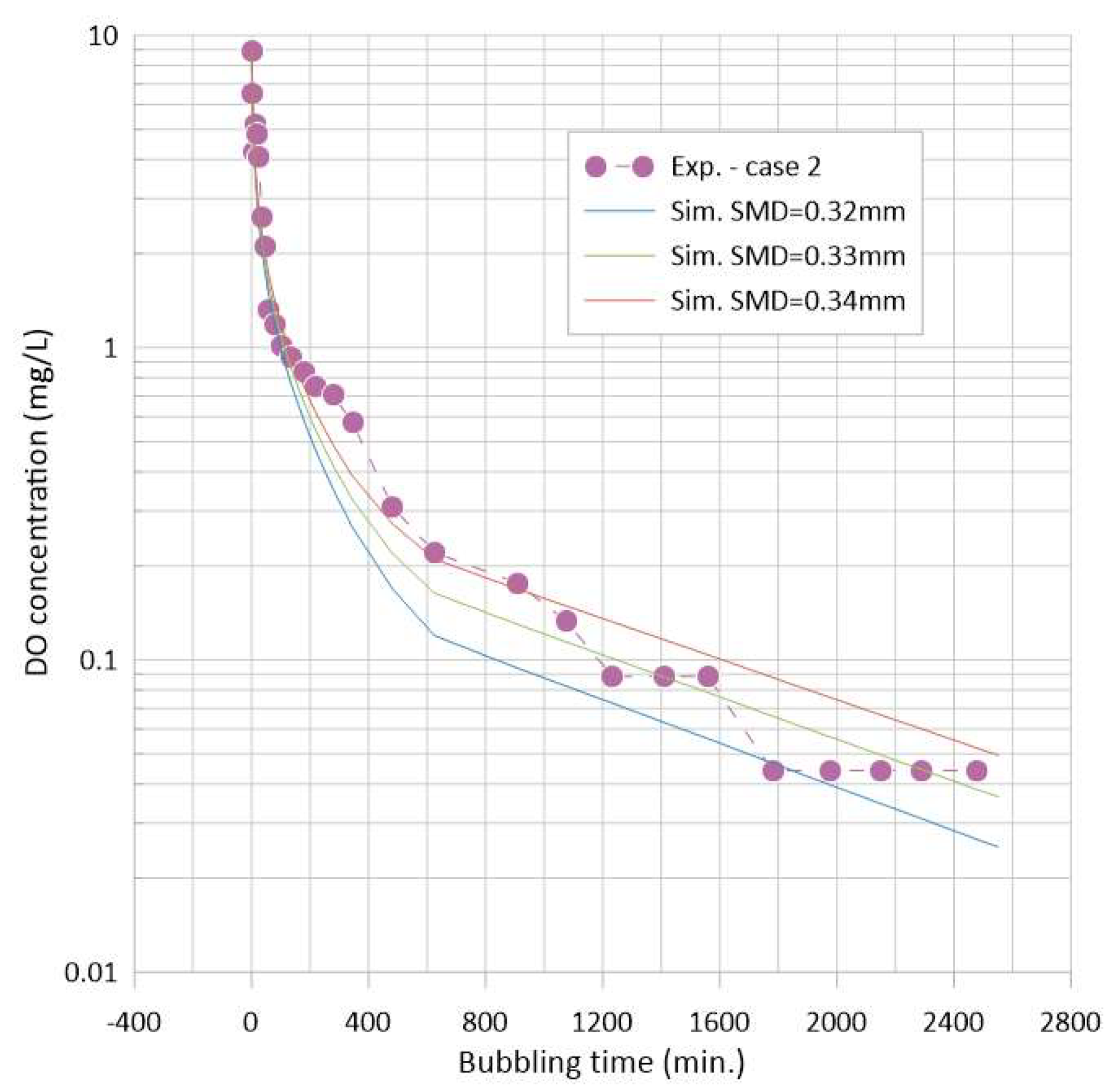
• Although case-specific, attempts were made to analyze the test results and to develop a predictive model for the present approach. Based on the estimated SMD of the initial vapor bubbles, the entire bubbling behavior could be reproduced using the discrete-bubble model with the measured degassing rate. Further efforts are encouraged for model refinement and validation.

Through the present study, it was demonstrated that deaeration down to zero mg/L DO concentration could be achieved, largely due to the contribution of vapor bubbles. Understanding the vapor bubble generation and retention conditions seems critical in achieving vapor bubbling, which provides a theoretical tool to secure the optimum operating conditions for individual applications. The energy required, though not directly compared with data from other approaches in the present study, is also compared theoretically against the heating process, but more extensive comparisons are desired for fairer estimations. The model, although case-specific, provides a concrete view of the behavior of the deaeration process. The present approach fundamentally differs from other vacuum devices that rely on solubility, including the surface controls, and can provide the minimum level of, or better than, thermal deaerators without resorting to heating and without the need for any third-party materials as membranes or gases. It is to be noted, however, the resolution for DO measurements was found to be not optimal for use in the current extreme pressures and at a low level.

References

1. Lee, J.W.; Heo, P.W.; Kim, T.S. Theoretical model and experimental validation for underwater oxygen extraction for realizing artificial gills. Sens. Actuators A Phys. 2018, 284, 103–111. [Google Scholar] [CrossRef]
2. Ieropoulos, I.; Melhuish, C.; Greenman, J. Artificial gills for robots: MFC behavior in water. Bioinsp. Biomim. 2007, 2, S83–S93. [Google Scholar] [CrossRef] [PubMed]
3. Bodner, A. Available online: http://www.likeafish.biz (accessed on 3 November 2023).
4. Kim, G.B.; Kim, S.J.; Kim, M.H.; Hong, C.U.; Kang, H.S. Development of a hollow fiber membrane module for using implantable artificial lung. J. Membr. Sci. 2009, 326, 130–136. [Google Scholar] [CrossRef]
5. Water Treatment: Aeration and Gas Stripping—TU Delft OpenCourseWare. Available online: https://ocw.tudelft.nl/wp-content/uploads/Aeration0and-gas-stripping-1.pdf (accessed on 24 December 2021).
6. Arthur, D. How Does Deaerator Work? Available online: http://watertreatmentbasics.com/how-does-deaerator-work/ (accessed on 24 December 2021).
7. Greenbank, G.R.; Wright, P.A. The deaeration of raw whole milk before heat treatment as a factor in retarding the development of the tallowy flavor in its dried product. J. Dairy Sci. 1951, 34, 815–818. [Google Scholar] [CrossRef]
8. Carlsson, H.; Jönsson, C. Separation of Air Bubbles from Milk in a Deaeration Process. 2012. Available online: https://www.researchgate.net/publication/267687974 (accessed on 3 November 2023).
9. U.S. Department of Energy. Deaerators in Industrial Steam Systems. (Brochure).; 2012. Available online: https://www.energy.gov/sites/prod/files/2014/05/f16/steam18_steam_systems.pdf (accessed on 3 November 2023).
10. 3MTM Liqui-CelTM Membrane Contactors. A High Level of Consistency and Control. Available online: https://multimedia.3m.com/mws/media/2091084O/3m-spsd-liqui-cel-general-brochure.pdf (accessed on 21 August 2023).
11. Vacuum Deaerator. Eurowater, Vacuum Deaerator|Remove Oxygen and Carbon Dioxide from Make-Up Water. Available online: https://www.eurowater.com/en/water-treatment-plants/deaeration/vacuum-deaerator (accessed on 3 November 2023).
12. Vacuum Deaeration, EWT Water Technology, Vacuum Deaeration. EWT Water Technology. Available online: https://www.ewt-wasser.de/en/product/vacuum-deaerator.html (accessed on 3 November 2023).
13. WhittierTM Vacuum Deaerators. Industrial Grade Degasification. Available online: https://www.veoliawatertechnologies.com/en/technologies/whittier-vacuum-deaerators (accessed on 21 August 2023).
14. American Water Chemicals®. Deaeration Systems. Available online: https://www.membranechemicals.com/water-treatment/deaeration-systems/ (accessed on 21 August 2023).
15. Zero Gas Vacuum Deaerator. Available online: https://www.cannonartes.com/systems-equipment/deaeration/zerogas-vacuum-deaerators/ (accessed on 21 August 2023).
16. Vacuum Deaerator (DEB). Available online: https://bachiller.com/en/vacuum-deaerator/ (accessed on 21 August 2023).
17. PerMix. PerMix Vacuum Deaerator. Available online: https://www.permixmixers.com/liquid-mixers/permix-vacuum-deaerator/ (accessed on 21 August 2023).
18. TechniBlend. Beverage Deaeration. Available online: https://www.techniblend.com/products/beverage-deaeration/ (accessed on 21 August 2023).
19. High Vacuum Water Deaeration V2WD. Available online: https://bbt.corosys.com/en/solutions/degassing/high-vacuum-water-deaeration-v2wd/ (accessed on 21 August 2023).
20. Ulfa Technology Co. Ltd. Operations Manual for Developer Degassing System (UDO-3006B-1). (In Korean). Available online: https://www.ulfatech.com/home/wp-content/uploads/pdf/UDO-3006B.pdf (accessed on 2 December 2022).
21. Bucher Unipektin. Deaerator for the Food Industry. Available online: https://www.directindustry.com/prod/bucher-unipektin-ag/product-89865-2522723.html (accessed on 2 December 2022).
22. Eurowater. Vacuum Deaerator. Available online: https://www.eurowater.com/en/water-treatment-plants/deaeration/vacuum-deaerator (accessed on 2 December 2022).
23. OMVE. Vacuum Deaerator DEA 310. Available online: https://www.directindustry.com/prod/omve-lab-pilot-equipment/product-50514-349872.html (accessed on 2 December 2022).
24. Chiggiato, P. Vacuum Technology for Superconducting Devices. In Proceedings of the CAS-CERN Accelerator School: Superconductivity for Accelerators, Erice, Italy, 24 April–4 May 2013; Bailey, R., Ed.; CERN-2014-005 (CERN, Geneva, 2014). [Google Scholar]
25. Hong, J.A.; Lee, J.S.; Jun, Y.-D. Degassing Dissolved Oxygen through Bubbles under a Vacuum Condition. In Proceedings of the 7th Thermal and Fluids Engineering Conference (TFEC), Las Vegas, NV, USA, 15–18 May 2022. [Google Scholar]
26. Jun, Y.-D. Degassing behavior of water through bubbling near a vapor pressure condition. In Proceedings of the 16th International Conference on Heat Transfer, Fluid Mechanics and Thermodynamics (HEFAT2022-ATE), Amsterdam, The Netherlands, 8–10 August 2022; pp. 277–282. [Google Scholar]
27. Engineering ToolBox. Solubility of Air in Water. 2004. Available online: https://www.engineeringtoolbox.com/air-solubility-water-d_639.html (accessed on 17 March 2022).
28. Yoo, S.H. (Ed.) Encyclopedia of Soil Science; Seoul National University Press: Seoul, Republic of Korea, 2000; pp. 443–444. ISBN 89-521-0204-5. (In Korean) [Google Scholar]
29. Klein, S. Engineering Equation Solver (EES) by F-Chart Software, Accompanying Thermodynamics an Engineering Approach, 7th Edition in SI Units; McGraw-Hill: New York, NY, USA, 2011. [Google Scholar]
30. Brennen, C.E. Cavitation and Bubble Dynamics; Oxford University Press: New York, NY, USA, 1995; pp. 16–17. [Google Scholar]
31. Incropera, F.P.; Dewitt, D.P.; Bergman, T.L.; Lavine, A.S. Fundamentals of Heat and Mass Transfer, Sixth Ed.; John Wiley & Sons: Hoboken, NJ, USA, 2007; pp. 882–884. [Google Scholar]
32. Wüest, A.; Brooks, N.H.; Imboden, D. Bubble Plume Modeling for Lake Restoration. Water Resour. Res. 1992, 28, 3235–3250. [Google Scholar] [CrossRef]
33. McGinnis, D.F.; Little, J.C. Predicting diffused-bubble oxygen transfer rate using the discrete-bubble model. Water Res. 2002, 36, 4627–4635. [Google Scholar] [CrossRef] [PubMed]
Figure 1. O2 solubility in fresh water (courtesy of The Engineering Toolbox [27]).
Processes 11 03158 g001
Figure 2. Solubility of O2 and N2 in water at 25 °C with variation of the pressure.
Processes 11 03158 g002
Figure 3. Solubility of O2 in water at different temperatures under 1 atm, with phase change limits.
Processes 11 03158 g003
Figure 4. Vapor bubble generation methods: heating vs. depressurization (vapor pressure data for water from [29]).
Processes 11 03158 g004
Figure 5. Test apparatus for degassing experiments.
Processes 11 03158 g005
Figure 6. Test apparatus showing the water tank with a gas-collector hood inside.
Processes 11 03158 g006
Figure 7. Test procedure for degassing and measurements (Steps (0) to (2) initialize the test condition, while steps (3) to (5) are repeated and define a measurement session).
Processes 11 03158 g007
Figure 8. A theoretical operation model for vacuum vapor bubble generation.
Processes 11 03158 g008
Figure 9. Model of baseline operating conditions for vacuum bubbling experiment ( Δ h = 0.8   m ).
Processes 11 03158 g009
Figure 10. Variation of measured DO concentration with bubbling time for the four different test conditions described in Table 5.
Processes 11 03158 g010
Figure 11. Degassing rates measured at 1 kPa.
Processes 11 03158 g011
Figure 12. Typical views of vacuum bubbling.
Processes 11 03158 g012
Figure 13. Time and energy consumption for different deaeration experiments.
Processes 11 03158 g013
Figure 14. Two degassing modes (phase 1: solubility-driven degassing, phase 2: vapor bubbles).
Processes 11 03158 g014
Figure 15. Assumed volume rate of change for bubbled gas and the component gases.
Processes 11 03158 g015
Figure 16. Comparison of change in DO concentration due to vapor bubbles only.
Processes 11 03158 g016
Figure 17. Comparison of DO concentration change during deaeration.
Processes 11 03158 g017