Model and Analysis of Pump-Stopping Pressure Drop with Consideration of Hydraulic Fracture Network in Tight Oil Reservoirs

Abstract

The existing pump-stopping pressure drop models for the hydraulic fracturing operation of tight oil reservoirs only consider the main hydraulic fracture and the single-phase flow of fracturing fluid. In this paper, a new pump-stopping pressure drop model for fracturing operation based on coupling calculation of the secondary fracture and oil-water two-phase flow is proposed. The physical model includes the horizontal wellbore, the fracture network and the tight oil reservoir. Through the numerical simulation and calculation, the wellbore afterflow performance, the crossflow performance between the main hydraulic fracture and the secondary fracture, the fracturing fluid leakoff and the oil-water replacement after termination of pumping are obtained. The pressure drop characteristic curve is drawn out by the bottom-hole flow pressure calculated through the numerical simulation, and a series of analyses are carried out on the calculated pressure drop curve, which is helpful to diagnose the -oil-water two-phase flow state and the fracture closure performance under the control of the fracture network after hydraulic fracturing pumping. Finally, taking a multi-stage fractured horizontal well in a tight oil reservoir in the Junggar basin, China as an example, the pump-stopping pressure drop data of each stage after hydraulic fracturing are analyzed. Through the history fitting of the pressure drop characteristic curve, the key parameters such as fracture network parameters, which include the half-length of main hydraulic fracture, the conductivity of main hydraulic fracture and the density of secondary fracture, the fracture closure pressure are obtained by inversion, thus, the hydraulic fracturing effect of fractured horizontal well in tight oil reservoirs is further quantified.

1. Introduction

The effective development of unconventional shale reservoirs benefits from large-scale hydraulic fracturing technology. The pressure drop curve after the termination of pumping in hydraulic fracturing operations reflects the closing law of underground hydraulic fracture and the law of oil-water migration. The decreasing law of bottom-hole or wellhead pressure with time after termination of pumping is related to reservoir rock mechanics characteristics, fluid characteristics and fracture parameters. The quick evaluation of the fracturing effect can be realized by analyzing and fitting the characteristics of the pressure drop curve after the termination of pumping.

In the past 40 years, scholars have completed a lot of research on the theory and analysis methods of the pressure drop model after the termination of pumping in the fracturing operation. In 1979, Nolte [1] first put forward the viewpoint that the pressure decline in the fracture closure period after fracturing reflects the fracture and its surrounding strata, and the viewpoint and method of calculating fracturing parameters by using a pressure drop curve. Based on the PKN two-dimensional fracture model, a pressure drop mathematical model for pressure quantitative interpretation was established, and the fracture parameters were analyzed by using the simulated pressure drop curve, which is the classical g-function analysis method. Subsequently, on the basis of the Nolte g-function method, scholars have put forward some improved methods, such as the classical pressure derivative logarithm analysis method in conventional well test interpretation, which can be used to analyze hydraulic fracturing fractures before closing [2,3,4] and after closing [5,6]. Thus, determining the fluid leak-off coefficient and fracture geometry size and also determining the formation permeability by using the pressure derivative. Theoretical work in this area has made great progress in recent years [7,8,9].

Because the Nolte pressure drop model does not consider the influence of fluid heat transfer and compressibility on pressure distribution after termination of pumping, the calculated fluid loss coefficient is inaccurate, especially for deep well conditions. Therefore, Soliman [10,11] improved the assumption of incompressibility of fluid in the model and put forward a pressure drop model with “effective pressure drop” instead of conventional pressure drop, considering the influence of fracturing fluid compressibility and temperature. In view of the influence of the formation of natural fractures, scholars such as Urbanowicz K. [12], Wang Yupu [13], Mao Guoyang [14] and Liu Shujie [15] have successively put forward targeted interpretation models and applied them to onshore and offshore reservoirs with developed natural fractures. Subsequently, Liu and Ehlig-Economides [16,17] put forward a series of analytical pressure drop models with equivalent calculation, taking into account some non-ideal fluid loss situations, such as pressure-related fluid loss, fracture tip expansion, pressure-related fluid loss, flexibility change and fracture height shrinkage, etc. Numerical analyses of hydrodynamic phenomena associated with fluid flow were recently presented in a paper [18]. The research analyzed the influence of hydrodynamic processes on the fluid flow characteristics.

To sum up, most of the previous fracturing pressure drop models are calculated by analytical solution, which is limited by the assumption that only hydraulic main fractures exist without considering secondary fractures, and the leak-off coefficient of the fracturing fluid is associated with the geometric size of main fractures, which will inevitably lead to errors between the calculated results of leak-off and the actual ones. Another limitation lies in considering fracturing fluid as water, assuming single-phase flow, and ignoring the loss of fracturing fluid into substrate pores to replace crude oil and the resulting two-phase flow and pressure changes. In view of the above problems, the purpose of this study is to put forward a set of pressure drop models of two-phase flow fracturing operation, which not only considers complex hydraulic fractures but also considers fracturing fluid imbibition and oil exchange. Through numerical simulation calculation, the dynamic pressure distribution in underground multiple media, the movement state of oil and water transport, and the characteristic curve of bottom-hole pressure drop which can reflect the scale of the fracture network and the law of oil-water flow are obtained. Finally, the proposed model is applied to the field operation of a tight oil fracturing horizontal well, and the fracture parameters and reservoir parameters of each fracturing stage are explained by fitting analysis of each fracturing stage, which provides a basis for evaluating the effect of staged fracturing of tight oil horizontal wells. The main contribution of this work is providing a pumping-stop pressure drop model with consideration of hydraulic fracture network and water-oil two-phase flow during the pump shutdown. Moreover, this work can be further extended to shale oil reservoirs by incorporating more characteristics of shale oil into the model in the future.

2. The Pump-Stopping Pressure Drop Model

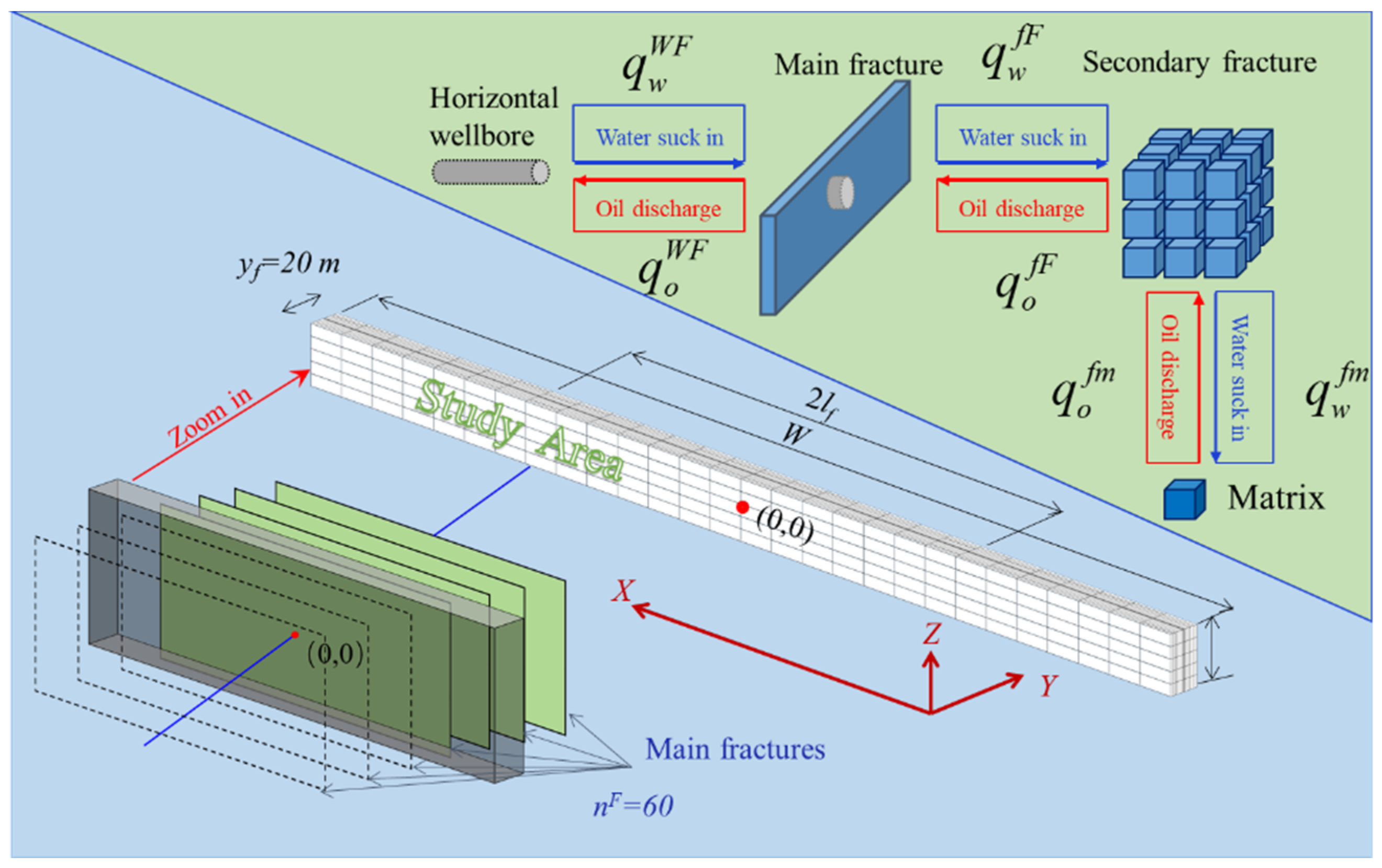
2.1. Assumptions and Physical Model

Assumptions: ① Fractured shale reservoir is composed of the wellbore (W), main fracture (F), secondary fracture (f) and shale substrate (m). The wellbore is the source and sink, and the reservoir exchanges fluid with the outside world through the wellbore; ② considering oil-water two-phase flow. Fluid is slightly compressible; ③ considering the compressibility of fracture and reservoir substrate; ④ considering capillary imbibition; ⑤ the main fractures are discrete vertical fractures with the same height as the reservoir thickness, and the two wings of the main fracture are symmetrically distributed on both sides of the horizontal wellbore; ⑥ the fluid flow is isothermal seepage. A constant fluid temperature has been assumed throughout the flow area.

Based on the above assumptions, the horizontal well model of multi-stage fracturing tight oil can be simplified as a combination of a horizontal wellbore, hydraulic fracture network and substrate system, which are continuously coupled by flow and pressure at the contact surface. Taking a single fracturing stage as an example, the schematic diagram of wellbore, fracture and substrate division is shown in the lower left corner of Figure 1. X, Y and Z are used to represent the three directions of the model grid division. The main fractures are symmetrically distributed vertical fractures, characterized by dense grids with high conductivity, and their sizes are defined by the length, width and height of the fractures. Secondary fractures are vertical fractures orthogonal to the main fractures, which are characterized by fracture density proposed by Yan et al. [19]. The horizontal wellbore is connected with the hydraulic main fracture, and the main fracture, secondary fracture and shale substrate are connected with each other in pairs. After the pump is stopped during the fracturing operation, the oil-water replacement between media is shown in the upper right corner of Figure 1.

2.2. Mathematical Model

The conservation equation of water phase matter is:

$$\begin{array}{l}\frac{\mathsf{\partial }({\rho }_{\mathrm{w}}{\varphi }^{\mathrm{F}}{S}_{\mathrm{w}}^{\mathrm{F}})}{\mathsf{\partial }t}+\frac{\mathsf{\partial }({\rho }_{\mathrm{w}}{\varphi }^{\mathrm{f}}{S}_{\mathrm{w}}^{\mathrm{f}})}{\mathsf{\partial }t}+\frac{\mathsf{\partial }({\rho }_{\mathrm{w}}{\varphi }^{\mathrm{m}}{S}_{\mathrm{w}}^{\mathrm{m}})}{\mathsf{\partial }t}=\nabla \left[\frac{k^{\mathrm{F}}{k}_{\mathrm{rw}}^{\mathrm{F}}{\rho }_{\mathrm{w}}}{{\eta }_w}\nabla \left(p_{\mathrm{w}}^{\mathrm{F}}-{\rho }_{\mathrm{w}}\mathrm{g}D\right)\right]\\ +\nabla \left[\frac{k^{\mathrm{f}}{k}_{\mathrm{rw}}^{\mathrm{f}}{\rho }_{\mathrm{w}}}{{\eta }_{\mathrm{w}}}\nabla \left(p_{\mathrm{w}}^{\mathrm{f}}-{\rho }_{\mathrm{w}}\mathrm{g}D\right)\right]+\nabla \left[\frac{k^{\mathrm{m}}{k}_{\mathrm{rw}}^{\mathrm{m}}{\rho }_{\mathrm{w}}}{{\eta }_{\mathrm{w}}}\nabla \left(p_{\mathrm{w}}^{\mathrm{m}}-{\rho }_{\mathrm{w}}\mathrm{g}D\right)\right]+{\widehat{q}}_{\mathrm{w}}\end{array}$$

(1)

where ${\rho }_{\mathrm{w}}$ is the density of water phase, kg/m³; ${\varphi }^{\mathrm{F}}$, ${\varphi }^{\mathrm{f}}$, ${\varphi }^{\mathrm{m}}$ are the porosity of main fracture, secondary fracture and substrate respectively, dimensionless; $S_{\mathrm{w}}^{\mathrm{F}}$, $S_{\mathrm{w}}^{\mathrm{f}}$, $S_{\mathrm{w}}^{\mathrm{m}}$ are the water saturation of main fracture, secondary fracture and substrate respectively, dimensionless; $k^{\mathrm{F}}$, $k^{\mathrm{f}}$, $k^{\mathrm{m}}$ are the absolute permeability of main fracture, secondary fracture and substrate respectively, m²; $k_{\mathrm{rw}}^{\mathrm{F}}$, $k_{\mathrm{rw}}^{\mathrm{f}}$, $k_{\mathrm{rw}}^{\mathrm{m}}$ are the relative permeability of water phase of main fracture, secondary fracture and substrate respectively, dimensionless; $p_{\mathrm{w}}^{\mathrm{F}}$, $p_{\mathrm{w}}^{\mathrm{f}}$, $p_{\mathrm{w}}^{\mathrm{m}}$ are the water phase pressure of main fracture, secondary fracture and substrate respectively, pa; ${\eta }_{\mathrm{w}}$ is the viscosity of water phase, Pa·s; $\mathrm{g}$ is the acceleration of gravity, g/m²; $D$ is the longitudinal migration distance of fluid, m; ${\widehat{q}}_{\mathrm{w}}$ is the injection flow rate of the water phase, kg/(m³·s).

The conservation equation of oil phase matter is:

$$\begin{array}{l}\frac{\mathsf{\partial }({\rho }_{\mathrm{o}}{\varphi }^{\mathrm{F}}{S}_{\mathrm{o}}^{\mathrm{F}})}{\mathsf{\partial }t}+\frac{\mathsf{\partial }({\rho }_{\mathrm{o}}{\varphi }^{\mathrm{f}}{S}_{\mathrm{o}}^{\mathrm{f}})}{\mathsf{\partial }t}+\frac{\mathsf{\partial }({\rho }_{\mathrm{o}}{\varphi }^{\mathrm{m}}{S}_{\mathrm{o}}^{\mathrm{m}})}{\mathsf{\partial }t}=\nabla \left[\frac{k^{\mathrm{F}}{k}_{\mathrm{ro}}^{\mathrm{F}}{\rho }_{\mathrm{o}}}{{\eta }_{\mathrm{o}}}\nabla \left(p_{\mathrm{o}}^{\mathrm{F}}-{\rho }_{\mathrm{o}}\mathrm{g}D\right)\right]\\ +\nabla \left[\frac{k^{\mathrm{f}}{k}_{\mathrm{ro}}^{\mathrm{f}}{\rho }_{\mathrm{o}}}{{\eta }_{\mathrm{o}}}\nabla \left(p_{\mathrm{o}}^{\mathrm{f}}-{\rho }_{\mathrm{o}}\mathrm{g}D\right)\right]+\nabla \left[\frac{k^{\mathrm{m}}{k}_{\mathrm{ro}}^{\mathrm{m}}{\rho }_{\mathrm{o}}}{{\eta }_{\mathrm{o}}}\nabla \left(p_{\mathrm{o}}^{\mathrm{m}}-{\rho }_{\mathrm{o}}\mathrm{g}D\right)\right]-{\widehat{q}}_{\mathrm{o}}\end{array}$$

(2)

where ${\rho }_{\mathrm{o}}$ is the density of oil phase, kg/m³; $S_{\mathrm{o}}^{\mathrm{F}}$, $S_{\mathrm{o}}^{\mathrm{f}}$, $S_{\mathrm{o}}^{\mathrm{m}}$ are the oil saturation of main fracture, secondary fracture and substrate respectively, dimensionless; $k_{\mathrm{ro}}^{\mathrm{F}}$, $k_{\mathrm{ro}}^{\mathrm{f}}$, $k_{\mathrm{ro}}^{\mathrm{m}}$ are the relative permeability of oil phase of main fracture, secondary fracture and substrate respectively, dimensionless; $p_{\mathrm{o}}^{\mathrm{F}}$, $p_{\mathrm{o}}^{\mathrm{f}}$, $p_{\mathrm{o}}^{\mathrm{m}}$ are the oil phase pressure of main fracture, secondary fracture and substrate respectively, pa; ${\eta }_{\mathrm{o}}$ is the viscosity of oil phase, Pa·s; ${\widehat{q}}_{\mathrm{o}}$ is the flow rate of oil phase between wellbore and main fracture, kg/(m³·s).

The inflow and outflow of fluids exist between two adjacent media, but they cancel each other out in the above conservation equation. The amount of water phase channeling between media can be expressed as follows:

$$q_{\mathrm{w}}^{\mathrm{WF}}=\frac{{\alpha }_1{\rho }_{\mathrm{w}}{k}^{\mathrm{F}}{k}_{\mathrm{rw}}^{\mathrm{F}}(p_{\mathrm{wf}}-p_{\mathrm{w}}^{\mathrm{F}})}{{\eta }_{\mathrm{w}}}$$

(3)

$$q_w^{\mathrm{Ff}}=\frac{{\alpha }_2{\rho }_{\mathrm{w}}{k}^{\mathrm{f}}{k}_{\mathrm{rw}}^{\mathrm{f}}(p_{\mathrm{w}}^{\mathrm{F}}-p_{\mathrm{w}}^{\mathrm{f}})}{{\eta }_{\mathrm{w}}}$$

(4)

$$q_w^{\mathrm{fm}}=\frac{{\alpha }_3{\rho }_{\mathrm{w}}{k}^{\mathrm{m}}{k}_{\mathrm{rw}}^{\mathrm{m}}(p_{\mathrm{w}}^{\mathrm{f}}-p_{\mathrm{w}}^{\mathrm{m}})}{{\eta }_{\mathrm{w}}}$$

(5)

where, $q_{\mathrm{w}}^{\mathrm{WF}}$ is the water phase channeling flow between wellbore and main fracture, kg/(m³·s); ${\alpha }_1$, ${\alpha }_3$, ${\alpha }_3$ are the shape factors between wellbore and main fracture, main fracture and secondary fracture, and secondary fracture and substrate respectively, m⁻²; $p_{\mathrm{wf}}$ is bottom-hole flowing pressure, pa; $q_{\mathrm{w}}^{\mathrm{Ff}}$ is the water phase channeling between the main fracture and the secondary fracture, kg/(m³·s); $q_{\mathrm{w}}^{\mathrm{fm}}$ is the water phase channeling between the secondary fracture and the substrate, kg/(m³·s).

In this paper, Yan et al. [19] combined the discrete fracture network with the dual medium model and established the relationship between the number of fractures per unit area, and the shape factor between the secondary fractures and the substrate to characterize the secondary fracture density formed by tight oil reservoir fracturing.

Considering the compressibility of fractures and substrate pores, it is necessary to supplement the stress sensitivity equations of porosity and permeability:

$${\varphi }^{\mathrm{F}/\mathrm{f}/\mathrm{m}}={\varphi }_0^{\mathrm{F}/\mathrm{f}/\mathrm{m}}{\mathrm{e}}^{C_{\varphi }^{\mathrm{F}/\mathrm{f}/\mathrm{m}}(p_{\mathrm{o}}^{\mathrm{F}/\mathrm{f}/\mathrm{m}}-p_0)}$$

(6)

$$k^{\mathrm{F}/\mathrm{f}/\mathrm{m}}=k_0^{\mathrm{F}/\mathrm{f}/\mathrm{m}}{\mathrm{e}}^{d^{\mathrm{F}/\mathrm{f}/\mathrm{m}}(p_{\mathrm{o}}^{\mathrm{F}/\mathrm{f}/\mathrm{m}}-p_0)}$$

(7)

where ${\varphi }^{\mathrm{F}/\mathrm{f}/\mathrm{m}}$ is the porosity of main fracture/secondary fracture/substrate, dimensionless; ${\varphi }_0^{\mathrm{F}/\mathrm{f}/\mathrm{m}}$ is the initial porosity of main fracture/secondary fracture/substrate, dimensionless; $C_{\varphi }^{\mathrm{F}/\mathrm{f}/\mathrm{m}}$ is porosity compression coefficient of main fracture/secondary fracture/substrate, pa⁻¹; $p_{\mathrm{o}}^{\mathrm{F}/\mathrm{f}/\mathrm{m}}$ is the oil phase pressure of main fracture/secondary fracture/substrate, pa; $p_0$ is the original formation pressure, pa; $k^{\mathrm{F}/\mathrm{f}/\mathrm{m}}$ is the absolute permeability of main fracture/secondary fracture/substrate, m²; $k_0^{\mathrm{F}/\mathrm{f}/\mathrm{m}}$ is the initial permeability of main fracture/secondary fracture/substrate, m²; $d^{\mathrm{F}/\mathrm{f}/\mathrm{m}}$ is the stress sensitivity coefficient of main-fracture/secondary-fracture/substrate determined by experiments [20], pa⁻¹. Due to the relationship between porosity and permeability of fractured reservoir given by Raghavan and Chin [21], the parameter value of $d^{f/m}/C_{\varphi }^{f/m}$ investigated range from 3.0 to 10.0 [22].

For main hydraulic fractures, the relationship between porosity and permeability of main fractures is given by Wang [23]

$$k^F=k_0^F{\left({\varphi }^F/{\varphi }_0^F\right)}^3$$

(8)

Based on the dilation-compaction rule of hydraulic fractures [24], the variation of main-fracture width during the pump-stopping pressure drop can be expressed as follows:

$$w^F=\sqrt[3]{12\tau \frac{k^F}{h^F{n}^F}}$$

(9)

where, w^F and h^F are the width and height of the main fracture respectively, m; τ is the main fracture tortuosity, dimensionless; n^F is the number of fracture clusters.

Considering the oil-water two-phase seepage in fracture and substrate, it is necessary to supplement the constraint equation of water saturation:

$$S_{\mathrm{w}}^{\mathrm{F}/\mathrm{f}/\mathrm{m}}+S_{\mathrm{o}}^{\mathrm{F}/\mathrm{f}/\mathrm{m}}=1$$

(10)

where, $S_{\mathrm{w}}^{\mathrm{F}/\mathrm{f}/\mathrm{m}}$ is the water saturation of main fracture/secondary fracture/substrate, dimensionless; $S_{\mathrm{o}}^{\mathrm{F}/\mathrm{f}/\mathrm{m}}$ is the oil saturation of main fracture/secondary fracture/substrate, dimensionless.

In addition, because the permeability of the main fracture is relatively large, its capillary force is approximately zero, and the substrate has capillary force, which is expressed as:

$$p_{\mathrm{o}}^{\mathrm{F}/\mathrm{f}}=p_{\mathrm{w}}^{\mathrm{F}/\mathrm{f}}$$

(11)

$$p_{\mathrm{o}}^{\mathrm{m}}-p_{\mathrm{w}}^{\mathrm{m}}=p_{\mathrm{c}}^{\mathrm{m}}$$

(12)

where, $p_{\mathrm{o}}^{\mathrm{F}/\mathrm{f}}$ is the oil phase pressure of main fracture/secondary fracture, pa; $p_{\mathrm{w}}^{\mathrm{F}/\mathrm{f}}$ is the water phase pressure of main fracture/secondary fracture, pa; $p_{\mathrm{c}}^{\mathrm{m}}$ is capillary force of substrate, Pa.

2.3. The Initial and Boundary Conditions

It is assumed that the initial pressure and initial water saturation of substrate and fracture are the same, which are undeveloped original reservoir conditions.

The inner boundary shows the fluid exchange volume between the bottom hole and the main fracture. In the fracturing pumping stage of this model, constant pressure injection is simulated, and the pumping volume of the fracturing fluid is calculated according to the following formula:

$${\widehat{q}}_{\mathrm{w}}=\frac{2\mathsf{\pi }{K}^{\mathrm{F}}{K}_{\mathrm{rw}}^{\mathrm{F}}{\rho }_{\mathrm{w}}}{{\eta }_{\mathrm{w}}^{}{B}_{\mathrm{w}}\ln \left(\frac{r_{\mathrm{e}}}{r_{\mathrm{w}}}+S\right)\Delta x\Delta z}\left(p_{\mathrm{wf}}-p_{\mathrm{w}}^{\mathrm{F}}\right)$$

(13)

where, $B_w$ is the volume coefficient of the water phase, m³/m³; $r_e$ is the radius of the supply edge, m; $r_w$ is the radius of the well, m; $S$ is skin factor; $\Delta x$, $\Delta z$, which are the grid sizes of the numerical model in the x direction and z direction, respectively, m.

The selected calculation unit satisfies the closed outer boundary condition:

$$\frac{\mathsf{\partial }p}{\mathsf{\partial }\mathrm{n}}\left|\mathrm{\Gamma }\right.=0$$

(14)

where, $\mathrm{\Gamma }$ is the outer boundary of the shale reservoir; n is the normal direction of the outer boundary.

2.4. Solving Method

The mathematical model is discretized by the finite difference method. The difference format of time and space is processed by pre-difference and central difference, respectively. The implicit method is used to characterize unknown quantities; the semi-implicit method is used to deal with nonlinear coefficient terms and linearize them. Based on the upstream weight method, the conductivity is selected. After substituting the initial and boundary conditions, extract the coefficient substrate. Based on the Gauss–Seidel iterative solution, the unknown values of this time step can be obtained. Repeat the steps to obtain the value of the next step until the set calculation time is reached.

3. Numerical Simulation of Pump-Stopping Pressure Drop

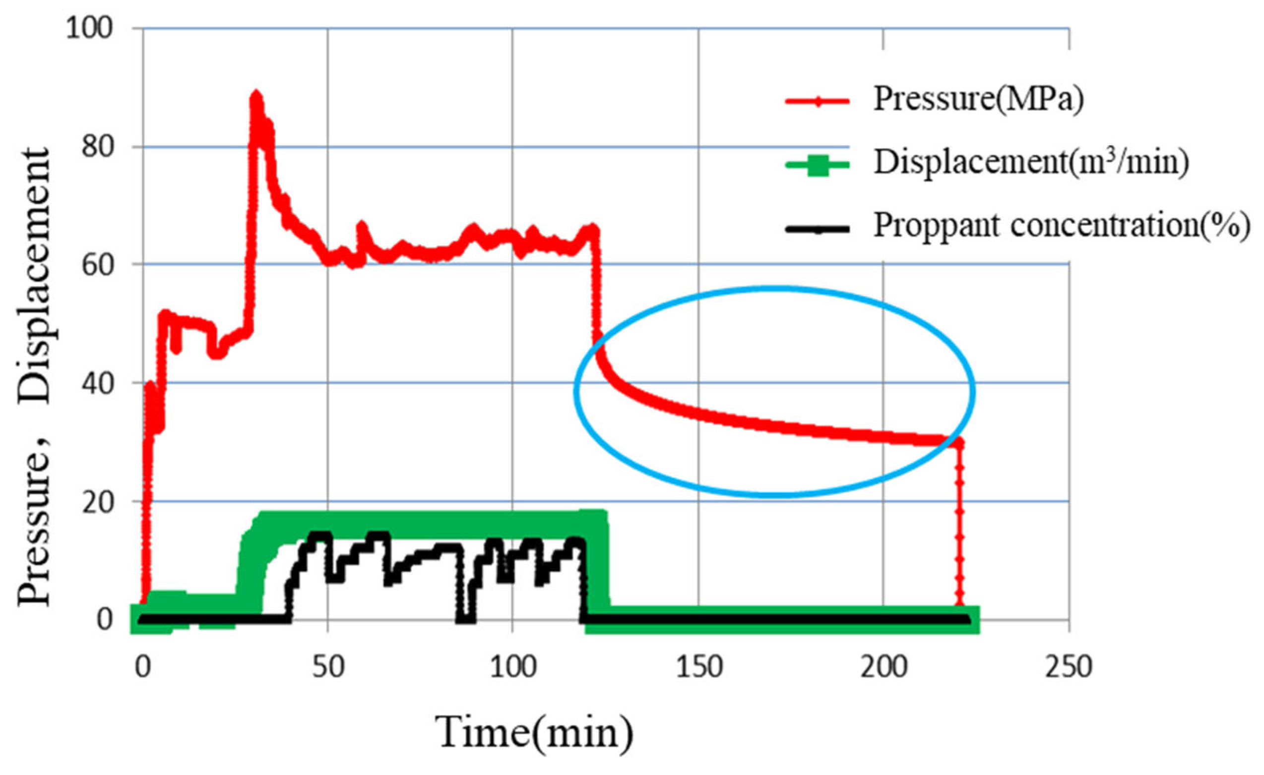
3.1. The Description of Simulated Fracturing Stage

The simulated fracturing stage is established according to the geological and operation parameters of a fracturing stage of a typical tight oil fracturing horizontal well in Junggar Basin, China. The fractured reservoir thickness is 42 m, the well spacing is 500 m, the original pressure is 38 MPa, the substrate initial porosity is 0.086, the substrate initial permeability is 0.007 mD, and the substrate stress sensitivity coefficient is 0.189 MPa⁻¹. The interval between fracturing stages is 40 m, with 3 clusters in each stage. The half-length of the main fracture is 140 m, the flow conductivity of the fracture is 5 D·cm and the stress sensitivity coefficient of the main fracture is 0.12 mpa⁻¹. Secondary fracture initial permeability is 0.1 mD, secondary fracture initial porosity is 0.15, secondary fracture stress sensitivity coefficient is 0.06 MPa⁻¹ and secondary fracture density is 1.1/m². All the reservoir and fracture parameters are determined by lab experiments from the field.

In this model, the oil-water relative permeability and capillary pressure of shale substrate are obtained by core experiment. The fracturing pump injection is simulated as a water injection process, with an injection time of 2 h and an injection volume of 1450 m³. By adjusting the stress sensitivity coefficient of fracture porosity and permeability, the injection rate and injection volume of fracturing fluid are consistent with the actual situation. After pumping, the pressure and water saturation obtained at the end time are taken as initial values to simulate the pressure drop for one day.

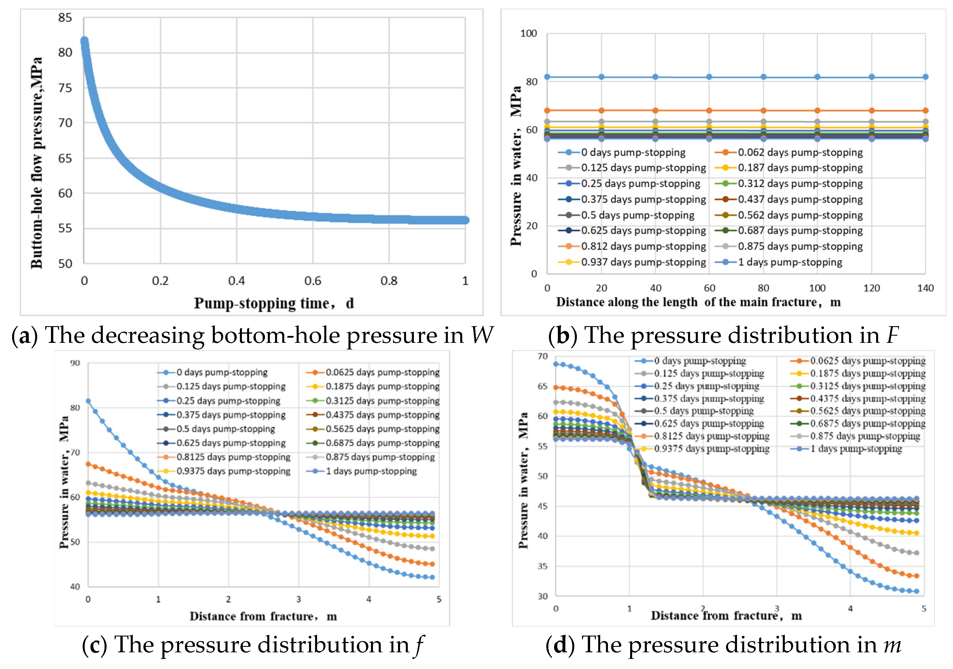
3.2. Simulated Pressure Dynamics

Figure 2 shows the simulated pressure distribution in the quadruple media of bottom-hole-main fracture-secondary fracture-substrate as a function of pump stop time. Figure 2a shows that the bottom hole pressure decreases from 82 MPa at the initial time of termination of pumping to 56 MPa one day after termination of pumping, showing the characteristics of rapid decline at the initial stage and slow decline at the later stage. Figure 2b shows the pressure field distribution in the main fracture along the fracture length direction at different times when the pump is stopped. It can be seen that due to the high conductivity of the main fracture, there is no obvious pressure difference in the main fracture along the fracture length direction, and it shows a pressure-decreasing law consistent with the flowing pressure at the bottom hole. Figure 2c shows the distribution of the pressure field secondary fractures, it can be seen that the pressure of secondary fractures near the main fracture end rises to 81.5 MPa at the initial time of pump stop, but the pressure at the far end only rises to 42 MPa. With the extension of pump stop time, the pressure distribution in secondary fractures shows a changing trend of decreasing near the main fracture end and rising far from the main fracture end, and the internal pressure of secondary fractures tends to be in a balanced state one day after pump stop. Figure 2d shows the distribution of the pressure field in the substrate at different times when the pump is stopped. The substrate pressure near the end of the main fracture rises to 69 MPa at the initial time when the pump is stopped. With the increase in the distance along the wall surface of the main fracture, the pressure gradually drops until it tends to be flat, which shows that the pressure is constantly spreading to the far end to increase the energy of the formation. On the first day after termination of pumping, the pressure inside the stroma did not reach the equilibrium state, but the distal stroma pressure increased from 31 MPa at the initial time of termination of pumping to 46 MPa.

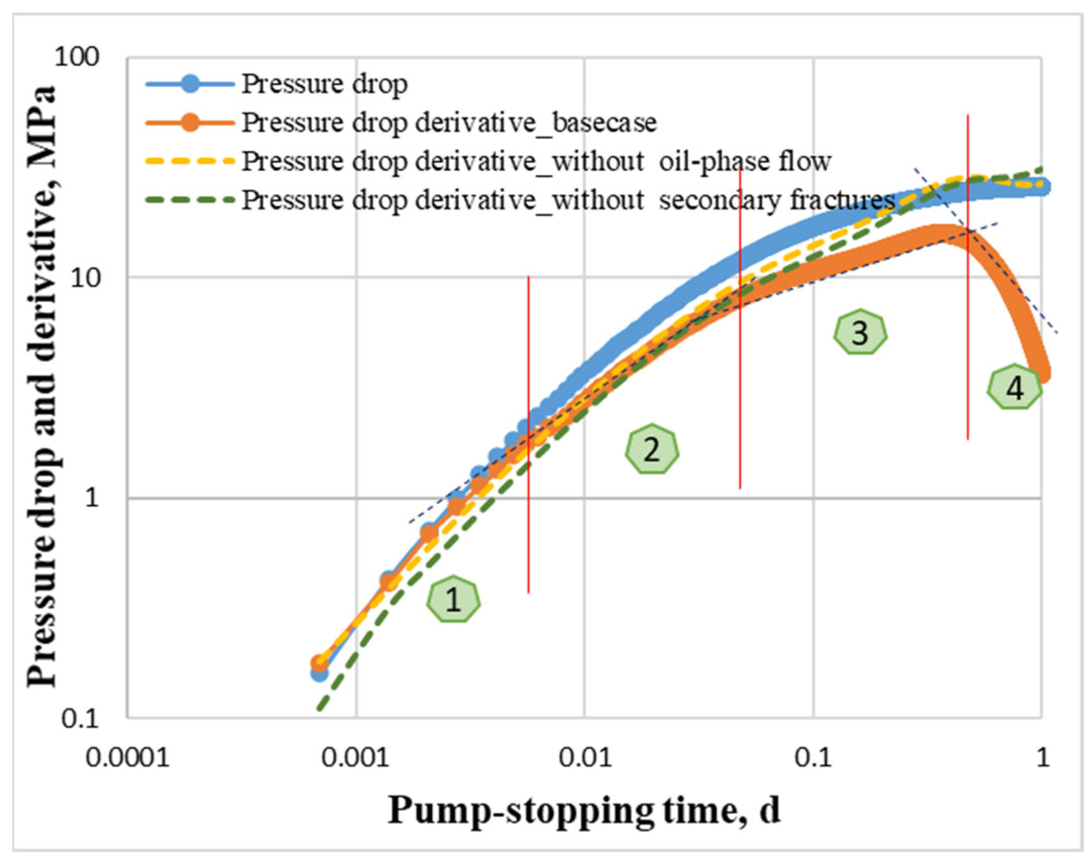
3.3. Simulated Bottom-Hole Pressure Drop

Figure 3 shows the simulated follow-up rate of fracturing fluid in the wellbore to the main fracture, the crossflow rate inside the fracture network system, the leak-off rate of fracturing fluid in the fracture network to the substrate and the oil exchange rate of the substrate to the fracture during the pressure drop from the end of pumping to one day after termination of pumping. The simulation results show that at the initial time when the pump is stopped, the phenomenon of shaft follow-up flow is obvious, and then the flow speed drops rapidly to a very low value. The fracturing fluid in the main fracture will further cross-flow to the secondary fracture and filter to the substrate during the pump stop. With the extension of pump stop time, the crossflow rate in the fracture decreases continuously, until it is surpassed by the leak-off rate in the later stage. Crude oil in the substrate is displaced into the fracture from the initial moment when the pump is stopped, and the speed is very low, but it keeps a steady downward trend all the time. From about 0.53 days when the pump was stopped, the rate of substrate sucking fracturing fluid (leak-off rate) and the rate of crude oil replacing showed a synchronous downward trend.

Figure 4 is a log-log plot of pressure drop and its natural logarithmic derivative drawn by the bottom-hole flowing pressure data simulated in Figure 2a. By associating the simulated bottom-hole pressure drop characteristics with the flow rate between media, the pressure drop during termination of pumping in fracturing operation can be divided into four main control flow stages, which are as follows according to the sequence of termination of pumping time:

• Main fracture reservoir control stage: the fracturing fluid in the wellbore enters the main fracture after termination of pumping, showing that the pressure drop and derivative curves coincide and the slope is 1;
• Inter-fracture crossflow control stage: the fracturing fluid in the fracture system is crossflow between the main fracture and the secondary fracture, the crossflow speed exceeds the bottom hole after flow speed, and the main fracture begins to close, showing that the slope of the pressure drop derivative curve is 1/2;
• The leak-off control stage of the seam net: the rate of the bottom hole after flow and crossflow between the seams decreased rapidly, and the leak-off rate of the seam net to the substrate began to exceed the bottom hole after flow, showing that the slope of the pressure drop derivative curve was 1/4;
• Substrate imbibition and displacement control stage: the leak-off rate of the slot network begins to exceed the crossflow rate between slots, the secondary fractures begin to close, and the substrate oil change rate and the leak-off rate of slot network begin to show a synchronous downward trend, showing that the slope of pressure drop derivative curve is −1. The closing pressure can be calculated from the pressure drop corresponding to the start time of this stage.

Figure 4. The simulated bottom-hole pressure drop and derivative on log-log plot. 1 is Main fracture reservoir control stage; 2 is Inter-fracture crossflow control stage; 3 is The leak-off control stage of the seam net; 4 is Substrate imbibition and displacement control stage.

Figure 4. The simulated bottom-hole pressure drop and derivative on log-log plot. 1 is Main fracture reservoir control stage; 2 is Inter-fracture crossflow control stage; 3 is The leak-off control stage of the seam net; 4 is Substrate imbibition and displacement control stage.

To investigate the impact of secondary fractures and two-phase flow on the pressure drop, we first set the porosity and permeability of secondary fractures in the base case model to be consistent with the matrix pores, in order to simulate the situation without secondary fractures. Again, we set the initial oil saturation in the oil reservoir being zero in the base case model to simulate the situation without oil-phase flow. The two sets of pressure drop derivative curves (green for without secondary fractures and yellow for without oil-phase flow) are simulated using the same pumping schedule with the base case model mentioned above, as shown in Figure 4. The two sets of pressure drop derivative curves no longer exhibit “1-1/2-1/4-negative 1” four-slope-shaped characteristics.

They both present a single slope with just a slight difference in the early stages.

4. Field Applications

The model is applied to the fracturing operation of the 28th stage of X1, a tight oil horizontal well in the Junggar basin. As shown in Figure 5, the half-length of the main fracture is 92 m, the diversion capacity of the main fracture is 8.8 D·cm, the secondary fracture density is 1.05/m², the substrate permeability is 0.001 mD, and the closing pressure is 69.8 MPa the fitting effect is shown in Figure 6.

In order to verify the rationality of the interpretation results of the model in this paper, the pressure drop analysis of fracturing operation data of the 28th stage of Well X1 was completed by using the classic commercial software Saphir–Minifrac, version number is V.5.20.03.08, as shown in Figure 7. The Minifrac pressure drop model does not consider secondary fractures and migration of oil and water. The half-length of fractures and substrate permeability explained by the mini frac model is 144.10 m and 0.0241 mD, far exceeding the interpretation results of the model in this paper, and the interpretation results of permeability exceed the average permeability values of cores measured on site. Comparing the interpretation results of the two groups, it shows that the interpretation results of the pressure drop model with secondary fractures and oil-water displacement are more realistic.

On this basis, this model is applied to the pressure drop data of the other 15 fracturing stages of Well X1. The operation pressure of each fracturing stage of Well X1 is shown in Figure 8. The pressure drop data of each stage are fitted by stage, and the parameters such as half-length of main fracture, conductivity, secondary fracture density, closure pressure and substrate permeability are obtained by inversion. The fitting interpretation results of each fracturing stage are counted as shown in Figure 9. Inversion shows that the half-length of main fractures in each fracturing stage is 83.88–95.79 m, the conductivity of main fractures is 7.24–9.78 D·cm, the density of secondary fractures is 0.96–1.18 /m², the closing pressure is 68.26–82.77 MPa, and the substrate permeability is 0.001–0.002 mD. The fracture parameters and reservoir parameters of each fracturing stage explained by pressure drop fitting reflect the non-uniform transformation effect of tight oil horizontal well X1 after large-scale hydraulic fracturing, which provides a basis for accurately establishing a non-uniform fracture productivity model for productivity prediction and system optimization.

For validating the model, fracture parameters obtained by pressure drop fitting are compared with the results of micro-seismic monitoring, shown in Figure 10, Figure 11 and Figure 12. Due to the differences in parameter interpretation accuracy and principles [25], the main-fracture half-length and secondary-fracture density from our model are different from the values from micro-seismic monitoring. However, the variation trend of these two parameters in each fracturing stage is consistent with the results from micro-seismic monitoring, which demonstrates the effectiveness of our model.

5. Conclusions

In this paper, a pumping-stop pressure drop model is presented considering the hydraulic fracture network and water-oil flow during the pump shutdown. Numerical simulation and field case application for a hydraulically fractured tight oil well are also conducted using the proposed model. Our main conclusions are as follows:

(1)

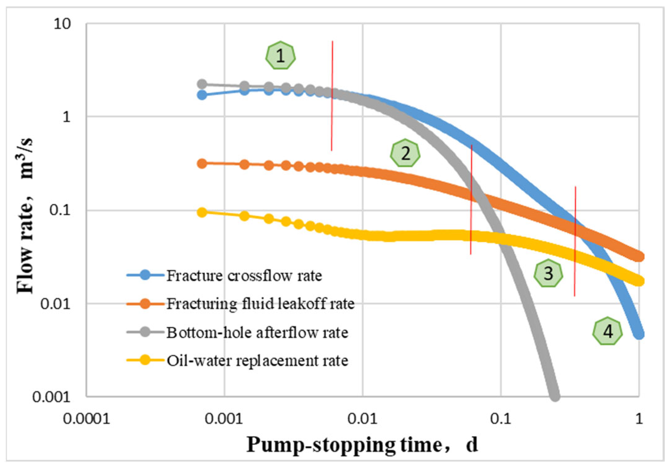
It is found by numerical simulation that the rate of wellbore afterflow is the largest at the initial time of pump stop, which is dominant in all flows, and then drops rapidly to a very low value. The fracturing fluid in the main fracture will further cross-flow to the secondary fracture and filter to the substrate during the pump stops. With the extension of pump stop time, the leak-off rate of fracturing fluid in the later stage will surpass other flow rates and become the dominant factor. Crude oil in the substrate will be displaced into the fracture from the initial moment when the pump is stopped, and the oil replacement rate is very low but steadily declining, and will be synchronized with the leak-off rate in the later stage.

(2)

According to the correlation with the flow rate among media during the pump shutdown, the pressure drop during the pump shutdown in fracturing operation is divided into four main control flow stages, which are: main fracture reservoir control stage, inter-fracture crossflow control stage, fracture net leak-off control stage and substrate imbibition and replacement control stage according to the sequence of pump stop time.

(3)

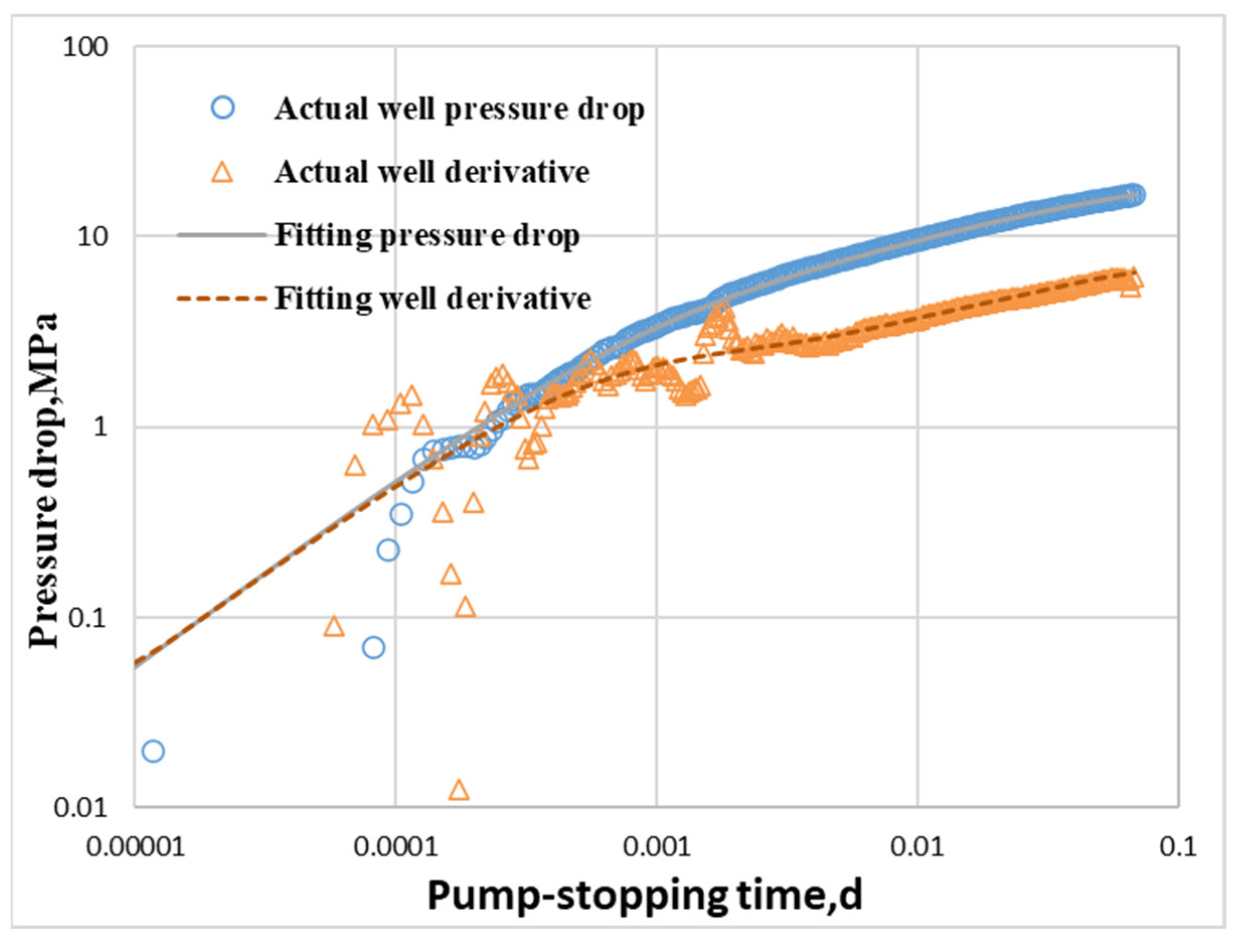
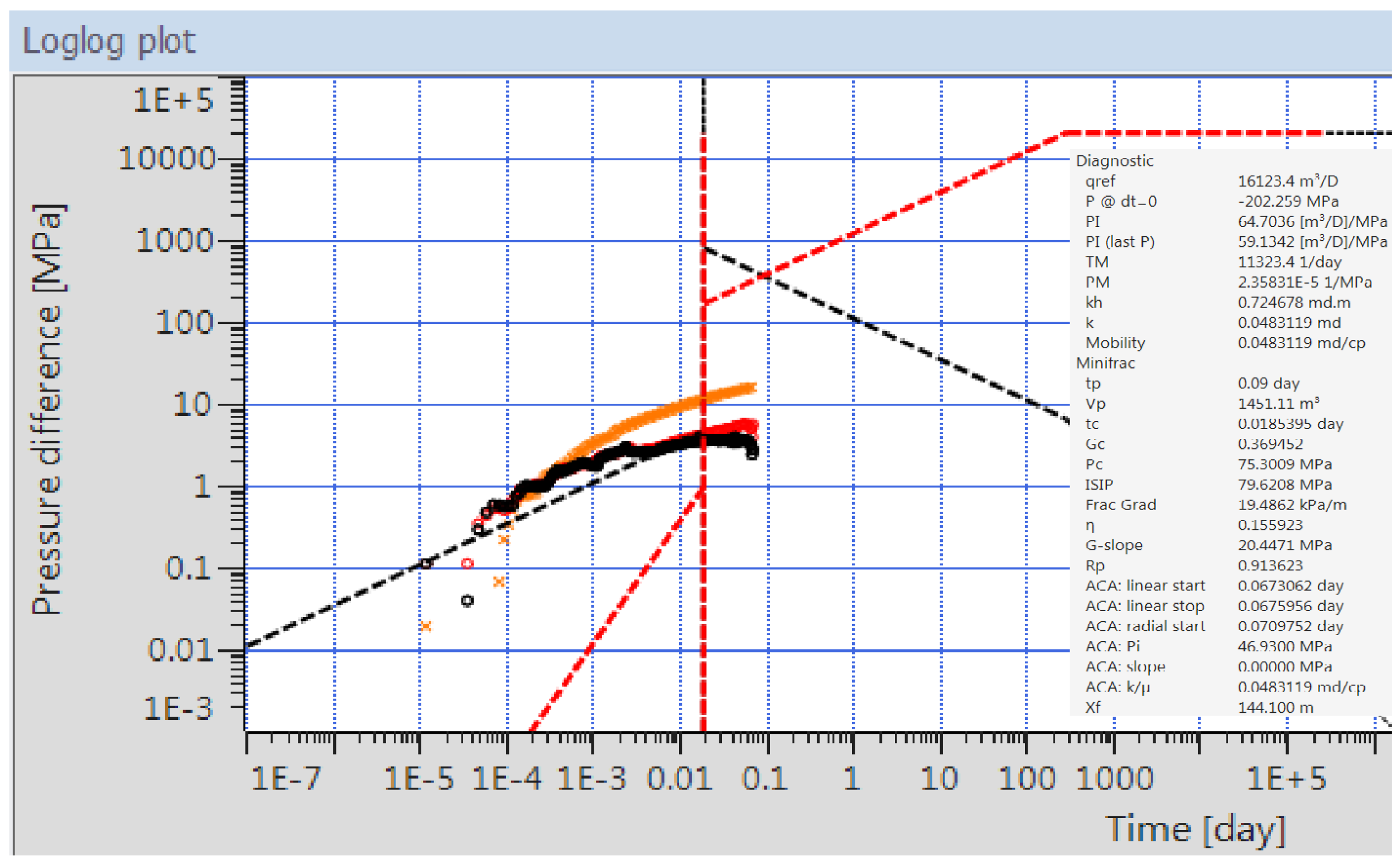
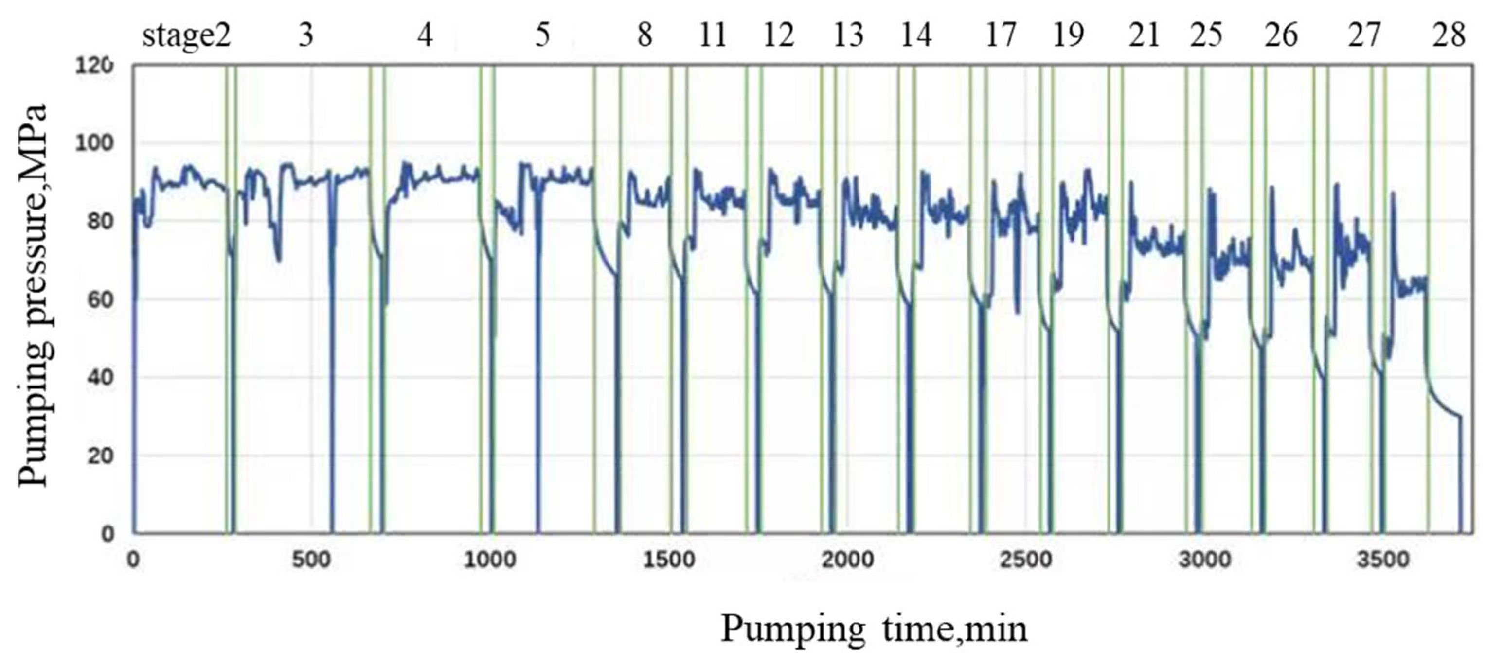
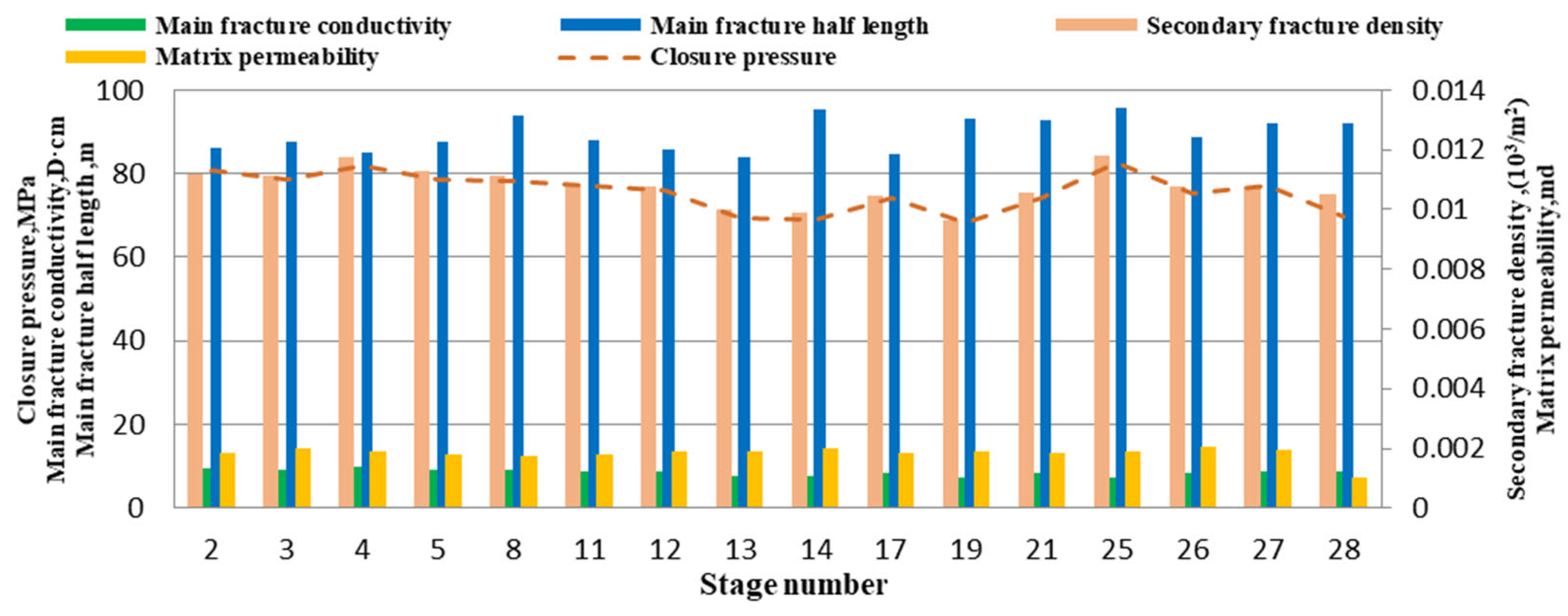
By fitting the actual fracturing data with the proposed pressure drop model, the key parameters such as fracture network parameters (including half-length of main fracture, conductivity and density of secondary fracture), and closure pressure of each fracturing stage can be obtained by inversion. Compared with the commercial software Saphir–Minifrac model which does not consider the secondary fracture and oil exchange effect, the interpretation results of the proposed model are more accurate and reasonable. In addition, the practical application of well X1 shows that the pressure drop model proposed in this paper can be used to finely evaluate the effect of heterogeneous reoperation in each fracturing stage of horizontal wells.

References

1. Nolte, K.G. Determination of proppant and fluid schedules from fracturing-pressure decline. SPE Prod. Eng. 1986, 1, 255–265. [Google Scholar] [CrossRef]
2. Valko′, P.P.; Economides, M.J. Fluid-leakoff delineation in high-permeability fracturing. SPE Prod. Facil. 1999, 14, 110–116. [Google Scholar] [CrossRef]
3. Talley, G.R.; Swindell, T.M.; Waters, G.A.; Nolte, K.G. Field application of after-closure analysis of fracture calibration tests. In Proceedings of the SPE Mid-Continent Operations Symposium, Oklahoma City, OK, USA, 28–31 March 1999. [Google Scholar]
4. Denney, D. Estimating pore pressure and permeability in massively stacked lenticular reservoirs. J. Pet. Technol. 1999, 51, 52–53. [Google Scholar] [CrossRef]
5. Mohamed, I.M.; Azmy, R.M.; Sayed, M.; Marongiu-Porcu, M.; Ehlig-Economides, C.A. Evaluation of after-closure analysis techniques for tight and shale gas formations. In Proceedings of the SPE Hydraulic Fracturing Technology Conference, The Woodlands, TX, USA, 24–26 January 2011. [Google Scholar]
6. Marongiu-Porcu, M.; Ehlig-Economides, C.A.; Economides, M.J. Global model for fracture falloff analysis. In Proceedings of the SPE North American Unconventional Gas Conference and Exhibition, The Woodlands, TX, USA, 24–26 January 2011. [Google Scholar]
7. Ma, J.; Zhao, J.; Lin, Y.; Liang, J.; Chen, J.; Chen, W.; Huang, L. Study on Tamped Spherical Detonation-Induced Dynamic Responses of Rock and PMMA Through Mini-chemical Explosion Tests and a Four-Dimensional Lattice Spring Model. Rock Mech. Rock Eng. 2023, 10, 7357–7375. [Google Scholar] [CrossRef]
8. Ma, J.; Chen, J.; Chen, W.; Huang, L. A coupled thermal-elastic-plastic-damage model for concrete subjected to dynamic loading. Int. J. Plast. 2022, 153, 103279. [Google Scholar] [CrossRef]
9. Ma, J.; Chen, J.; Guan, J.; Lin, Y.; Chen, W.; Huang, L. Implementation of Johnson-Holmquist-Beissel model in four-dimensional lattice spring model and its application in projectile penetration. Int. J. Impact Eng. 2022, 170, 104340. [Google Scholar] [CrossRef]
10. Soliman, M.Y. Technique for considering fluid compressibility and temperature changes in mini-frac analysis. In Proceedings of the SPE Annual Technical Conference and Exhibition, New Orleans, LA, USA, 5–8 October 1986. [Google Scholar]
11. Soliman, M.Y.; Miranda, C.; Wang, H.M. Application of after-closure analysis to a dual-porosity formation, to CBM, and to a fractured horizontal well. SPE Prod. Oper. 2010, 25, 472–483. [Google Scholar] [CrossRef]
12. Urbanowicz, K.; Bergant, A.; Kodura, A.; Kubrak, M.; Malesińska, A.; Bury, P.; Stosiak, M. Modeling Transient Pipe Flow in Plastic Pipes with Modified Discrete Bubble Cavitation Model. Energies 2021, 14, 6756. [Google Scholar] [CrossRef]
13. Wang, Y.P.; Sun, L.; Zhang, S.C.; Chen, L.; Liu, P.; Chen, Z. Pressure-decline curve analysis method and its application in fracture reservoir. J. China Univ. Pet. 2004, 28, 55–57. [Google Scholar]
14. Mao, G.Y.; Yang, H.C.; Zhang, W.Z. Pressure drowdown analysis method and its application in fractured reservoir. J. Oil Gas Technol. 2011, 33, 116–118+122. [Google Scholar]
15. Liu, S.J.; Cai, J.J.; Wang, F.; Lv, X.R.; Wang, W. Application of improved pressure decline analysis for fracturing in offshore low permeability gas field. Fault-Block Oil Gas Field 2015, 22, 369–373. [Google Scholar]
16. Liu, G.; Ehlig-Economides, C. Interpretation methodology for fracture calibration test before-closure analysis of normal and abnormal leakoff mechanisms. In Proceedings of the SPE Hydraulic Fracturing Technology Conference, The Woodlands, TX, USA, 9–11 February 2016. [Google Scholar]
17. Liu, G.; Ehlig-Economides, C. Practical considerations for diagnostic fracture injection test (DFIT) analysis—ScienceDirect. J. Pet. Sci. Eng. 2018, 171, 1133–1140. [Google Scholar] [CrossRef]
18. Karpenko, M.; Stosiak, M.; Šukevičius, Š.; Skačkauskas, P.; Urbanowicz, K.; Deptuła, A. Hydrodynamic Processes in Angular Fitting Connections of a Transport Machine’s Hydraulic Drive. Machines 2023, 11, 355. [Google Scholar] [CrossRef]
19. Yan, B.; Mi, L.; Wang, Y.; Tang, H.; An, C.; Killough, J.E. Mechanistic simulation workflow in shale gas reservoirs. In Proceedings of the SPE Reservoir Simulation Conference, Montgomery, TX, USA, 20–22 February 2017. [Google Scholar]
20. Eshkalak, M.O.; Aybar, U.; Sepehrnoori, K. An integrated reservoir model for unconventional resources, coupling pressure dependent phenomena, SPE-171008-MS. In Proceedings of the SPE Eastern Regional Meeting, Charleston, WV, USA, 21–23 October 2014. [Google Scholar] [CrossRef]
21. Raghavan, R.; Chin, L.Y. Productivity changes in reservoirs with stress-dependent permeability, SPE-77535-MS. In Proceedings of the SPE Annual Technical Conference and Exhibition, San Antonio, TX, USA, 29 September–2 October 2002. [Google Scholar] [CrossRef]
22. Petro, D.R.; Chu, W.; Burk, M.K.; Rogers, B.A. Benefits of pressure transient testing in evaluating compaction effects: Gulf of Mexico deepwater turbidite sands, SPE-38938-MS. In Proceedings of the SPE Annual Technical Conference and Exhibition, San Antonio, TX, USA, 5–8 October 1997. [Google Scholar] [CrossRef]
23. Wang, F.; Pan, Z.; Zhang, Y.; Zhang, S. Simulation of coupled hydro-mechanical-chemical phenomena in hydraulically fractured gas shale during fracturing-fluid flowback. J. Pet. Sci. Eng. 2018, 163, 16–26. [Google Scholar] [CrossRef]
24. Huang, X.; Wang, J.; Chen, S.N.; Gates, I.D. A simple dilation-recompaction model for hydraulic fracturing. J. Unconv. Oil Gas Resour. 2016, 16, 62–75. [Google Scholar] [CrossRef]
25. Maxwell, S.; Deere, J. An introduction to this special section: Microseismic. Lead. Edge 2010, 29, 277. [Google Scholar] [CrossRef]
Figure 1. Schematic diagram of wellbore-fracture network-reservoir oil-water two-phase flow coupling model.
Processes 11 03145 g001
Figure 2. Pressure distribution dynamics in W-F-f-m mediums during the pump-stopping process.
Processes 11 03145 g002
Figure 3. The simulated bottom-hole afterflow rate, fracture crossflow rate, fracturing fluid leakoff rate and oil-water replacement rate. 1 is Main fracture reservoir control stage; 2 is Inter-fracture crossflow control stage; 3 is The leak-off control stage of the seam net; 4 is Substrate imbibition and displacement control stage.
Processes 11 03145 g003
Figure 5. Fracturing operation pressure curve of tight oil well X1 28th stage. The blue line highlights the pressure drop after pump shutdown.
Processes 11 03145 g005
Figure 6. The pressure drop curve is fitted by the model established in this paper.
Processes 11 03145 g006
Figure 7. Results of pressure drop analysis with Saphir–Minifrac software. The red circle is actual well pressure drop, the black circle is actual well derivative, the orange ‘x’ is fitting well derivative.
Processes 11 03145 g007
Figure 8. The fracturing operation pressure of each fracturing stage of tight oil well X1.
Processes 11 03145 g008
Figure 9. Pressure drop fitting results of each fracturing stage of tight oil well X1.
Processes 11 03145 g009
Figure 10. Micro-seismic monitoring results of hydraulically fractured tight oil well X1. The circle symbol stand for the Micro-seismic monitoring results. Different color stand for the different stage.
Processes 11 03145 g010
Figure 11. Comparison of main-fracture half-lengths between micro-seismic monitoring and pressure drop fitting.
Processes 11 03145 g011
Figure 12. Comparison of secondary-fracture density and micro-seismic events.
Processes 11 03145 g012
Disclaimer/Publisher’s Note: The statements, opinions and data contained in all publications are solely those of the individual author(s) and contributor(s) and not of MDPI and/or the editor(s). MDPI and/or the editor(s) disclaim responsibility for any injury to people or property resulting from any ideas, methods, instructions or products referred to in the content.