A Robust Control for a Controllable Suspension System with an Input Time Delay

Abstract

In this study, a state feedback robust control strategy with time delay dependence for the uncertainty, fault, and input time delay of a vehicle’s controllable suspension system is designed. Firstly, based on the working principle of the adjustable damping suspension system, the total damping force of the suspension is divided into “foundation damping force” and “controllable damping force”, taking the adjustable damping interval as the constraint boundary, which varies with the actuating velocity. Furthermore, based on the sensitivity analysis of the input time delay’s relationship with damping force disturbance, it exerts influence on the controllable damping force part. The associated uncertainty and fault are defined through linear fraction transformation and proportional gain, respectively, and the two are decoupled from the control mechanism. Then, based on the Lyapunov stability theory, a robust control law for the time-delay-dependent H∞ state feedback is designed and transformed into a linear matrix inequality convex optimization problem to solve. Finally, the feasibility and effectiveness of the proposed method are verified by designing different combinations of uncertainty and fault tests and by comparing and analyzing these with the time-delay-independent H2/H∞ robust control strategy under random and pulse road excitation.

1. Introduction

The vehicle suspension system plays an essential role in vehicle dynamics, improving ride comfort and road holding [1]. Apart from carrying the vehicle body, it can also adequately guarantee stability and provide passengers with as much comfort as possible, isolating road vibration and shock. Based on whether it can be controlled externally, it can be classified as a passive vehicle suspension system (V-PSS) [2] or a controllable vehicle suspension system (V-CSS) [3,4]. V-PSSs are challenging in terms of balancing ride comfort and handling stability since these performance requirements are always in conflict; but, V-CSSs, which use different controls, are a compelling technical scheme [5]. However, in addition to performance optimization control, any V-CSS will inevitably have unexpected perturbation uncertainties and faults in the service process, affecting the system’s dynamic performance quality and stability. In order to make the system insensitive to such perturbation uncertainties and faults, a robust fault-tolerant control is needed. Considering this, extensive research has been carried out on topics such as state feedback passive robust fault-tolerant control [6,7], adaptive robust fault-tolerant control [8], sky-hook fault-tolerant control [9], linear variable parameter control (LPV) [10,11], linear variable parameter model predictive control (LPV-MPC) [12], adaptive fault-tolerant control via the T-S fuzzy method [13], H2/H∞ passive robust fault-tolerant control [14], hybrid control of state feedback compensation and nominal state feedback [15], constrained adaptive backstep tracking controllers [16], H∞ passive robust fault-tolerant control based on output feedback [17], adaptive state feedback robust fault-tolerant control [18], and fault-tolerant prescribed performance control [19]. The above-mentioned research has achieved excellent results. Nevertheless, these studies mainly focused on parametric perturbed uncertainties and actuator faults, ignoring the time delay that objectively exists in any controllable system. In fact, the time delay introduced by a control system also affects the dynamic performance and stability of the system. It reflects the fact that the sensor signal transmission, control calculation, and actuator response require a certain amount of time to occur, inevitably leading to an unavoidable time delay. The dominant delay is the time interval between the actuator receiving the control command and the expected output damping force [20], which is also the input time delay of the system control force (referred to as the “input time delay” in this paper). When the actuator receives the control instruction, it does not immediately output the control force required by the system but generates it after some time has passed. A time delay can cause the actuator output control force to be out of sync with the control force required by the system, possibly resulting in system instability or performance deterioration [21]. However, the above studies on robust fault-tolerant control of suspension systems do not consider the influence of input time delay [6,7,8,9,10,11,12,13,14,15,16,17,18,19]. Moreover, there is a wealth of existing research on the time delay control of suspension systems, including adaptive backward-step time delay control [21], H∞ state feedback time delay control [22,23], H∞ output feedback time delay control [24], and fuzzy static output feedback (SOF) time delay control based on parallel distributed compensation (PDC) [25]. However, these do not introduce faults. Furthermore, related control studies in the control field purpose methods such as a delay-kernel-dependent approach for handling the nonlinear saturation function and sufficient LMI conditions to solve the saturated controller problem [26]. An auxiliary system with free singularity was designed to overcome input saturation and the saturation compensation control law was proposed to ameliorate the negative effects of input saturation [27,28]. These studies provide some inspiration for research on the control approach. However, further consideration is needed based on the dynamic characteristics of V-CSSs.

In summary, the industry has conducted in-depth studies on fault-tolerant control in V-CSSs [6,7,8,9,10,11,12,13,14,15,16,17,18,19] considering system faults. Time delay control [21,22,23,24,25] explores the effect of a system time delay. However, in any V-CSS, a time delay can objectively be said to exist when a fault occurs. The input time delay is inherent in systems with controllability and the fault occurs due to the accumulation of the service time of the system. The combined effect of the delay and the fault will further worsen the problem. Furthermore, according to whether the actuator can actively generate force, V-CSSs can be classified as having semi-active suspension or active suspension. Semi-active suspension is more widely used due to its cost and energy consumption advantages. Suspension systems with adjustable damping are based on the real-time control of the damping force of the adjustable shock absorber to match different dynamic performance requirements. The actuating velocity and the controllable damping coefficient determine the damping force. Both are time-dependent and jointly determine the output force. Compared with active suspension, the damping force and suspension controllable force are coupled in semi-active suspension. It is necessary to simultaneously consider the impact of the time delay and faults in semi-active suspension systems. The existing literature on this subject mainly focuses on active suspension [29,30,31,32] but the methods for active suspension are only partially suitable for semi-active suspension.

In addition, among the above studies on fault-tolerant control, both passive fault-tolerant control [6,7,14,17], following the idea of “responding to all changes with no changes” and active fault-tolerant control [8,13,16,18], based on the principle of “changing to change”, are included, both of which have their advantages and disadvantages. Although the design of passive fault-tolerant control is conservative, when the delay factor is introduced into fault-tolerant control, the improvement it brings to the system’s overall dynamic performance and stability can compensate for the performance loss caused by conservatism. For example, the control architecture can prevent the time delay caused by fault diagnosis and control law reorganization in the active fault-tolerant control method [27]. Taking an adjustable damping suspension system as the research object, the passive fault-tolerant control method is adopted in this study to design a control system based on robust control, so it is appropriate to define it as robust control here. The strategy considering the input time delay is studied to ensure the dynamic performance and stability of the system. The major contributions of this study are as follows:

(1) Based on the working principle of an adjustable damping suspension system, the total damping force of the suspension is divided into two parts, “foundation damping force” and “controllable damping force”, and the adjustable damping interval, which varies with actuating speed, is taken as the constraint boundary of the total damping force. Unlike in previous works [9,11,12], based on an analysis of the sensitivity of the input time delay to damping force disturbance, it is confirmed that its influence is concentrated on the controllable damping force and the associated uncertainty and faults are defined by linear fraction transformation and proportional gain, respectively, to realize their decoupling from the control mechanism.

(2) Unlike previous studies on control methods for V-CSSs with partial consideration of the uncertainty, faults, and input time delay [6,7,8,9,10,11,12,13,14,15,16,17,18,19,20,21,22,23,24,25], this study deals with all of the above essential factors, focusing mostly on an adjustable damping suspension system. By introducing the idea of robust control, a time-delay-dependent H∞ state feedback robust control law based on Lyapunov stability theory is designed and transformed into a convex optimization problem of linear matrix inequalities. Constructing the Lyapunov–Krasovskii function proves its stability under the delay type uncertainty, perturbation type uncertainty, and fault. Moreover, utilizing this mechanism, fault diagnosis and control law reorganization in the active fault-tolerant control method are removed such that the complex design procedure and expensive computing pressure are effectively avoided.

(3) In contrast to the existing methods for controlling suspension without considering input time delay [6,7,14,17], we build a time-delay-independent (TDI) control based on ${H_2/H}_{\infty }$ as a comparative method. Based on the two-degrees-of-freedom vehicle suspension model, with input time delay and fault gain as test factors, test combinations with different factor levels are designed and the proposed delay-dependent (TDD) robust control method is compared with the TDI control method and analyzed to verify the feasibility and effectiveness of the proposed method.

The remainder of this paper is organized as follows: in Section 2, we analyze the influence of input delay on the system uncertainty and faults of the V-CSS; in Section 3, we design a time-delay-dependent robust control strategy; in Section 4, we construct and verify the effectiveness of the proposed control strategy; and Section 5 summarizes the research content.

2. Influence of Input Time Delay on Uncertainty and Fault of a V-CSS

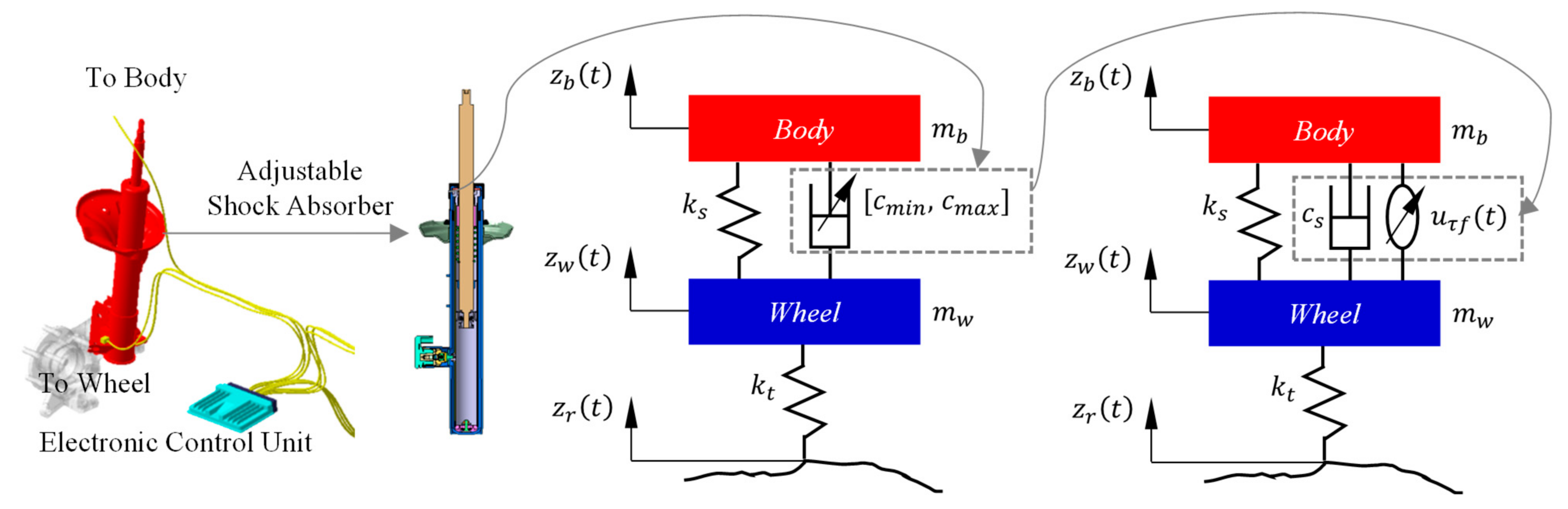
This paper takes an adjustable damping suspension system as the research object, in which the adjustable shock absorber acts as the control actuator and provides the variable damping force required by the system. The variable damping force is determined by the actuating velocity and the controllable damping coefficient (related to the driving current, defined as cur). It is further divided into the recovery damping force and the compression damping force according to the positive and negative values of the actuating velocity. The input time delay is conferred by the controllable system, which refers explicitly to the interval between the adjustable shock absorber receiving the control command and generating the desired control force, leading to a delay in generating the control input force required by the system. The uncertainty and fault refer to the perturbation of the damping force value and the damping force attenuation of the adjustable shock absorber, which occurs with the accumulation of system service time. Regarding variable damping force, relevant studies have shown that it can be divided into foundation damping force and controllable damping force [9,11,12]. Perturbation uncertainty and fault result from parametric perturbation of the suspension system (including the control system), whose influence on foundation damping force cannot be ignored. In practice, more emphasis is placed on the time delay caused by the suspension control system for the uncertainty and fault in the controllable damping force category.

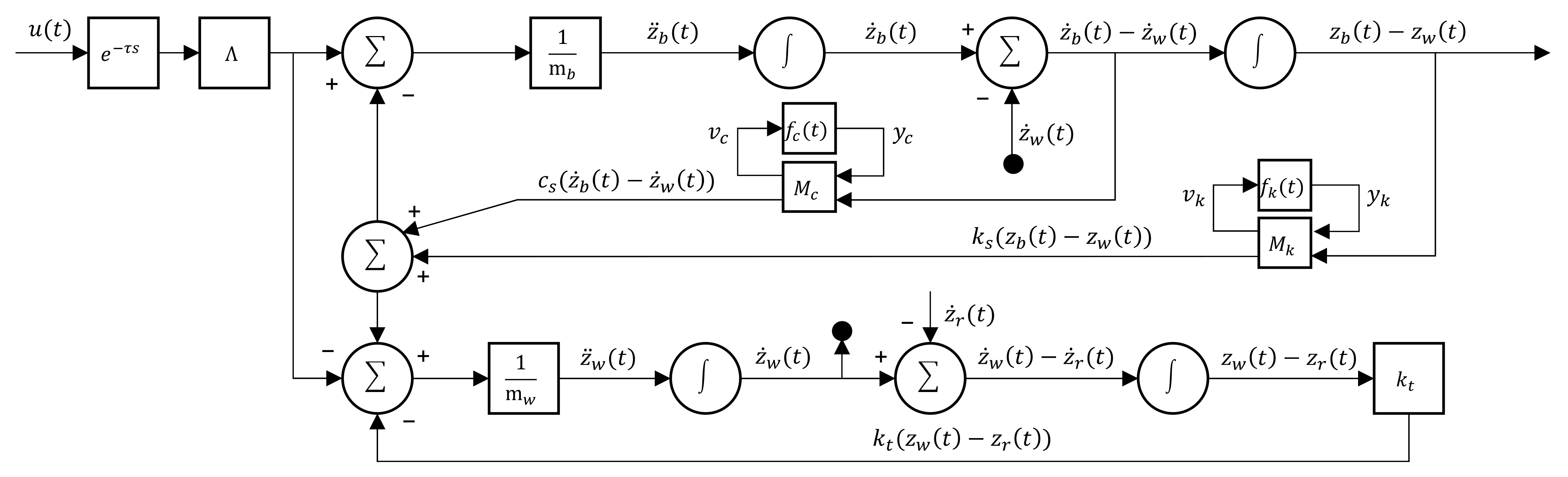
Given this combined with the focus on control strategy here and the aim to simplify the complexity of suspension system dynamics analysis and controller design, a two-degrees-of-freedom vehicle controllable suspension dynamics model, as shown in Figure 1, is constructed and the variable damping effect is divided into two parts.

The differential equation of vehicle controllable suspension motion with two degrees of freedom is shown in Formula (1) [6,9].

$$\left\{\begin{array}{c}{m}_b{\ddot{z}}_b\left(t\right)=-k_s\left(z_b\left(t\right)-z_w\left(t\right)\right)-c_s\left({\dot{z}}_b\left(t\right)-{\dot{z}}_w\left(t\right)\right)+u_{\tau f}\left(t\right)\\ m_w{\ddot{z}}_w\left(t\right)=k_s\left(z_b\left(t\right)-z_w\left(t\right)\right)+c_s\left({\dot{z}}_b\left(t\right)-{\dot{z}}_w\left(t\right)\right)-k_t\left(z_w\left(t\right)-z_r\left(t\right)\right)-u_{\tau f}\left(t\right)\end{array}\right.$$

(1)

where $m_b$ is body mass (the sprung mass) and the unit is kg. ${\ddot{z}}_b$ is the body vertical acceleration and the unit is m/s².$m_w$ is the unsprung mass and the unit is kg. ${\ddot{z}}_w$ is the wheel vertical acceleration and the unit is m/s². $k_t$ is the tire stiffness and the unit is N/m. $z_w$ is the wheel vertical displacement and the unit is m. $z_r$ is the road vertical displacement and the unit is m. $k_s$ is the suspension stiffness and the unit is N/m. $z_b$ is the body vertical displacement and the unit is m. $c_s$ is the foundation damping and the unit is N·s/m.${\dot{z}}_b$ is the body vertical velocity and the unit is m/s. ${\dot{z}}_w$ is the wheel vertical velocity and the unit is m/s. $u_{\tau f}$ is the controllable damping force and the unit is N.

As shown in Figure 1, the damping force of the adjustable shock absorber is divided into $c_s\left({\dot{z}}_b\left(t\right)-{\dot{z}}_w\left(t\right)\right)$ and $u_{\tau f}$ and the relationship between them is shown in Formula (2).

$$c_{min}\left({\dot{z}}_b\left(t\right)-{\dot{z}}_w\left(t\right)\right)\le c_s\left({\dot{z}}_b\left(t\right)-{\dot{z}}_w\left(t\right)\right)+u_{\tau f}\le c_{max}\left({\dot{z}}_b\left(t\right)-{\dot{z}}_w\left(t\right)\right)$$

(2)

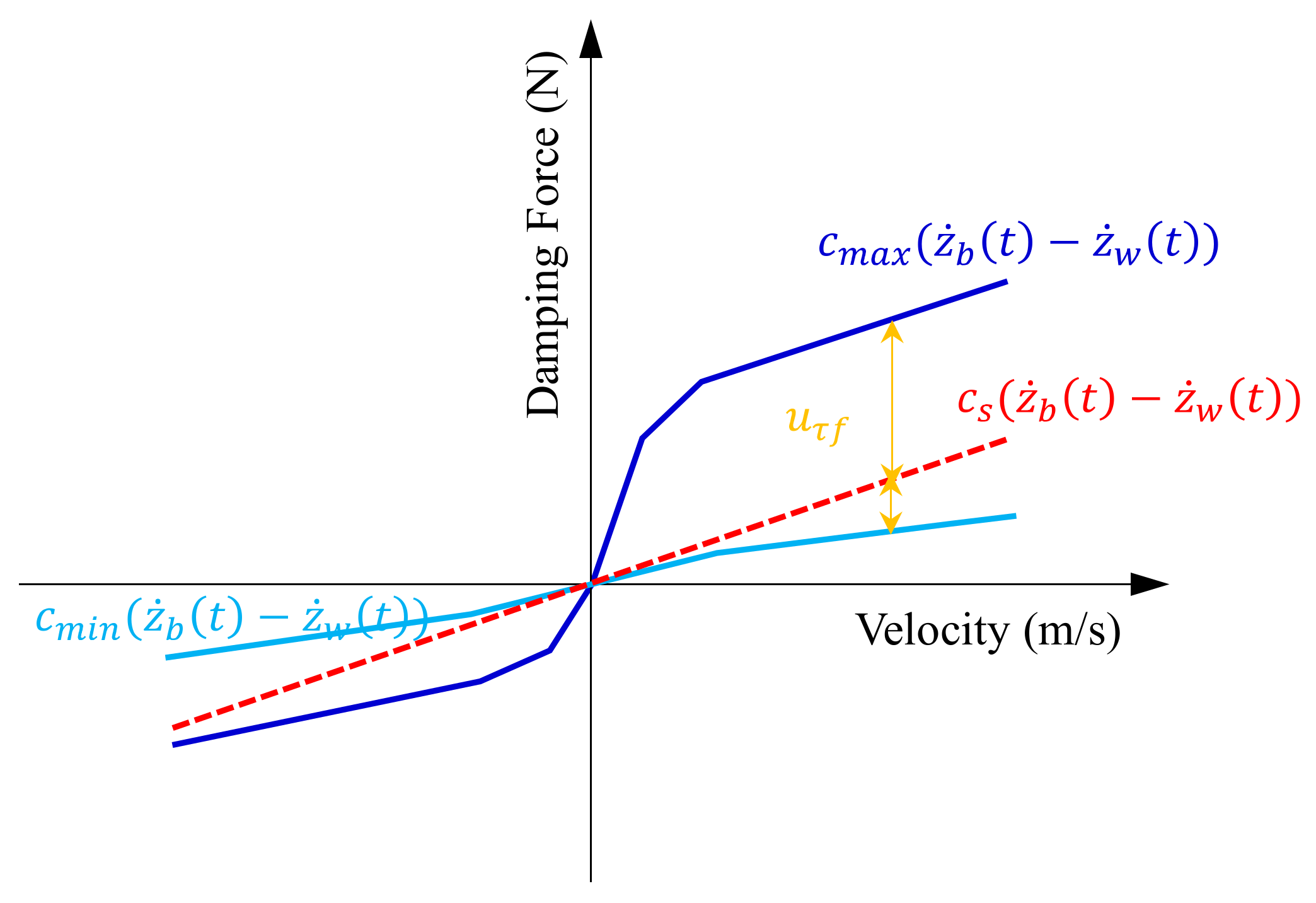
where $c_s$ is defined as a linear value, which is convenient for the control law design. $c_{min}$ and $c_{max}$ are the lower limit and upper limit of the damping coefficient of the adjustable shock absorber, respectively. They are nonlinear values, using the unit N·s/m, and are the value constraints of $u_{\tau f}$, as shown in Figure 2.

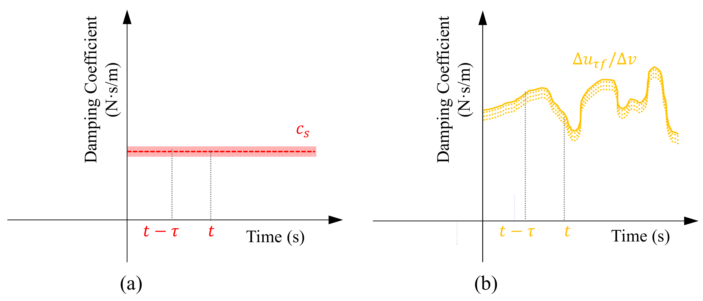
Furthermore, after dividing the variable damping force into two parts, the foundation damping force and the controllable damping force, the correlation between these two parts and the input time delay is analyzed (Figure 3): $c_s\left({\dot{z}}_b\left(t\right)-{\dot{z}}_w\left(t\right)\right)$ is the foundation damping force of the adjustable shock absorber, where the actuating velocity ${\dot{z}}_b\left(t\right)-{\dot{z}}_w\left(t\right)$ is time-varying, but the foundation damping $c_s$ is linear and has a weak correlation with the input time delay, which is mainly affected by the parameter perturbation of the suspension system (including the control system). The controllable damping is strongly related to the input time delay and $u_{\tau f}$ is time-varying and nonlinear. Once the input time delay exists, it will cause the expected damping force and the actual damping force to be out of sync and the final system control force will also be superimposed with the damping force attenuation of the shock absorber. Therefore, the perturbation uncertainty of the variable damping force is associated with the foundation damping force and the input delay and fault are mainly associated with the controllable damping force.

(1) Perturbation uncertainty in foundation damping

Based on the above analysis of the foundation damping force’s characteristics, the foundation damping’s perturbation uncertainty is defined, as shown in Formula (3).

$$c_s={\overline{c}}_s(1+d_c{f}_c(t\left)\right)$$

(3)

where ${\overline{c}}_s$ is the nominal value of suspension foundation damping, $d_c$ is the perturbation value of suspension foundation damping, and $f_c\left(t\right)$ is the time-varying perturbation function, $\left|f_c\left(t\right)\right|\le 1$.

Furthermore, based on the linear fraction transformation [33], Formula (3) can be equivalent to Formula (4).

$$c_s=F_u\left(\left[\begin{array}{cc}0& {\overline{c}}_s\\ d_c& {\overline{c}}_s\end{array}\right],f_c(t)\right)=F_u\left(M_c,f_c\left(t\right)\right)$$

(4)

(2) Input time delay and fault in controllable damping force

Based on the above analysis, the system control force of the input time delay and the fault is defined, as shown in Formula (5).

$$u_{\tau f}=\mathsf{\Lambda }u(t-\tau )$$

(5)

where $u\left(t\right)$ is the nominal input control force, $\tau$ is the control input time delay, $0<\tau <\overline{\tau }$, and $\overline{\tau }$ is the critical delay of the controlled system. $\mathsf{\Lambda }$ is the fault factor, which is defined in Formula (6).

$$\left\{\begin{array}{c}\mathsf{\Lambda }={\mathsf{\Lambda }}_0\left(I+V\right)\\ {\mathsf{\Lambda }}_0={\lambda }_0\\ V=(\sigma -{\lambda }_0)/{\lambda }_0\\ \left|V\right|\le S\le I\\ S={{(\lambda }_u-\lambda }_l)/{{(\lambda }_u+\lambda }_l)\end{array}\right.$$

(6)

where $\sigma$ is the fault gain of the adjustable shock absorber, $\sigma \in \left[\mathrm{0,1}\right]$. ${\lambda }_l$ and ${\lambda }_u$ are the fault factor lower limit and upper limit, respectively. Here, ${{0\le \lambda }_l\le \sigma \le \lambda }_u$, ${{{\lambda }_0=(\lambda }_l+\lambda }_u)/2$, ${\mathsf{\Lambda }}_0$, $S$, $V$ is the intermediate variable, and $I$ is the proper dimensional identity matrix.

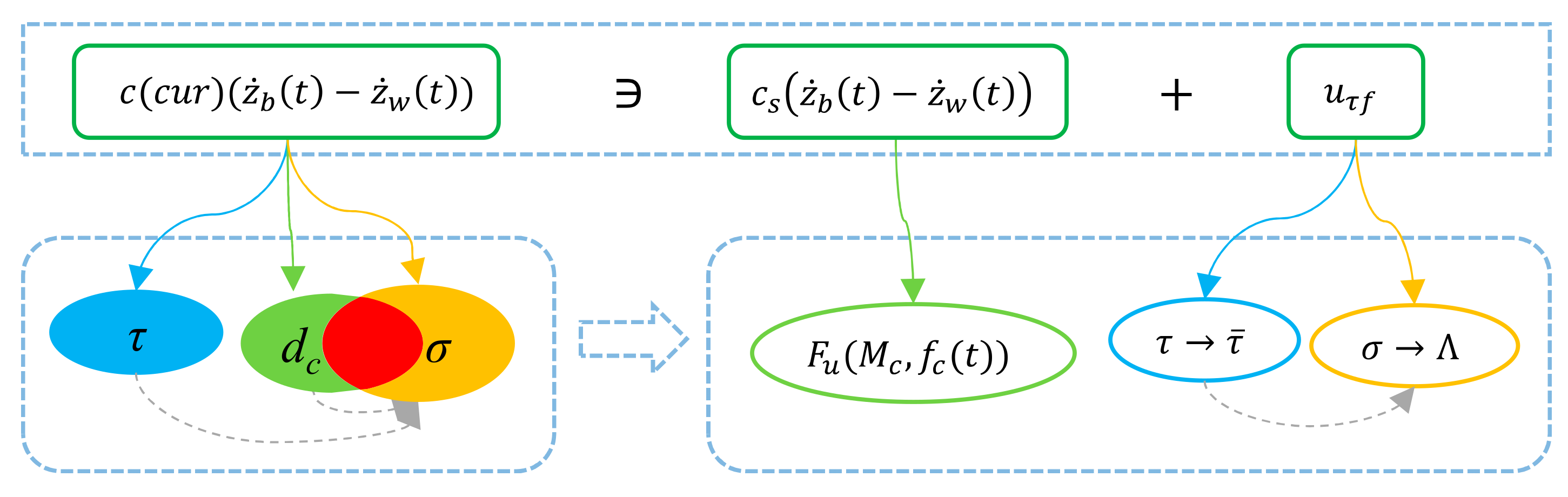
Based on Formula (2), Figure 2, and Formulas (4)–(6) and from the perspective of control method construction, the decoupling between the perturbation uncertainty of the adjustable shock absorber and the fault is realized, as shown in Figure 4. In practice, the parameter perturbation value d_c of the damping force $c\left(cur\right)\left({\dot{z}}_b\left(t\right)-{\dot{z}}_w\left(t\right)\right)$ and the fault gain $\sigma$ overlap. After the conversion of the above definition, the decoupling between the two is realized. However, in the end, their sum is constrained by Formula (2) which is constrained by both time and the actuating velocity of the shock absorber and its constraint relationship is further refined in Formula (7).

In Figure 4, $cur$ is the driving current, the unit is A, $c\left(cur\right)$ represents the adjustable shock absorber damping, where the output is different levels of damping with different driving currents, and $c\left(cur\right)\in [c_{min},c_{max}]$, for which the unit is N·s/m. For Formula (7), set $F_u^{{}^{\prime }}={(c}_{max}-c_s)\left({\dot{z}}_b\left(t\right)-{\dot{z}}_w\left(t\right)\right)$, $F_l^{{}^{\prime }}={(c}_{min}-c_s)\left({\dot{z}}_b\left(t\right)-{\dot{z}}_w\left(t\right)\right)$. $F_u^{{}^{\prime }}$ and $F_l^{{}^{\prime }}$ are the upper and lower limit of controllable damping force, respectively, and the unit is N. $u$ is the input damping force and the unit is N.

$$\left\{\begin{array}{c}{u}_{\tau f}=u when \left({\dot{z}}_b\left(t\right)-{\dot{z}}_w\left(t\right)\right)>0 and F_l^{{}^{\prime }}<u<F_u^{{}^{\prime }}\\ u_{\tau f}=F_l^{{}^{\prime }} when \left({\dot{z}}_b\left(t\right)-{\dot{z}}_w\left(t\right)\right)>0 and F_l^{{}^{\prime }}\ge u\\ u_{\tau f}=F_u^{{}^{\prime }} when \left({\dot{z}}_b\left(t\right)-{\dot{z}}_w\left(t\right)\right)>0 and u\ge F_u^{{}^{\prime }}\\ u_{\tau f}=u when \left({\dot{z}}_b\left(t\right)-{\dot{z}}_w\left(t\right)\right)<0 and F_l^{{}^{\prime }}>u and u>F_u^{{}^{\prime }}\\ u_{\tau f}=F_l^{{}^{\prime }} when \left({\dot{z}}_b\left(t\right)-{\dot{z}}_w\left(t\right)\right)<0 and F_l^{{}^{\prime }}\le u\\ u_{\tau f}=F_u^{{}^{\prime }} when \left({\dot{z}}_b\left(t\right)-{\dot{z}}_w\left(t\right)\right)<0 and u\le F_u^{{}^{\prime }}\end{array}\right.$$

(7)

Similarly, according to Formulas (3) and (4), the suspension stiffness’ perturbation uncertainty is considered, as shown in Formulas (8) and (9).

$$k_s={\overline{k}}_s(1+d_k{f}_k(t\left)\right)$$

(8)

$$k_s=F_u\left(\left[\begin{array}{cc}0& {\overline{k}}_s\\ d_k& {\overline{k}}_s\end{array}\right],f_k(t)\right)=F_u\left(M_k,f_k\left(t\right)\right)$$

(9)

where ${\overline{k}}_s$ is the nominal value of the suspension stiffness, ${\overline{k}}_s$ is the perturbation value of the suspension stiffness, and $f_k\left(t\right)$ is the time-varying perturbation function, $\left|f_k\left(t\right)\right|\le 1$.

Then, based on Formulas (1)–(9), the 2-DOF V-CSS with uncertainty and fault is constructed, as shown in Figure 5.

The state variables $x\left(t\right)$, output variable $z\left(t\right)$, and disturbance input $w\left(t\right)$ are defined in Formula (10).

$$\left\{\begin{array}{c}x(t)={\left[\begin{array}{cccc}{z}_b\left(t\right)-z_w\left(t\right)& {\dot{z}}_b\left(t\right)& z_w\left(t\right)-z_r\left(t\right)& {\dot{z}}_w\left(t\right)\end{array}\right]}^T\\ z\left(t\right)={\mathsf{\omega }}_1\frac{{\ddot{z}}_b\left(t\right)}{{\ddot{z}}_{bmax}}+{\mathsf{\omega }}_2\frac{{\ddot{z}}_w\left(t\right)}{{\ddot{z}}_{wmax}}+{\mathsf{\omega }}_3\frac{z_b\left(t\right)-z_w\left(t\right)}{{{(z}_b-z_w)}_{max}}\\ w\left(t\right)={\dot{z}}_r\left(t\right)\end{array}\right.$$

(10)

where $z\left(t\right)$ is formed by weighting the three key performance objectives of the suspension system (body acceleration, wheel acceleration, and suspension dynamic travel displacement) using the coefficient, where ${\mathsf{\omega }}_1$, ${\mathsf{\omega }}_2$, and ${\mathsf{\omega }}_3$ are the weighting coefficients of each performance indicator. Based on the importance of the three indicators, combined with the order relation method and empirical preference, indicators are ranked as follows: body acceleration > wheel acceleration > suspension dynamic travel displacement. Moreover, r₂ = 1.4 indicates that body acceleration is significantly more critical than wheel acceleration and r₃ = 1.2 indicates that wheel acceleration is slightly more important than suspension dynamic travel displacement. Then, in the substitution into the formula ${\omega }_j={(1+\sum _{k=2}^j\prod _{i=k}^j{r}_i)}^{-1}$, the values are set to 0.4430, 0.3090, and 0.2577, respectively. ${\ddot{z}}_{bmax}$, ${\ddot{z}}_{wmax}$, and ${{(z}_b-z_w)}_{max}$ are the maximum constraints of each performance objective, respectively.

The state space mapping relationship and system state equation are established based on Figure 5.

$$\left[\begin{array}{c}\dot{x}\\ v\\ z\end{array}\right]=\left[\begin{array}{cccc}A& B_y& B_u& B_w\\ C_v& 0& 0& 0\\ C& D_y& D& 0\end{array}\right]\left[\begin{array}{c}x\\ y\\ u\\ w\end{array}\right]$$

(11)

$$\left\{\begin{array}{c}\dot{x}\left(\mathrm{t}\right)=(A+∆A)x\left(t\right)+{(B}_u+∆B_u\left)\mathsf{\Lambda }u\right(t-\tau )+B_{w}w(t)\\ z\left(t\right)=Cx\left(t\right)+D\mathsf{\Lambda }u(t-\tau )\\ x\left(t\right)=\phi \left(t\right), \forall t\in [-\tau ,0]\end{array}\right.$$

(12)

In Formulas (11) and (12), $A$ is a 4 × 4 matrix, $B_y$ is a 4 × 2 matrix, $B_u$ is a 4 × 1 matrix, $B_w$ is a 4 × 1 matrix, $C_v$ is a 2 × 4 matrix, $C$ is a 1 × 4 matrix, $D_y$ is a 1 × 2 matrix, and $D$ is a 1 × 1 matrix. $∆A, ∆B_u$ is an unknown matrix that represents the uncertain parameters of the system and has the following form:

$$\left[\begin{array}{cc}∆A& ∆B_u\end{array}\right]=HF\left(t\right)\left[\begin{array}{cc}{E}_a& E_b\end{array}\right]$$

(13)

In Formula (13), $H$, $E_a$, and $E_b$ are known steady matrices and $H=B_y$, $E_a=C_v$, and $E_b=0$, where $F\left(t\right)$ is the unknown uncertain matrix containing $f_c\left(t\right)$ and $f_k\left(t\right)$; $F\left(t\right)\in L_2[0,+\infty )$, and $F^T\left(t\right)F\left(t\right)\le I$, $I$ form the proper dimensional identity matrix. The matrices are as follows:

$$\begin{gathered} A=\left[\begin{array}{cccc}0& 1& 0& -1\\ \frac{-{\overline{k}}_s}{m_b}& \frac{-{\overline{c}}_s}{m_b}& 0& \frac{{\overline{c}}_s}{m_b}\\ 0& 0& 0& 1\\ \frac{{\overline{k}}_s}{m_w}& \frac{{\overline{c}}_s}{m_w}& \frac{-k_t}{m_w}& \frac{-{\overline{c}}_s}{m_w}\end{array}\right],B_y={\left[\begin{array}{cccc}0& \frac{-d_c}{m_b}& 0& \frac{d_c}{m_w}\\ 0& \frac{-d_k}{m_b}& 0& \frac{d_k}{m_w}\end{array}\right]}^T,B_u={\left[\begin{array}{cccc}0& \frac{1}{m_b}& 0& \frac{-1}{m_w}\end{array}\right]}^T, \\ {B}_w={\left[\begin{array}{cccc}0& 0& -1& 0\end{array}\right]}^T,C_v=\left[\begin{array}{cccc}0& {\overline{c}}_s& 0& {\overline{c}}_s\\ {\overline{k}}_s& 0& 0& 0\end{array}\right],D_y=\left[\begin{array}{cc}\frac{-d_c}{m_b}& \frac{-d_k}{m_b}\end{array}\right],D=\left[\begin{array}{c}\frac{{\mathsf{\omega }}_1}{m_b}-\frac{{\mathsf{\omega }}_2}{m_w,}\end{array}\right] \\ C=\left[\begin{array}{cccc}\frac{-{\mathsf{\omega }}_1{\overline{k}}_s}{m_b}+\frac{{\mathsf{\omega }}_2{\overline{k}}_s}{m_w}+{\mathsf{\omega }}_3& \frac{-{\mathsf{\omega }}_1{\overline{c}}_s}{m_b}+\frac{{\mathsf{\omega }}_2{\overline{c}}_s}{m_w}& \frac{-{\mathsf{\omega }}_2{k}_t}{m_w}& \frac{{\mathsf{\omega }}_1{\overline{c}}_s}{m_b}-\frac{{\mathsf{\omega }}_2{\overline{c}}_s}{m_w}\end{array}\right]. \end{gathered}$$

Furthermore, the state feedback robust control law is defined, as shown in Formula (14).

$$u_{\tau f}=\mathsf{\Lambda }Kx\left(t-\tau \right)$$

(14)

where $K$ is the state feedback gain matrix. Then, Formula (15) is rewritten as

$$\left\{\begin{array}{c}\dot{x}\left(\mathrm{t}\right)=(A+∆A)x\left(t\right)+{(B}_u+∆B_u\left)\mathsf{\Lambda }Kx\right(t-\tau )+B_{w}w(t)\\ z\left(t\right)=Cx\left(t\right)+D\mathsf{\Lambda }Kx(t-\tau )\\ x\left(t\right)=\phi \left(t\right), \forall t\in [-\tau ,0]\end{array}\right.$$

(15)

3. Time-Delay-Dependent Robust Control Law of a V-CSS

Based on the V-CSS with uncertainty and faults established in the previous section and the definition and analysis of its inherent uncertainty and fault characteristics, robust control of the V-CSS is constructed considering the influence of input time delay. Specifically, a passive fault-tolerant control method is adopted. Implementing the idea of “responding to all changes with no changes” at the beginning of the design can prevent the time delay caused by fault diagnosis and control law recombination in the active fault-tolerant control method. Moreover, with the help of a robust control idea, the control system can be made insensitive to the input time delay and fault to ensure the system’s performance and stability.

A state feedback robust control law like Formula (14) is designed for a closed-loop system; see Formula (15). Considering the uncertainty and fault of the suspension system, system Formula (15) satisfies the following conditions under the disturbance input signal $w\left(t\right)\in L_2[0,\infty )$ with limited energy:

(1) The system is asymptotically stable under external input interference;

(2) For a given anti-interference coefficient $\gamma$, in the case of the zero initial value, the closed-loop system shown in Formula (15) should ensure that ${‖z\left(t\right)‖}_2<{\gamma ‖w\left(t\right)‖}_2$.

According to the feedback control law in Formula (14) and the closed-loop system in Formula (15), the necessary conditions (Theorem) for the existence of the time-delay-dependent $H_{\infty }$ robust controller and the related proof process are given.

Theorem 1.

Given anti-interference coefficient$\gamma$, the closed-loop system (15) is asymptotically stable with$\forall \overline{\tau }$satisfying$0<\overline{\tau }<\tau$if there exist positive definite symmetric matrices $L$, $M$, and$N$and proper dimensional matrices $P$, $Q$, $R$, and $\epsilon >0$, $\beta >0$, satisfying matrix inequalities (16) and (17). Moreover, the time-delay-dependent H∞ robust control law is given by$Kx\left(t-\tau \right)=R{L}^{-1}x(t-\tau )$.

$$s.t.\left[\begin{array}{ccccccc}{\mathsf{\Phi }}_{11}& {\mathsf{\Phi }}_{12}& B_w& {\mathsf{\Phi }}_{14}& {\mathsf{\Phi }}_{15}& {\mathsf{\Phi }}_{16}& 0\\ \mathrm{*}& -N& 0& \tau R^T{\mathsf{\Lambda }}_0^T{B}_u^T& R^T{\mathsf{\Lambda }}_0^T{\mathrm{D}}^T& R^T{\mathsf{\Lambda }}_0^T{E}_b^T& R^T{S}^{1/2}\\ \mathrm{*}& \mathrm{*}& -{\gamma }^{2}I& \tau B_w^T& 0& 0& 0\\ \mathrm{*}& \mathrm{*}& \mathrm{*}& {\mathsf{\Phi }}_{44}& {\mathsf{\Phi }}_{45}& {\mathsf{\Phi }}_{46}& 0\\ \mathrm{*}& \mathrm{*}& \mathrm{*}& \mathrm{*}& {\mathsf{\Phi }}_{55}& {\mathsf{\Phi }}_{56}& 0\\ \mathrm{*}& \mathrm{*}& \mathrm{*}& \mathrm{*}& \mathrm{*}& {\mathsf{\Phi }}_{66}& 0\\ \mathrm{*}& \mathrm{*}& \mathrm{*}& \mathrm{*}& \mathrm{*}& \mathrm{*}& -\beta I\end{array}\right]<0$$

(16)

$$s.t.\left[\begin{array}{cc}P& Q\\ Q^T& L{M}^{-1}L\end{array}\right]>0$$

(17)

where ${\mathsf{\Phi }}_{11}=L{A}^T+AL+\tau P+Q+Q^T+N+\epsilon H{H}^T+\beta B_u{\mathsf{\Lambda }}_{0}S{\mathsf{\Lambda }}_0^T{B}_u^T$, ${\mathsf{\Phi }}_{12}=B_u{\mathsf{\Lambda }}_{0}R-Q$, ${\mathsf{\Phi }}_{14}=\tau L{A}^T+\epsilon \tau H{H}^T+\beta B_u{\mathsf{\Lambda }}_{0}S{\mathsf{\Lambda }}_0^T{B}_u^T$, ${\mathsf{\Phi }}_{15}=L{C}^T+\beta B_u{\mathsf{\Lambda }}_{0}S{\mathsf{\Lambda }}_0^T{D}^T$, ${\mathsf{\Phi }}_{16}=L{E}_a^T+\beta B_u{\mathsf{\Lambda }}_{0}S{\mathsf{\Lambda }}_0^T{E}_b^T$, ${\mathsf{\Phi }}_{44}=-\tau M+\epsilon {\tau }^{2}H{H}^T+\beta {\tau }^2{B}_u{\mathsf{\Lambda }}_{0}S{\left(B_u{\mathsf{\Lambda }}_0\right)}^T$, ${\mathsf{\Phi }}_{45}=\beta \tau B_u{\mathsf{\Lambda }}_{0}S{\left(D{\mathsf{\Lambda }}_0\right)}^T$, ${\mathsf{\Phi }}_{46}=\beta \tau B_u{\mathsf{\Lambda }}_{0}S{\left(E_b{\mathsf{\Lambda }}_0\right)}^T$, ${\mathsf{\Phi }}_{55}=-I+\beta D{\mathsf{\Lambda }}_{0}S{\left(D{\mathsf{\Lambda }}_0\right)}^T$, ${\mathsf{\Phi }}_{56}=\beta D{\mathsf{\Lambda }}_{0}S{\left(E_b{\mathsf{\Lambda }}_0\right)}^T$, and ${\mathsf{\Phi }}_{66}=-\epsilon I+{\beta E}_b{\mathsf{\Lambda }}_{0}S{\left(E_b{\mathsf{\Lambda }}_0\right)}^T$.

Lemma 1

[34]. If the vector $a(·)\in R^m$, $b(·)\in R^m$, and $N_1\in R^{m\times n}$ defined within the interval $\Omega$, for $\forall X_1, Y_1, and Z_1\in R^{m\times n}$ the following is satisfied:

$$\mathrm{If} \left[\begin{array}{cc}{X}_1& Y_1\\ Y_1^T& Z_1\end{array}\right]>0, \mathrm{then}-2{\int }_{\mathsf{\Omega }}^{}{a}^T\left(\theta \right)N_{1}b\left(\theta \right)d\theta \le {\int }_{\mathsf{\Omega }}^{}{\left[\begin{array}{c}a\left(\theta \right)\\ b\left(\theta \right)\end{array}\right]}^T\left[\begin{array}{cc}{X}_1& Y_1-N_1\\ Y_1^T-N_1^T& Z_1\end{array}\right]\left[\begin{array}{c}a\left(\theta \right)\\ b\left(\theta \right)\end{array}\right]d\theta$$

(18)

Lemma 2

[17]. Any given matrix, $Y$, $C$, or $D$ meets $Y+C\delta \left(t\right)D+D^T{\delta }^T\left(t\right)C^T<0$, if for all ${\delta }^T\left(t\right)\delta \left(t\right)\ll I$; if and only if there exists a positive scalar $\epsilon >0$, they have $Y+\epsilon CD+{\epsilon }^{-1}{D}^T{C}^T<0$.

Lemma 3

[6,14]. If for any given matrix $X$, $Y$ and $\forall \beta >0$, then the following is satisfied: $X^{T}Y+Y^{T}X\le \beta X^{T}X+{\beta }^{-1}{Y}^{T}Y$.

Proof of Theorem 1.

The proof is divided into two steps: the first step focuses on the time delay and the second step introduces uncertainty and fault.

Step 1:

The nominal form of Formula (15) is shown.

$$\left\{\begin{array}{c}\dot{x}\left(\mathrm{t}\right)=\mathrm{A}x\left(t\right)+B_{u}Kx(t-\tau )+B_{w}w\left(t\right)\\ z\left(t\right)=Cx\left(t\right)+DKx(t-\tau )\\ x\left(t\right)=\phi \left(t\right), \forall t\in [-\tau ,0]\end{array}\right.$$

(19)

According to the Newton–Leibniz formula, we obtain

$$x\left(t-\tau \right)=x\left(t\right)-{\int }_{t-\tau }^t\dot{x}\left(\theta \right)d\theta$$

(20)

The Lyapunov–Krasovskii functional $V\left(t\right)$ is constructed as shown.

$$V\left(t\right)=x^T\left(t\right)P_{1}x\left(t\right)+{\int }_{t-\tau }^t{x}^T\left(s\right)Q_{1}x\left(s\right)ds+{\int }_{-\tau }^0{\int }_{t+s}^t{\dot{x}}^T\left(\theta \right)Z_2\dot{x}\left(\theta \right)d\theta ds$$

(21)

Set

$$\left\{\begin{array}{c}{V}_1\left(t\right)=x^T\left(t\right)P_{1}x\left(t\right)\\ V_2\left(t\right)={\int }_{t-\tau }^t{x}^T\left(s\right)Q_{1}x\left(s\right)ds\\ V_3\left(t\right)={\int }_{-\tau }^0{\int }_{t+s}^t{\dot{x}}^T\left(\theta \right)Z_2\dot{x}\left(\theta \right)d\theta ds\end{array}\right.$$

(22)

Then, the derivative of $V_1\left(t\right)$, $V_2\left(t\right)$, $V_3\left(t\right)$ along the trajectory of system (19) concerning time $t$ is

$$\begin{array}{l}{\dot{V}}_1\left(t\right)\\ ={\dot{x}}^T\left(t\right)P_{1}x\left(t\right)+x^T\left(t\right)P_1\dot{x}\left(t\right)\\ =x^T\left(t\right)\left[{\left(A+B_{u}K\right)}^T{P}_1+P_1\left(A+B_{u}K\right)\right]x\left(t\right)\\ -2x^T\left(t\right)P_1{B}_{u}K{\int }_{t-\tau }^t\dot{x}\left(\theta \right)d\theta +w^T\left(t\right)B_w^T{P}_{1}x\left(t\right)+x^T\left(t\right)P_1{B}_{W}w\left(t\right)\end{array}$$

(23)

Among them, by applying Lemma 1 to the cross terms, and defining $a\left(·\right)=x\left(t\right)$, $b\left(·\right)=\dot{x}\left(\theta \right)$, $N_1{=P}_1{B}_{u}K$, $Z_1=Z_2$, we have

$$\begin{array}{l}-2x^T\left(t\right)P_1{B}_{u}K{\int }_{t-\tau }^t\dot{x}\left(\theta \right)d\theta \\ \le {\int }_{\mathrm{t}-\mathsf{\tau }}^t{\left[\begin{array}{c}x\left(t\right)\\ \dot{x}\left(\theta \right)\end{array}\right]}^T\left[\begin{array}{cc}{X}_1& Y_1-P_1{B}_{u}K\\ Y_1^T-K^T{B}_u^T{P}_1^T& Z_2\end{array}\right]\left[\begin{array}{c}x\left(t\right))\\ \dot{x}\left(\theta \right)\end{array}\right]d\theta \\ =\tau x^T\left(t\right)X_{1}x\left(t\right)+x^T\left(t\right)\left(Y_1-P_1{B}_{u}K\right)x\left(t\right)-x^T\left(t\right)\left(Y_1-P_1{B}_{u}K\right)x\left(t-\tau \right)\\ +x^T\left(t\right){\left(Y_1-P_1{B}_{u}K\right)}^{T}x\left(t\right)-x^T\left(t-\tau \right){\left(Y_1-P_1{B}_{u}K\right)}^{T}x\left(t\right)\\ +{\int }_{\mathrm{t}-\mathsf{\tau }}^t{\dot{x}}^T\left(\theta \right)Z_2\dot{x}\left(\theta \right)d\theta ++w^T\left(t\right)B_w^T{P}_{1}x\left(t\right)+x^T\left(t\right)P_1{B}_{W}w\left(t\right)\end{array}$$

(24)

satisfying

$$\left[\begin{array}{cc}{X}_1& Y_1\\ Y_1^T& Z_2\end{array}\right]>0$$

(25)

Therefore, according to Formulas (23)–(25), the following can be obtained:

$$\begin{array}{l}{\dot{V}}_1\left(t\right)\le x^T\left(t\right)\left[{\left(A+B_{u}K\right)}^T{P}_1+P_1\left(A+B_{u}K\right)\right]x\left(t\right)+\tau x^T\left(t\right)X_{1}x\left(t\right)\\ +x^T\left(t\right)\left(Y_1-P_1{B}_{u}K\right)x\left(t\right)-x^T\left(t\right)\left(Y_1-P_1{B}_{u}K\right)x\left(t-\tau \right)\\ +x^T\left(t\right){\left(Y_1-P_1{B}_{u}K\right)}^{T}x\left(t\right)-x^T\left(t-\tau \right){\left(Y_1-P_1{B}_{u}K\right)}^{T}x\left(t\right)\\ +{\int }_{\mathrm{t}-\mathsf{\tau }}^t{\dot{x}}^T\left(\theta \right)Z_2\dot{x}\left(\theta \right)d\theta \end{array}$$

(26)

Similarly,

$$\begin{array}{c}{\dot{V}}_2\left(t\right)=x^T\left(t\right)Q_{1}x\left(t\right)-x^T\left(t-\tau \right)Q_{1}x\left(t-\tau \right)\end{array}$$

(27)

$$\begin{array}{l}{\dot{V}}_3\left(t\right)=\tau [x^T\left(t\right)A^T{Z}_2\mathrm{A}x\left(t\right)+x^T\left(t\right)A^T{Z}_2{B}_{u}Kx\left(t-\tau \right)\\ +x^T\left(t\right)A^T{Z}_2{B}_{w}w\left(t\right)+x^T\left(t-\tau \right)K^T{B}_u^T{Z}_2\mathrm{A}x\left(t\right)\\ +x^T\left(t-\tau \right)K^T{B}_u^T{Z}_2{B}_{u}Kx\left(t-\tau \right)+x^T\left(t-\tau \right)K^T{B}_u^T{Z}_2{B}_{w}w\left(t\right)\\ +w^T\left(t\right)B_w^T{Z}_2\mathrm{A}x\left(t\right)+w^T\left(t\right)B_w^T{Z}_2{B}_{u}Kx\left(t-\tau \right)\\ +w^T\left(t\right)B_w^T{Z}_2{B}_{w}w\left(t\right)]-{\int }_{\mathrm{t}-\mathsf{\tau }}^t{\dot{x}}^T\left(\theta \right)Z_2\dot{x}\left(\theta \right)d\theta \end{array}$$

(28)

According to Formulas (26)–(28), the following can be obtained:

$$\begin{array}{l}\dot{V}\left(t\right)={\dot{V}}_1\left(t\right)+{\dot{V}}_2\left(t\right)+{\dot{V}}_3\left(t\right)\\ ={\left[\begin{array}{c}x\left(t\right)\\ x\left(t-\tau \right)\\ w\left(t\right)\end{array}\right]}^T\mathsf{\Gamma }\left[\begin{array}{c}x\left(t\right)\\ x\left(t-\tau \right)\\ w\left(t\right)\end{array}\right]\end{array}$$

(29)

Set

$$\mathsf{\Gamma }=\left[\begin{array}{ccc}{V}_{11}& P_1{B}_{u}K-Y_1+\tau A^T{Z}_2{B}_{u}K& P_1{B}_W+\tau A^T{Z}_2{B}_w\\ {(P_1{B}_{u}K-Y_1)}^T+\tau K^T{B}_u^T{Z}_2\mathrm{A}& {-Q}_1+\tau K^T{B}_u^T{Z}_2{B}_{u}K& \tau K^T{B}_u^T{Z}_2{B}_w\\ B_w^T{P}_1+\tau B_w^T{Z}_2\mathrm{A}& \tau B_w^T{Z}_2{B}_{u}K& \tau B_w^T{Z}_2{B}_w\end{array}\right]$$

where $V_{11}={A^T{P}_1+P_{1}A+\tau X_1+Y_1+Y_1^T+Q}_1+\tau A^T{Z}_2\mathrm{A}$. Under zero initial conditions, for $\forall tϵ[-\tau ,0]$, $\phi \left(t\right)=0$, where $V\left(t\right){|}_{t=0}=0$, consider $H_{\mathrm{\infty }}$ robust performance indicators:

$$J_{\left(w\right)}={\int }_0^{\mathrm{\infty }}(z^T\left(t\right)z\left(t\right)-{\gamma }^2{w}^T(t\left)w\right(t\left)\right)dt$$

(30)

Furthermore, for all non-zero $w\left(t\right)\in L_2[0,\infty )$, the derivative of $J_{\left(w\right)}+V\left(t\right)$ concerning time t along the trajectory of system (19) is

$$\begin{array}{l}{\left[{\int }_0^{\mathrm{\infty }}\left(z^T\left(t\right)z\left(t\right)-{\gamma }^2{w}^T\left(t\right)w\left(t\right)\right)dt+V\left(t\right)\right]}^{{}^{\prime }}\\ =z^T\left(t\right)z\left(t\right)-{\gamma }^2{w}^T\left(t\right)w\left(t\right)+\dot{V}\left(t\right)\\ ={\left[\begin{array}{c}x\left(t\right)\\ x\left(t-\tau \right)\\ w\left(t\right)\end{array}\right]}^T\Xi \left[\begin{array}{c}x\left(t\right)\\ x\left(t-\tau \right)\\ w\left(t\right)\end{array}\right]\end{array}$$

(31)

where

$$\Xi =\left[\begin{array}{ccc}{\Xi }_{11}& {\Xi }_{12}& P_1{B}_W+\tau A^T{Z}_2{B}_w\\ {\Xi }_{21}& {\Xi }_{22}& \tau K^T{B}_u^T{Z}_2{B}_w\\ B_w^T{P}_1+\tau B_w^T{Z}_2\mathrm{A}& \tau B_w^T{Z}_2{B}_{u}K& -{\gamma }^{2}I+\tau B_w^T{Z}_2{B}_w\end{array}\right]$$

${\Xi }_{11}={A^T{P}_1+P_{1}A+\tau X_1+Y_1+Y_1^T+Q}_1+\tau A^T{Z}_2\mathrm{A}+C^{T}C$, ${\Xi }_{12}=P_1{B}_{u}K-Y_1+\tau A^T{Z}_2{B}_{u}K+C^{T}DK$, ${\Xi }_{21}={(P_1{B}_{u}K-Y_1)}^T+\tau K^T{B}_u^T{Z}_2\mathrm{A}+K^T{D}^{T}C$, ${\Xi }_{22}={-Q}_1+\tau K^T{B}_u^T{Z}_2{B}_{u}K+K^T{D}^{T}DK$.

Assuming no outside input, $w\left(t\right)=0$. If $\Xi$ is a negative definite, then $\dot{V}\left(t\right)<0$ and the closed-loop system (19) is asymptotically stable. Meanwhile, with $w\left(t\right)\in L_2[0,\infty )$ and $\Xi <0$, $J_{\left(w\right)}<0$, ${‖z\left(t\right)‖}_2^2\le {\gamma }^2{‖w\left(t\right)‖}_2^2$.

Furthermore, according to Schur’s complement lemma, we have

$$\left[\begin{array}{ccccc}{A^T{P}_1+P_{1}A+\tau X_1+Y_1+Y_1^T+Q}_1& P_1{B}_{u}K-Y_1& P_1{B}_W& \tau A^T{Z}_2& C^T\\ {(P_1{B}_{u}K-Y_1)}^T& {-Q}_1& 0& \tau K^T{B}_u^T{Z}_2& K^T{D}^T\\ B_w^T{P}_1& 0& -{\gamma }^{2}I& \tau B_w^T{Z}_2& 0\\ \tau Z_2\mathrm{A}& \tau Z_2{B}_{u}K& \tau Z_2{B}_w& -\tau Z_2^{-1}& 0\\ C& DK& 0& 0& -I\end{array}\right]<0$$

(32)

By setting $L=P_1^{-1}$ and multiplying the left and right sides of Formula (32) by the diagonal matrix $diag\left(\begin{array}{ccccc}L& L& I& Z_2^{-1}& I\end{array}\right)$, we obtain

$$\left[\begin{array}{ccccc}{{LA}^T+AL+\tau L{X}_{1}L+{LY}_{1}L+{LY}_1^{T}L+LQ}_{1}L& B_{u}KL-Y_{1}L& B_W& \tau {LA}^T& {LC}^T\\ L{K}^T{B}_u^T-L{Y}_1^{T}L& {-LQ}_{1}L& 0& \tau {LK}^T{B}_u^T& {LK}^T{D}^T\\ B_w^T& 0& -{\gamma }^{2}I& \tau B_w^T& 0\\ \tau \mathrm{A}\mathrm{L}& \tau B_{u}KL& \tau B_w& -\tau Z_2^{-1}& 0\\ CL& DKL& 0& 0& -I\end{array}\right]<0$$

(33)

By multiplying the left and right sides of Formula (25) by the diagonal matrix $diag{\left(\begin{array}{cc}L& L\end{array}\right)}^T$, we obtain

$$\left[\begin{array}{cc}L{X}_{1}L& {LY}_{1}L\\ L{Y}_1^{T}L& L{Z}_{2}L\end{array}\right]>0$$

(34)

where $R=KL$. By setting $P=L{X}_{1}L$, $Q={LY}_{1}L$, $N=L{Q}_{1}L$, and ${M=Z}_2^{-1}$ and substituting this into Formulas (33) and (34), we obtain

$$\left[\begin{array}{ccccc}L{A}^T+AL+\tau P+Q+Q^T+N& B_{u}R-Q& B_w& \tau L{A}^T& L{C}^T\\ R^T{B}_u^T-Q^T& -N& 0& \tau R^T{B}_u^T& R^T{D}^T\\ B_w^T& 0& -{\gamma }^{2}I& \tau B_w^T& 0\\ \tau AL& \tau B_{u}R& \tau B_w& -\tau M& 0\\ CL& DR& 0& 0& -I\end{array}\right]<0$$

(35)

$$\left[\begin{array}{cc}P& Q\\ Q^T& L{M}^{-1}L\end{array}\right]>0$$

(36)

Step 2:

Based on (13) and (15), we have

$$\left\{\begin{array}{c}\dot{x}\left(\mathrm{t}\right)=(\mathrm{A}+HF\left(t\right)E_a)x\left(t\right)+{(B}_u\mathsf{\Lambda }+HF\left(t\right)E_b\mathsf{\Lambda })Kx\left(t-\tau \right)+B_{w}w(t)\\ z\left(t\right)=Cx\left(t\right)+D\mathsf{\Lambda }Kx\left(t-\tau \right)\\ x\left(t\right)=\phi \left(t\right), \forall t\in [-\tau ,0]\end{array}\right.$$

(37)

We set $A_c=\mathrm{A}+HF\left(t\right)E_a$, $B_c=B_u\mathsf{\Lambda }+HF\left(t\right)E_b\mathsf{\Lambda }$, $D_c=D\mathsf{\Lambda }$. Then, the fault closed-loop system is

$$\left\{\begin{array}{c}\dot{x}\left(\mathrm{t}\right)=A_{c}x\left(t\right)+B_{c}Kx\left(t-\tau \right)+B_{w}w\left(t\right)\\ z\left(t\right)=Cx\left(t\right)+D_{c}Kx\left(t-\tau \right)\\ x\left(t\right)=\phi \left(t\right), \forall t\in [-\tau ,0]\end{array}\right.$$

(38)

Substituting ${A=A}_c$, ${B_u=B}_c$, and $D=D_c$ into the Formula (35), we have

$$\left[\begin{array}{ccccc}L{A}_c^T+A_{c}L+\tau P+Q+Q^T+N& B_{c}R-Q& B_w& \tau L{A}_c^T& L{C}^T\\ R^T{B}_c^T-Q^T& -N& 0& \tau R^T{B}_c^T& R^T{D}_c^T\\ B_w^T& 0& -{\gamma }^{2}I& \tau B_w^T& 0\\ \tau A_{c}L& \tau B_{c}R& \tau B_w& -\tau M& 0\\ CL& D_{c}R& 0& 0& -I\end{array}\right]<0$$

(39)

We rewrite Formula (39) as

$$\begin{array}{l}\left[\begin{array}{ccccc}L{A}^T+AL+\tau P+Q+Q^T+N& B_u\mathsf{\Lambda }R-Q& B_w& \tau L{A}^T& L{C}^T\\ R^T{\left(B_u\mathsf{\Lambda }\right)}^T{B}_u^T-Q^T& -N& 0& \tau R^T{{\mathsf{\Lambda }}^{T}B}_u^T& R^T{\left(D\mathsf{\Lambda }\right)}^T\\ B_w^T& 0& -{\gamma }^{2}I& \tau B_w^T& 0\\ \tau AL& \tau B_u\mathsf{\Lambda }R& \tau B_w& -\tau M& 0\\ CL& D\mathsf{\Lambda }R& 0& 0& -I\end{array}\right]\\ +\left[\begin{array}{ccccc}L{\left(HF\left(t\right)E_a\right)}^T+\left(HF\left(t\right)E_a\right)L& HF\left(t\right)E_b\mathsf{\Lambda }R& 0& \tau L{\left(HF\left(t\right)E_a\right)}^T& 0\\ R^T{\left(HF\left(t\right)E_b\mathsf{\Lambda }\right)}^T& 0& 0& \tau R^T{\left(HF\left(t\right)E_b\mathsf{\Lambda }\right)}^T& 0\\ 0& 0& 0& 0& 0\\ \tau HF\left(t\right)E_{a}L& \tau HF\left(t\right)E_b\mathsf{\Lambda }R& 0& 0& 0\\ 0& 0& 0& 0& 0\end{array}\right]<0\end{array}$$

(40)

By applying Lemma 2 and defining the scalar $\epsilon >0$ and $F^T\left(t\right)F\left(t\right)\le I$, we have

$$\begin{array}{l}\left[\begin{array}{ccccc}L{A}^T+AL+\tau P+Q+Q^T+N& B_u\mathsf{\Lambda }R-Q& B_w& \tau L{A}^T& L{C}^T\\ R^T{\left(B_u\mathsf{\Lambda }\right)}^T{B}_u^T-Q^T& -N& 0& \tau R^T{{\mathsf{\Lambda }}^{T}B}_u^T& R^T{\left(D\mathsf{\Lambda }\right)}^T\\ B_w^T& 0& -{\gamma }^{2}I& \tau B_w^T& 0\\ \tau AL& \tau B_u\mathsf{\Lambda }R& \tau B_w& -\tau M& 0\\ CL& D\mathsf{\Lambda }R& 0& 0& -I\end{array}\right]\\ +\left[\begin{array}{ccccc}\epsilon H{H}^T& 0& 0& \epsilon \tau H{H}^T& 0\\ 0& 0& 0& 0& 0\\ 0& 0& 0& 0& 0\\ \epsilon \tau H{H}^T& 0& 0& \epsilon {\tau }^{2}H{H}^T& 0\\ 0& 0& 0& 0& 0\end{array}\right]+\left[\begin{array}{ccccc}{\epsilon }^{-1}L{E}_a^T{E}_{a}L& {\epsilon }^{-1}L{E}_a^T{E}_b\mathsf{\Lambda }R& 0& 0& 0\\ {\epsilon }^{-1}{R}^T{\mathsf{\Lambda }}^T{E}_b^T{E}_{a}L& {\epsilon }^{-1}{R}^T{\mathsf{\Lambda }}^T{E}_b^T{E}_b\mathsf{\Lambda }R& 0& 0& 0\\ 0& 0& 0& 0& 0\\ 0& 0& 0& 0& 0\\ 0& 0& 0& 0& 0\end{array}\right]<0\end{array}$$

(41)

By applying the Schur complement lemma to Formula (41), we have

$$\left[\begin{array}{ccccccc}{W}_{11}& B_u\mathsf{\Lambda }R-Q+{\epsilon }^{-1}L{E}_a^T{E}_b\mathsf{\Lambda }R& B_w& \tau L{A}^T+\epsilon \tau H{H}^T& L{C}^T& L{E}_a^T& 0\\ \mathrm{*}& -N& 0& \tau R^T{{\mathsf{\Lambda }}^{T}B}_u^T& R^T{\left(D\mathsf{\Lambda }\right)}^T& 0& R^T{\mathsf{\Lambda }}^T{E}_b^T\\ \mathrm{*}& \mathrm{*}& -{\gamma }^{2}I& \tau B_w^T& 0& 0& 0\\ \mathrm{*}& \mathrm{*}& \mathrm{*}& -\tau M+\epsilon {\tau }^{2}H{H}^T& 0& 0& 0\\ \mathrm{*}& \mathrm{*}& \mathrm{*}& \mathrm{*}& -I& 0& 0\\ \mathrm{*}& \mathrm{*}& \mathrm{*}& \mathrm{*}& \mathrm{*}& -\epsilon I& 0\\ \mathrm{*}& \mathrm{*}& \mathrm{*}& \mathrm{*}& \mathrm{*}& \mathrm{*}& -\epsilon I\end{array}\right]<0$$

(42)

where $W_{11}=L{A}^T+AL+\tau P+Q+Q^T+N+\epsilon H{H}^T$. Based on $\mathsf{\Lambda }={\mathsf{\Lambda }}_0(I+V)$, we have

$$\begin{array}{l}\left[\begin{array}{cccccc}{W}_{11}& B_u{\mathsf{\Lambda }}_{0}R-Q& B_w& \tau L{A}^T+\epsilon \tau H{H}^T& L{C}^T& L{E}_a^T\\ \mathrm{*}& -N& 0& \tau R^T{\mathsf{\Lambda }}_0^T{B}_u^T& R^T{\mathsf{\Lambda }}_0^T{\mathrm{D}}^T& R^T{\mathsf{\Lambda }}_0^T{E}_b^T\\ \mathrm{*}& \mathrm{*}& -{\gamma }^{2}I& \tau B_w^T& 0& 0\\ \mathrm{*}& \mathrm{*}& \mathrm{*}& -\tau M+\epsilon {\tau }^{2}H{H}^T& 0& 0\\ \mathrm{*}& \mathrm{*}& \mathrm{*}& \mathrm{*}& -I& 0\\ \mathrm{*}& \mathrm{*}& \mathrm{*}& \mathrm{*}& \mathrm{*}& -\epsilon I\end{array}\right]\\ +\left[\begin{array}{cccccc}0& B_u{\mathsf{\Lambda }}_{0}VR& 0& 0& 0& 0\\ \mathrm{*}& 0& 0& \tau R^T{{\mathrm{V}}^T{\mathsf{\Lambda }}_0^{T}B}_u^T& R^T{\mathrm{V}}^T{\mathsf{\Lambda }}_0^T{\mathrm{D}}^T& R^T{\mathrm{V}}^T{\mathsf{\Lambda }}_0^T{E}_b^T\\ \mathrm{*}& \mathrm{*}& 0& 0& 0& 0\\ \mathrm{*}& \mathrm{*}& \mathrm{*}& 0& 0& 0\\ \mathrm{*}& \mathrm{*}& \mathrm{*}& \mathrm{*}& 0& 0\\ \mathrm{*}& \mathrm{*}& \mathrm{*}& \mathrm{*}& \mathrm{*}& 0\end{array}\right]<0\end{array}$$

(43)

The symmetric transpose of the * representation of the second matrix in Formula (43), based on $\left|V\right|\le S\le I$, is expanded and according to Lemma 3, there exists $\beta >0$, making Formula (43) equivalent to

$$\begin{array}{l}\left[\begin{array}{cccccc}{W}_{11}& B_u{\mathsf{\Lambda }}_{0}R-Q& B_w& \tau L{A}^T+\epsilon \tau H{H}^T& L{C}^T& L{E}_a^T\\ \mathrm{*}& -N& 0& \tau R^T{\mathsf{\Lambda }}_0^T{B}_u^T& R^T{\mathsf{\Lambda }}_0^T{\mathrm{D}}^T& R^T{\mathsf{\Lambda }}_0^T{E}_b^T\\ \mathrm{*}& \mathrm{*}& -{\gamma }^{2}I& \tau B_w^T& 0& 0\\ \mathrm{*}& \mathrm{*}& \mathrm{*}& -\tau M+\epsilon {\tau }^{2}H{H}^T& 0& 0\\ \mathrm{*}& \mathrm{*}& \mathrm{*}& \mathrm{*}& -I& 0\\ \mathrm{*}& \mathrm{*}& \mathrm{*}& \mathrm{*}& \mathrm{*}& -\epsilon I\end{array}\right]\\ +\beta \left[\begin{array}{c}{J}_1\\ 0\\ 0\\ J_2\\ J_3\\ J_4\end{array}\right]\left[\begin{array}{cccccc}{J}_1^T& 0& 0& J_2^T& J_3^T& J_4^T\end{array}\right]+{\beta }^{-1}\left[\begin{array}{c}0\\ R^T{S}^{1/2}\\ 0\\ 0\\ 0\\ 0\end{array}\right]\left[\begin{array}{cccccc}0& S^{1/2}R& 0& 0& 0& 0\end{array}\right]<0\end{array}$$

(44)

where $J_1=B_u{\mathsf{\Lambda }}_0{S}^{1/2}$, $J_2=\tau B_u{\mathsf{\Lambda }}_0{S}^{1/2}$, $J_3=D{\mathsf{\Lambda }}_0{S}^{1/2}$, and $J_4=E_b{\mathsf{\Lambda }}_0{S}^{1/2}$. By using Schur’s complement lemma again, Formula (16) can be obtained. This is the end of the proof. □

4. Analysis and Verification

In order to verify the robust control strategy designed here considering input time delay, a certain vehicle is taken as the research object, and the suspension parameters are shown in

Table 1. Suspension parameters.

No.	Item	Value	Unit
1	The body mass $m_b$	423.5	kg
2	The unspring mass $m_w$	56.0	kg
3	The suspension stiffness ${\overline{k}}_s$	31,000.0	N/m
4	The suspension damping ${\overline{c}}_s$	1500.0	N·s/m
5	The tire stiffness $k_t$	225,000.0	N/m

. The uncertainty of suspension stiffness and damping is defined as 20%, and the fault range is 10~100%. At the same time, for comparison with the robust controller considering the input time delay, a time-delay-independent ${H_2/H}_{\infty }$ robust controller is introduced. Furthermore, ${H_2/H}_{\infty }$ is widely used in the V-CSS control [14,35]. Here, the $H_2$ norm of vehicle body acceleration is selected as the output performance index of the controller to be minimized, and the constraints of suspension dynamic travel displacement and tire dynamic load are determined as the $H_{\infty }$ constraint performance output indicators of the designed controller. Then, based on the Lyapunov stability theory, we consider theorem 2. The proof process is similar to that shown in Section 3, which first deals with the perturbation uncertainty and then introduces the fault.

Theorem 2.

Given anti-interference coefficient$\gamma$, the closed-loop system (45) is asymptotically stable; if positive definite symmetric matrices$L$, $N$, and a proper dimensional matrix$R$exist and $\alpha >0$, $\beta >0$, $\eta >0$, matrix inequalities (46), (47), and (48) are satisfied. Moreover, the time-delay-independent ${H_2/H}_{\infty }$ robust control law is given by $u\left(t\right)=Kx\left(t\right)=R{L}^{-1}x\left(t\right)$.

$$\left\{\begin{array}{c}\dot{x}\left(\mathrm{t}\right)=(A+∆A)x\left(t\right)+{(B}_u+∆B_u\left)\mathsf{\Lambda }Kx\right(t)+B_{w}w(t)\\ z_2\left(t\right)=C_{2}x\left(t\right)+D_2\mathsf{\Lambda }Kx\left(t\right)\\ z_{\mathrm{\infty }}\left(t\right)=C_{\mathrm{\infty }}x\left(t\right)+D_{\mathrm{\infty }}\mathsf{\Lambda }Kx\left(t\right)\end{array}\right.$$

(45)

$$\underset{\alpha ,\beta ,\eta ,L,R,N}{\min }Trace\left(N\right)$$

(46)

$$s.t.\left[\begin{array}{ccccc}{\mathrm{\varnothing }}_{11}& \mathrm{*}& \mathrm{*}& \mathrm{*}& S^{1/2}R\\ {\mathrm{\varnothing }}_{21}& {\mathrm{\varnothing }}_{22}& \mathrm{*}& \mathrm{*}& 0\\ {\mathrm{\varnothing }}_{31}& {\mathrm{\varnothing }}_{32}& {\mathrm{\varnothing }}_{33}& \mathrm{*}& 0\\ {\mathrm{\varnothing }}_{41}& {\mathrm{\varnothing }}_{42}& {\mathrm{\varnothing }}_{43}& {\mathrm{\varnothing }}_{44}& 0\\ S^{1/2}R& 0& 0& 0& -\eta I\end{array}\right]<0$$

(47)

$$s.t.\left[\begin{array}{cc}-N& B_w^T\\ B_w& -L\end{array}\right]<0$$

(48)

where ${ \mathrm{\varnothing }}_{11}={(AL+B_u{\mathsf{\Lambda }}_{0}R)}^T+\left(AL+B_u{\mathsf{\Lambda }}_{0}R\right)+\alpha H{H}^T+{\beta \gamma }^{-2}{B}_w{B}_w^T+\eta B_u{\mathsf{\Lambda }}_{0}S{\left(B_u{\mathsf{\Lambda }}_0\right)}^T$, ${\mathrm{\varnothing }}_{21}=E_{a}L+E_b{\mathsf{\Lambda }}_{0}R+\eta E_b{\mathsf{\Lambda }}_{0}S{\left(B_u{\mathsf{\Lambda }}_0\right)}^T$, ${\mathrm{\varnothing }}_{31}=C_{\mathrm{\infty }}L+D_{\mathrm{\infty }}{\mathsf{\Lambda }}_{0}R+\eta D_{\mathrm{\infty }}{\mathsf{\Lambda }}_{0}S{\left(B_u{\mathsf{\Lambda }}_0\right)}^T$, ${\mathrm{\varnothing }}_{41}=C_{2}L+D_2{\mathsf{\Lambda }}_{0}R+\eta D_2{\mathsf{\Lambda }}_{0}S{\left(B_u{\mathsf{\Lambda }}_0\right)}^T$, ${\mathrm{\varnothing }}_{22}=-\alpha I+\eta E_b{\mathsf{\Lambda }}_{0}S{\left(E_2{\mathsf{\Lambda }}_0\right)}^T$, ${\mathrm{\varnothing }}_{32}=\eta D_{\mathrm{\infty }}{\mathsf{\Lambda }}_{0}S{\left(E_b{\mathsf{\Lambda }}_0\right)}^T$, ${\mathrm{\varnothing }}_{42}=\eta D_2{\mathsf{\Lambda }}_{0}S{\left(E_b{\mathsf{\Lambda }}_0\right)}^T$, ${\mathrm{\varnothing }}_{33}=-\beta I+\eta D_{\mathrm{\infty }}{\mathsf{\Lambda }}_{0}S{\left(D_{\mathrm{\infty }}{\mathsf{\Lambda }}_0\right)}^T$, ${\mathrm{\varnothing }}_{43}=\eta D_2{\mathsf{\Lambda }}_{0}S{\left(D_{\mathrm{\infty }}{\mathsf{\Lambda }}_0\right)}^T$, and ${\mathrm{\varnothing }}_{44}=-I+\eta D_2{\mathsf{\Lambda }}_{0}S{\left(D_2{\mathsf{\Lambda }}_0\right)}^T$.

As verified in MATLAB R2022a, the system can be controlled. Based on Formulas (16) and (17) of Theorem 1, the time-delay-dependent robust control law (TDD—time-delay-dependent) is obtained, denoted as K_TDD = [−3778.1475 −2318.9496 20,189.9033 178.7283], where γ = 2.1 and critical delay $\tau =35 \mathrm{m}\mathrm{s}$. Based on Formulas (46)–(48), the time-delay-independent robust control law (TDI—time-delay-independent) is obtained, denoted as K_TDI = [−2904.5286 −275.2303 −1565.8425 −25.0658] × 10⁴, γ = 1.3. The key guidelines for the parameter selections of TDD control are as follows: based on Formulas (16) and (17), the acceptable critical delay $\tau$ will increase, a larger parameter γ is needed, and the robustness will increase but system performance will deteriorate. A tradeoff between control robustness and system performance is expected.

4.1. Road Excitation

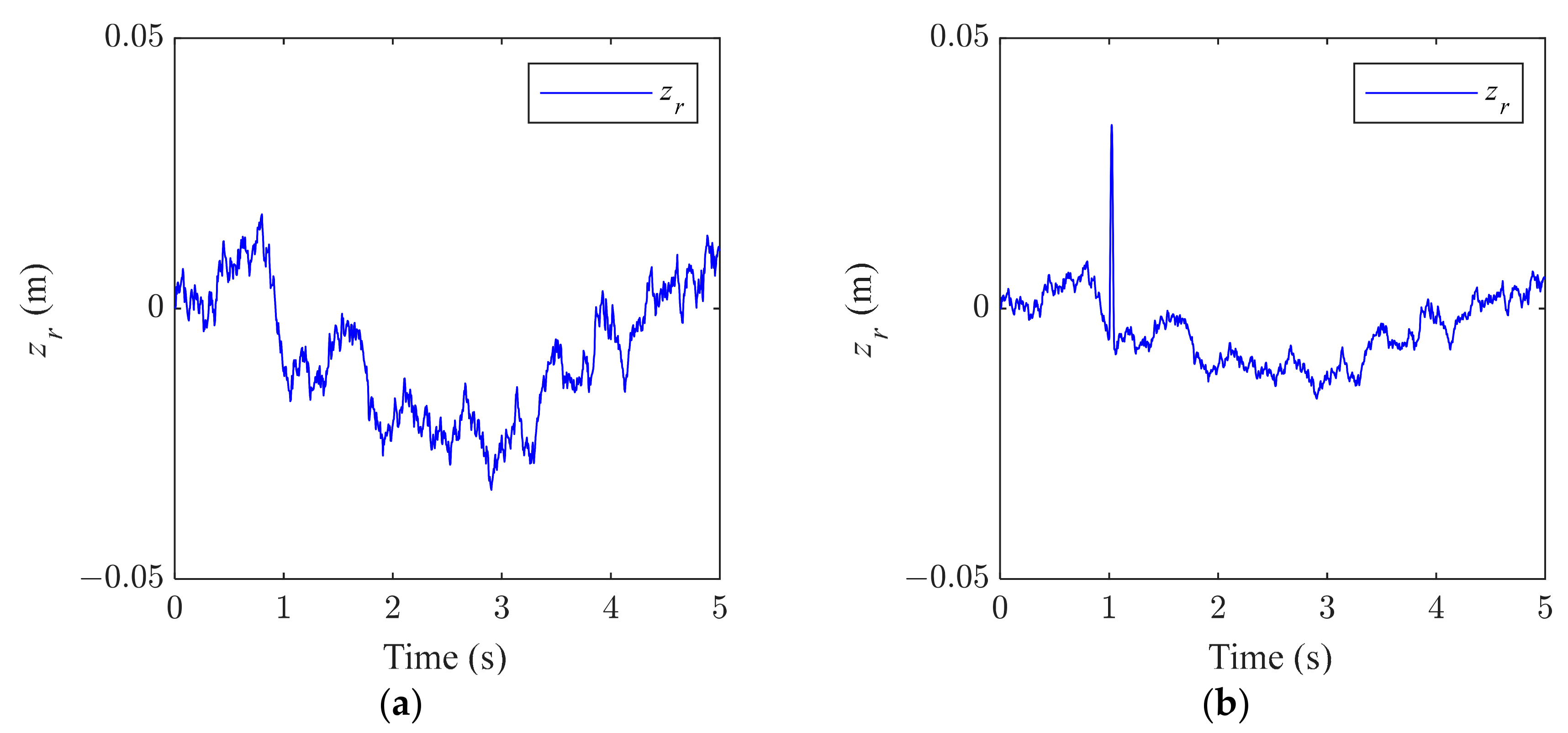
In order to verify the control effect of the designed robust control law on the suspension system, random road and pulse road surfaces were constructed as excitation inputs. The random pavement excitation takes the signal obtained with Gaussian white noise filtering as the input, as shown in Formula (49), which displays the time domain model of single-wheel pavement excitation where the pavement grade is defined as class C, as shown in Figure 6a. The pulse pavement excitation is composed of a speed bump and random pavement. The partial time domain model of random pavement has the same formula, Formula (49), and the pavement grade is defined as class B. The partial time domain model of the speed bump is given in Formula (50), as shown in Figure 6b.

$$\dot{z_r}\left(t\right)=-2\pi f_{min}{z}_r\left(t\right)+2\pi n_0\sqrt{G_q\left(n_0\right)V_{el}}w(t)$$

(49)

where $z_r\left(t\right)$ is the single wheel road excitation (m). $V_{el}$ is the vehicle speed (m/s) where the value is 8.33 m/s. t is time (s), $f_{min}=n_l{V}_{el}$, and $n_l$ is the lower limit of the pavement space cutoff frequency (0.011 m⁻¹). $w\left(t\right)$ is unit white noise. $n_0$ is the reference spatial frequency (0.1 m⁻¹). $G_q\left(n_0\right)$ is the road roughness coefficient (m³) and the value here is 256 × 10⁻⁶, which corresponds to class C pavement.

$$h\left(t\right)=\left\{\begin{array}{l}0 t\le 0 and t\ge 1+l_{bump}/V_{el}\\ \frac{h_{bump}}{2}\left(1-cos\frac{2\pi v}{l_{bump}}t\right) 1\le t\le 1+l_{bump}/V_{el}\end{array}\right.$$

(50)

where $h_{bump}$ refers to the speed bump section height, which is generally 0.04 m. $l_{bump}$ refers to the cross-section width of the speed bump, which is generally 0.40 m. t is time (s). $h\left(t\right)$ is the speed bump pulse excitation (m).

4.2. Result Analysis

To evaluate the effectiveness of the time-delay-dependent robust control, the suspension performance is compared under each time delay and fault combination. Uncertainty and fault are defined as follows. The perturbation uncertainty includes the perturbation of suspension stiffness and suspension foundation damping, defined as a sinusoidal change, where $f_k\left(t\right)=0.2\times \mathrm{s}\mathrm{i}\mathrm{n}\left(\mathrm{t}\right)$ and $f_c\left(t\right)=0.2\times \mathrm{s}\mathrm{i}\mathrm{n}\left(\mathrm{t}\right)$. The uncertainty with the time delay is set at three levels: T1 = 10 ms, T2 = 20 ms, and T3 = 35 ms. Three levels of gain fault are also set: F1 = 0.4, F2 = 0.6, and F3 = 0.8. There are nine kinds of combinations of each time delay and each fault. Simulation time is set as T_f = 5 s and the simulation step is set as T_s = 0.001 s to complete the simulation analysis. The results are shown in Figure 7, Figure 8, Figure 9, Figure 10, Figure 11 and Figure 12 and

Table 2. Class C random road excitation.

Group	Control	Performance Objective
		Body Acceleration P1 RMS (m/s2)	Wheel Acceleration P2 RMS (m/s2)	Suspension Dynamic Travel Displacement P3 RMS (m)
T1F1	TDI	0.6506	29.4023	0.0090
	TDD	0.5743 (↓11.73%)	18.1685 (↓38.21%)	0.0116 (↑28.89%)
T1F2	TDI	0.6910	22.4781	0.0081
	TDD	0.5455 (↓21.06%)	14.3002 (↓36.38%)	0.0091 (↑12.35%)
T1F3	TDI	0.7592	18.3505	0.0075
	TDD	0.5551 (↓26.88%)	12.3046 (↓32.95%)	0.0076 (↑1.33%)
T2F1	TDI	0.6042	21.6183	0.0098
	TDD	0.5653 (↓6.44%)	16.3878 (↓24.19%)	0.0117 (↑19.39%)
T2F2	TDI	0.6896	20.5215	0.0081
	TDD	0.5462 (↓20.79%)	13.4785 (↓34.32%)	0.0091 (↑12.35%)
T2F3	TDI	0.7815	18.3968	0.0075
	TDD	0.5606 (↓28.27%)	11.7127 (↓36.33%)	0.0076 (↑1.33%)
T3F1	TDI	0.6885	15.5796	0.0106
	TDD	0.5791 (↓15.89%)	14.9696 (↓3.92%)	0.0118 (↑11.32%)
T3F2	TDI	0.7344	14.1280	0.0078
	TDD	0.5647 (↓23.11%)	12.7440 (↓9.80%)	0.0090 (↑15.38%)
T3F3	TDI	0.8180	14.3193	0.0071
	TDD	0.5817 (↓28.89%)	11.3821 (↓20.51%)	0.0074 (↑4.23%)

and

Table 3. Pulse road excitation.

Group	Control	Performance Objective
		Body Acceleration P1 TDP (m/s2)	Wheel Acceleration P2 TDP (m/s2)	Suspension Dynamic Travel Displacement P3 TDP (m)
T1F1	TDI	5.8821	181.8380	0.0381
	TDD	5.2312 (↓11.07%)	188.9183 (↑3.89%)	0.0388 (↑1.84%)
T1F2	TDI	7.7457	173.6568	0.0315
	TDD	5.9154 (↓23.63%)	177.2359 (↑2.06%)	0.0340 (↑7.94%)
T1F3	TDI	9.0002	168.7068	0.0292
	TDD	6.4773 (↓28.03%)	164.9106 (↓2.25%)	0.0297 (↑1.71%)
T2F1	TDI	5.3118	185.2100	0.0375
	TDD	4.8198 (↓9.26%)	188.1241 (↑1.57%)	0.0392 (↑4.53%)
T2F2	TDI	7.0341	180.0214	0.0334
	TDD	5.7632 (↓18.07%)	173.3401 (↓3.71%)	0.0340 (↑1.80%)
T2F3	TDI	7.8919	175.6408	0.0289
	TDD	6.8615 (↓13.06%)	165.4193 (↓5.82%)	0.0297 (↑2.77%)
T3F1	TDI	5.3261	192.4663	0.0391
	TDD	5.2511 (↓1.41%)	190.4339 (↓1.06%)	0.0384 (↓1.79%)
T3F2	TDI	6.7472	188.3376	0.0372
	TDD	6.0080 (↓10.96%)	178.0504 (↓5.46%)	0.0328 (↓11.83%)
T3F3	TDI	7.6170	183.5802	0.0335
	TDD	6.8469 (↓10.11%)	166.8327 (↓9.12%)	0.0288 (↓14.03%)

, where “↑” represents an increase and “↓” represents a decrease.

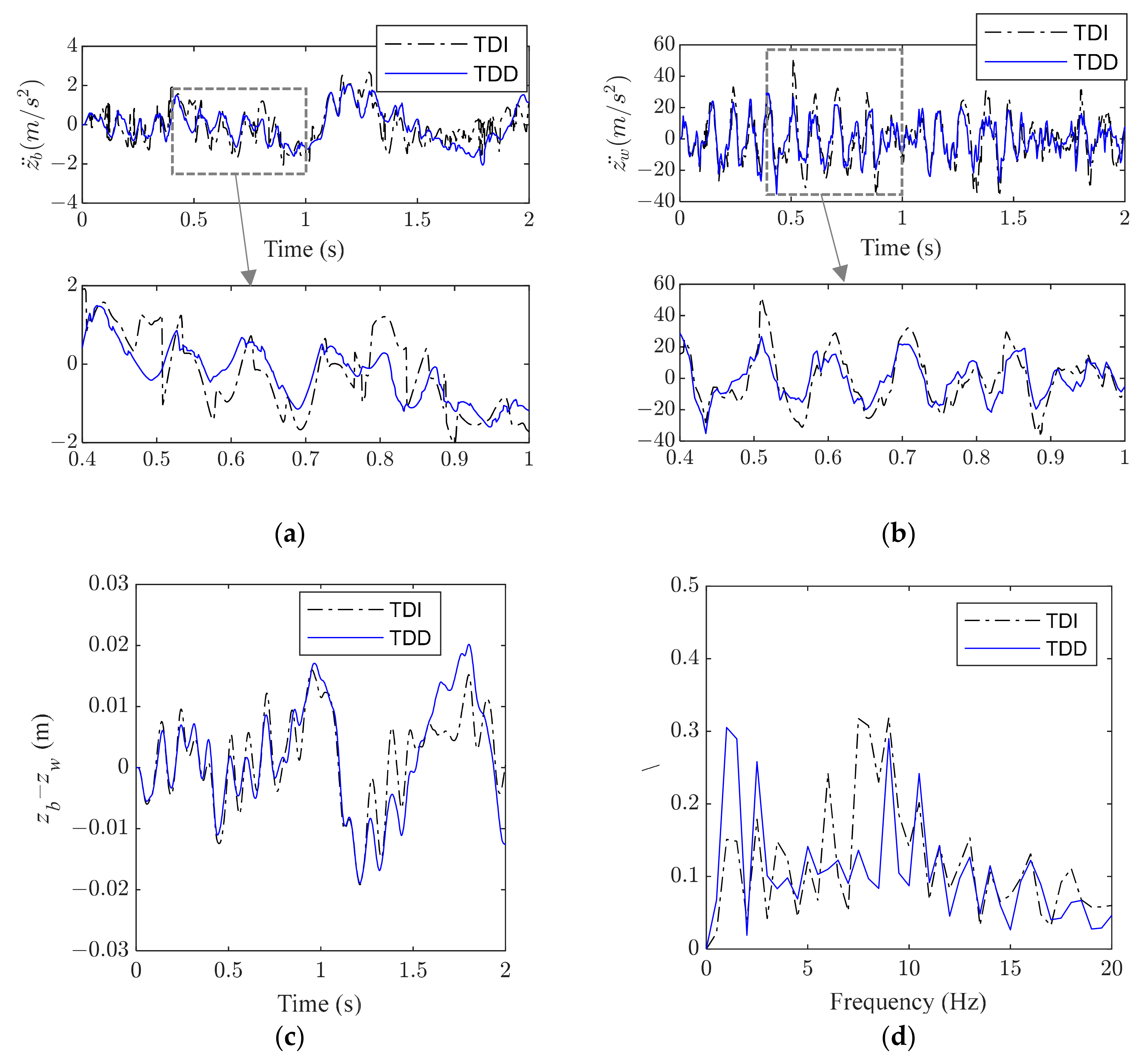
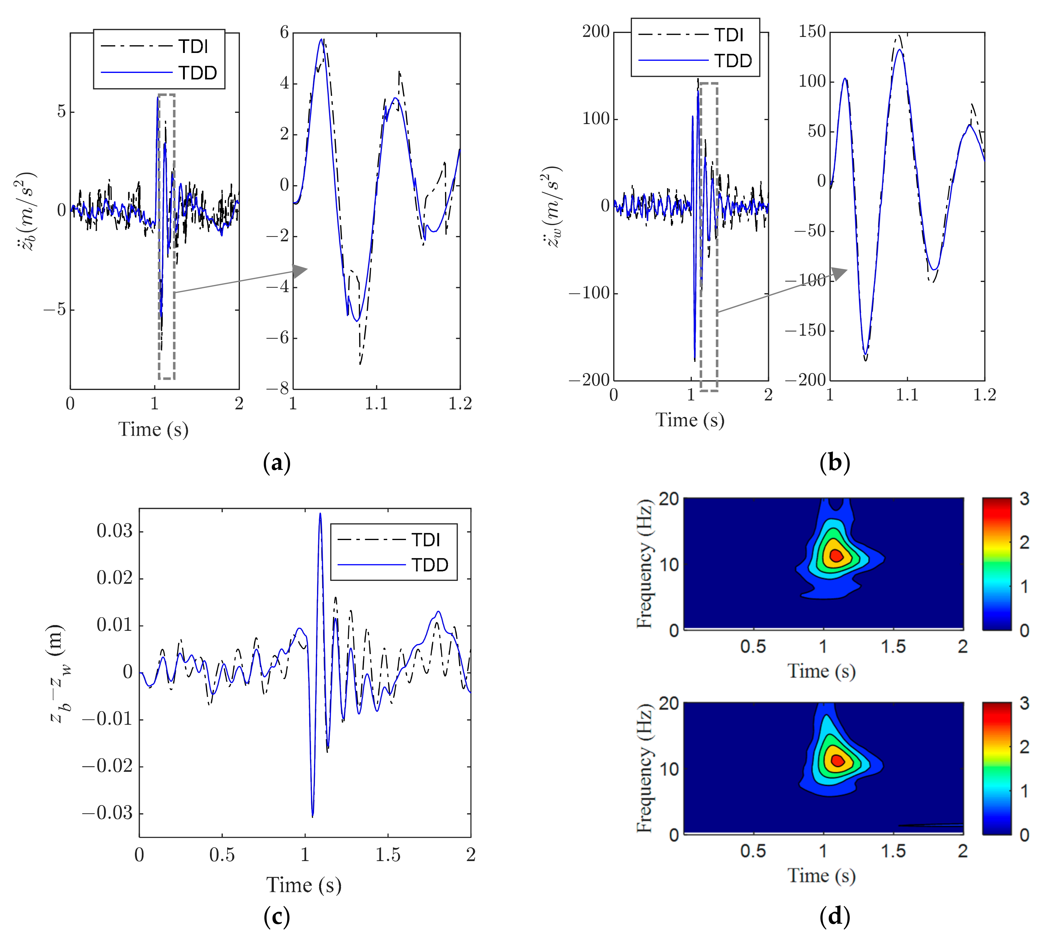
Taking the simulation results of the T2F2 combination (time delay is 20 ms and the fault is 0.6) as an example, 0–2 s data were taken to analyze and explain the three key performance objectives of suspension (body acceleration, wheel acceleration, and suspension dynamic travel displacement), as shown in Figure 7, Figure 8, Figure 9 and Figure 10. Figure 7 and Figure 8 shows class C random road excitation. It can be seen from the local magnification of vehicle acceleration in the time domain that TDD control under random road excitation is significantly reduced compared with TDI control. At the same time, TDI control and TDD control also increase and decrease in the range of 0–20 Hz in the frequency domain diagram of vehicle body acceleration and, in general, TDD control is slightly better, as shown in Figure 7d. Compared with TDI control, the wheel acceleration of the corresponding period is also significantly reduced under TDD control and the dynamic travel time of the suspension is increased to a certain extent. However, the dynamic travel time under the random class C road surface is controlled within 0.025 m (group T2F2). The random road excitation input is an approximately stationary state, with specific random distribution characteristics according to the graph data. 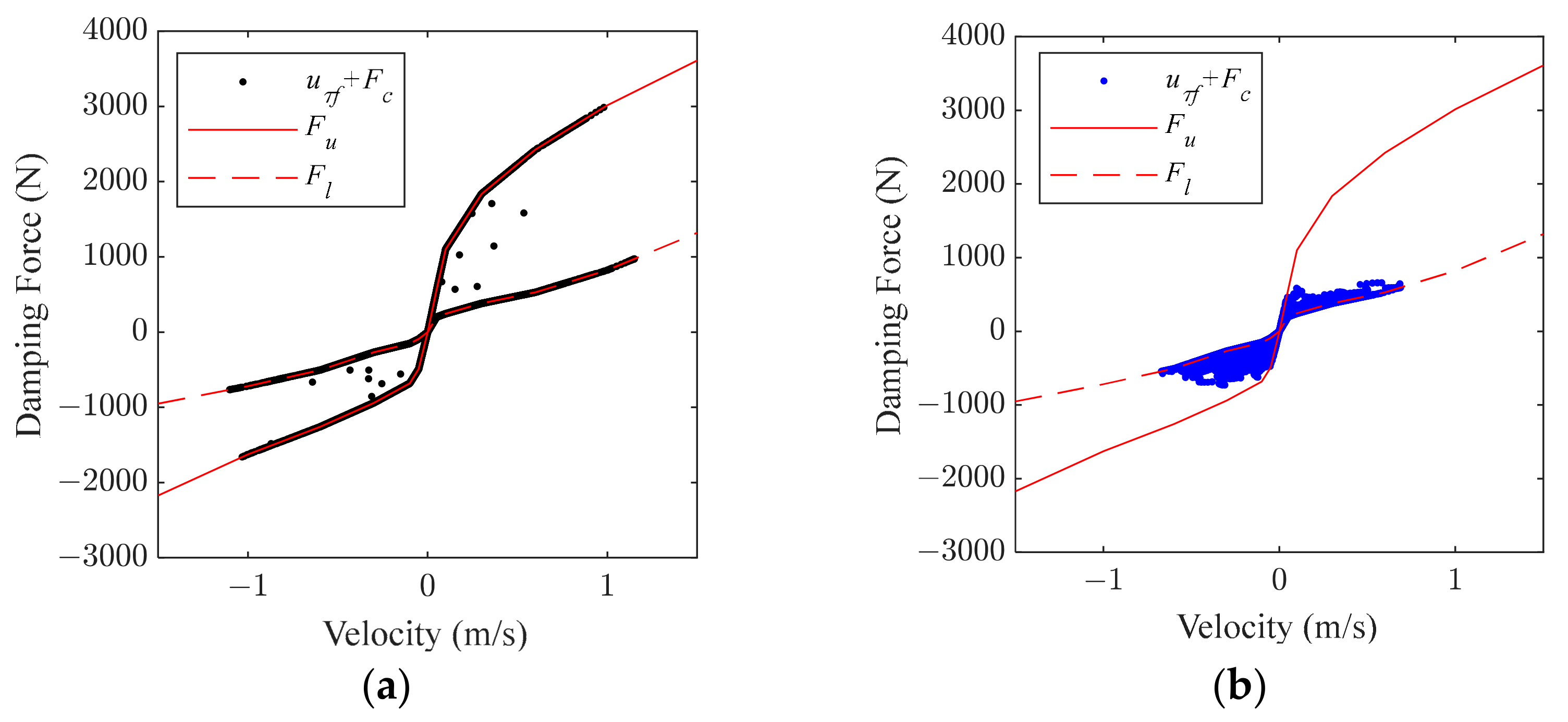In this approximately stationary case, the difference in the control effect with or without time delay consideration can be further characterized by the quantized root mean square value difference, as shown in Table 2. In addition, it can be seen from Figure 8a,b that both TDI and TDD control forces are within the constraint boundaries shown in Formula (2). The definitions of $F_c$, $F_u$, and $F_l$ are shown in Formula (51).

$$\left\{\begin{array}{c}{F}_c=c_s\left({\dot{z}}_b\left(t\right)-{\dot{z}}_w\left(t\right)\right)\\ F_u=c_{max}\left({\dot{z}}_b\left(t\right)-{\dot{z}}_w\left(t\right)\right)\\ F_l=c_{min}\left({\dot{z}}_b\left(t\right)-{\dot{z}}_w\left(t\right)\right)\end{array}\right.$$

(51)

In Figure 9 and Figure 10, the results for pulse road excitation are shown. According to the time domain partial amplification of vehicle body acceleration, TDD control under pulse road excitation is superior to TDI control, which is reflected in both the time domain peak value and the speed of vibration attenuation. At the same time, the area size of each color block of TDI control and TDD control in the time–frequency domain diagram of vehicle body acceleration can also represent this advantageous feature (the smaller the area of one color, the lower the vibration intensity, that is, the better the control effect), as shown in Figure 9d.

Compared with TDI control, the wheel acceleration of the corresponding period is slightly reduced by TDD control and the suspension dynamic travel displacement is slightly increased but this increase is slight. The input energy of pulse pavement excitation is significant and the state is non-stationary. The mutation time is short, far less than the critical delay, and the mutation amount is significant. In the case of this large, transient, and abrupt change, the difference in control effect with and without a delay can be further characterized by the difference in the quantified time domain peak value, as shown in Table 3. In addition, it can be seen from Figure 10a,b that both TDI and TDD controlling forces are within the constraint boundaries shown in Formula (2).

The statistics of each quantitative evaluation index are shown in Table 2 and Table 3. Table 2 shows the statistics of random class C pavement excitation input data. Under the condition that the road excitation energy is small and approximately stable, the root mean square (RMS) value of wheel acceleration under different combinations of uncertainty and faults shows that with the increase in time delay, the control effect of TDD control gradually becomes superior to that of TDI control. The maximum change is −28.89% (group T3F3) and the root mean square value of body acceleration also decreases significantly. However, due to the mutual restriction relationship between the three suspension performance variables, the root mean square value of dynamic travel time increases with a maximum variation of 28.89% (group T1F1). However, the maximum suspension dynamic travel displacement at this time is about 0.030 m (group T1F1), far less than the maximum suspension travel time of 0.080 m. Table 3 shows the input data statistics of pulse pavement excitation. Under the condition that the road excitation energy is significant and non-stationary, the time domain peak (TDP) value of body acceleration under an instantaneous and significant change and different combinations of uncertainty and faults shows that TDD control is superior to TDI control. The maximum variation is −28.03% and the peak value of wheel acceleration in the time domain and the peak value of dynamic travel time in the time domain only slightly increase. The variation is less than 7.94%.

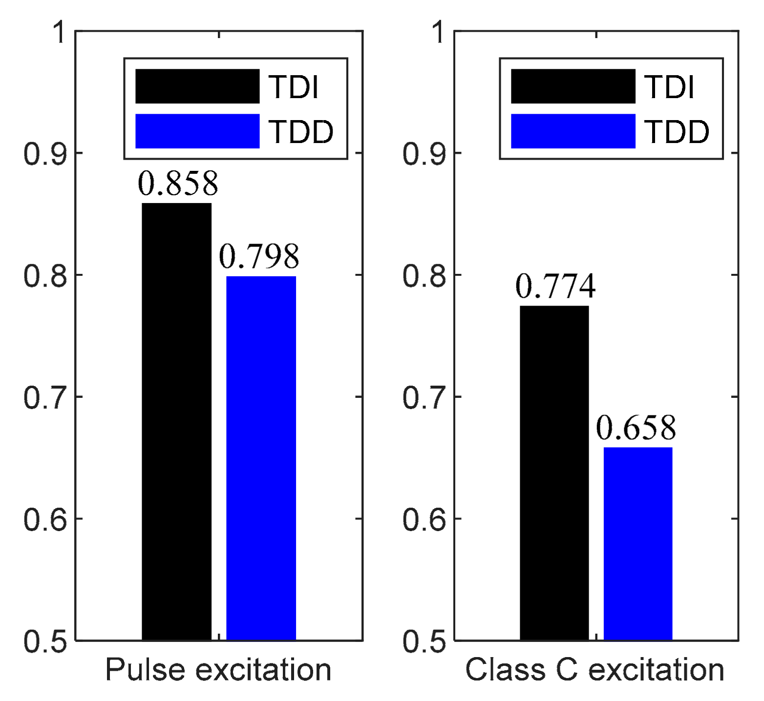
Furthermore, in order to compare the comprehensive effect of TDI control and TDD control, assuming that the probability of occurrence of each combination state is the same, the normalized arithmetic average of each index of each combination is obtained, as shown in Figure 11a,b. The wheel acceleration under class C random road excitation shows that TDD is superior to TDI control while the suspension dynamic travel displacement increases. Under pulse road excitation, the body acceleration, wheel acceleration, and suspension dynamic travel displacement are improved in TDD control compared with TDI control. Based on the weighting coefficient defined in Section 2, a comprehensive evaluation index is obtained by weighted summating the three key suspension performance variables, as shown in Figure 12. The results show that compared with TDI control, the comprehensive index of TDD control is improved by 14.99% under class C random road excitation and the comprehensive index of TDD is improved by 6.99% under pulse road excitation.

5. Discussion and Conclusions

A time-delay-dependent (TTD) robust control strategy is designed for V-CSS’s uncertainty, fault, and input time delay. It is based on a robust control to ensure the dynamic performance and stability of the system. It can prevent the time delay caused by fault diagnosis and control law recombination. In this study, a normalized arithmetic average weighted comprehensive index of the three key performance objectives of the suspension system, namely body acceleration, wheel acceleration, and suspension dynamic travel displacement, is constructed to evaluate the control effect. Nine uncertainty and fault combinations are used for simulation and comparison with a time-delay-independent (TDI) control under approximate stationary and non-stationary road excitation, respectively. The results show that the comprehensive evaluation effect of the proposed TDD control is superior to that of the TDI control and that an improvement in the control effect of 14.99% could be achieved under approximate stationary excitation, while an improvement of 6.99% was seen under non-stationary excitation. In this article, the two degrees of freedom vehicle suspension model only involves a set of execution units and the robust control concept is used to ensure its feasibility and effectiveness. Although a series of comparative simulations demonstrated the feasibility and effectiveness of the proposed control, the following limitations are worth investigating in the future: (1) the model could be extended to the entire vehicle model, taking into account the synergistic effect of four groups of execution units, ensuring overall performance; (2) although the designed TDD control provides a more concise structure, conservation minimization of control methods was not extensively explored in this study and could be the object of future studies; and (3) data-driven methods and robust fusion control could be introduced into future research, integrating the advantages of both methods to fully utilize system data for fast convergence and the signal estimation problem.