Configuration Optimization of a Shell-and-Tube Heat Exchanger with Segmental Baffles Based on Combination of NSGAII and MOPSO Embedded Grouping Cooperative Coevolution Strategy

Abstract

A design indicators prediction model using the Bell-Delaware method for a shell-and-tube heat exchanger with segmental baffles (STHX-SB) is constructed and validated by experiment. The average errors of heat transfer capacity and tube-side pressure drop are 8.52% and 7.92%, respectively, and the predicted weight is the same as the weight obtained by Solidworks commercial software, which indicates the model’s reliability. Parametric influences of the outside diameter of the heat dissipation tube, clearance between heat dissipation tubes, heat dissipation tube length, and tube bundle bypass flow clearance on heat transfer capacity per tube-side pressure drop and heat transfer capacity per weight are studied, and it indicates that whether the interaction between factors is considered or not, both heat transfer capacity per tube-side pressure drop and heat transfer capacity per weight are the most sensitive to outside diameter of heat dissipation tube and the least sensitive to heat dissipation tube length based on the Sobol’ method. To avoid falling into local optima due to algorithm convergence being too fast and to improve the reliability of solving complex optimization problems, Non-Dominated Sorted Genetic Algorithm II (NSGAII) and Multi-Objective Particle Swarm Optimization (MOPSO) embedded grouping cooperative coevolution (NSGAII-MOPSO-GCC) is proposed to optimize the studied four configuration parameters to maximize heat transfer capacity per tube-side pressure drop and heat transfer capacity per weight for STHX-SB, simultaneously. Compared with the original structure, heat transfer capacity per tube-side pressure drop and heat transfer capacity per weight of the chosen solutions separately increased by 57.66% and 4.63%, averagely, and in the optimization comparison of NSGAII, MOPSO, and NSGAII-MOPSO-GCC, NSGAII-MOPSO-GCC has the best performance, which shows that the proposed method is effective and feasible and can supply beneficial solutions and valuable guidance for heat exchanger design and improvement.

1. Introduction

As widely used mechanical devices in various kinds of industrial fields like aerospace, automotive, food, chemical, energy, and so on, heat exchangers have the ability to transfer heat from the fluid of lower temperature to the fluid of higher temperature [1,2]. As heat exchangers have the advantages of high efficiency and reliability, they are frequently adopted in lubricating oil systems in aero-engines to heat fuel and cool lubricating oil simultaneously, which can improve fuel combustion efficiency, prevent fuel from freezing, ensure sufficient cooling of bearings, and guarantee smooth low-temperature cold start of aero-engines. Therefore, pursuing comprehensive high performance for heat exchangers is meaningful and significant in engineering applications [3], and thus numerous studies on heat exchanger configuration optimization have been conducted.

The traditional optimization design of heat exchangers is mainly through gradually changing configuration parameters to meet the requirements of both designers and users in iterative design processes. Although using this research and development process could ultimately achieve the optimization goal, it consumes a lot of costs and time, and may not ultimately lead to a particularly excellent design solution. As various optimization algorithms have been developed well in these years, using optimization algorithms to achieve optimal design of heat exchangers for better characteristic indicators has been increasingly widely used, and its effectiveness and applicability have been increasingly recognized by many researchers. Up to now, in terms of optimization design of heat exchangers, good results have been achieved by adopting many classic and newly developed optimization algorithms, like Non-Dominated Sorted Genetic Algorithm II (NSGAII) [4,5], Multi-Objective Particle Swarm Optimization (MOPSO) [6], Taguchi approach [7], Differential Evolution (DE) [8], Falcon Optimization Algorithm (FOA) [9], Jaya [10], Topology optimization [11], and so on. In the research of Seema Singh et al. [12], three classic optimization algorithms and three newly developed optimization algorithms were adopted to optimize plate and frame heat exchanger structural parameters. There are two kinds of studies that can be divided based on the existing studies on heat exchanger design optimization using optimization algorithms: combining optimization algorithms and theoretical analysis, and combining optimization algorithms and numerical simulation.

In terms of combining optimization algorithms and theoretical analysis, parameters optimization was conducted by Yayun Zhang et al. [13] using Genetic Algorithm based on the proposed function models for a rectangular staggered fins heat exchanger. Vidyadhar H. Iyer et al. [14] proposed the Adaptive Range Genetic Algorithm to optimize a shell-and-tube heat exchanger in the aspects of design and economy based on theoretical design calculation. An optimization strategy of combining genetic algorithm with entransy theory was proposed by Jian wen et al. [15] to realize configuration optimization for a shell-and-tube heat exchanger with helical baffles. In the research of Hongyoung Lim et al. [16], for mobile air conditioning systems, a strategy of replacing a louver fin heat exchanger by one kind of bare tube heat exchanger as an evaporator was proposed, and the approximated assisted optimization method was adopted to optimize five independent design variables of bare tube heat exchanger based on theoretical calculation.

In terms of combining optimization algorithms and numerical simulation, for shell-and-tube heat exchangers with helical baffles, Jian Wen et al. [17] and Simin Wang et al. [18,19] both conducted numerical simulation to analyze performances, and obtained corresponding response surface functions for different structural parameters. Then, structural parameters multi-objective optimization was conducted using Genetic Algorithm. Moreover, a spiral-wound heat exchanger was also optimized by Simin Wang et al. [20] through applying this method. In the research of Xinting Wang et al. [21], numerical simulation was conducted for shell-and-tube heat exchangers separately with segmental baffles, continuous helical baffles, and staggered baffles to study their performances, and shell-and-tube heat exchanger with staggered baffles was chosen to be the one that has the best comprehensive performance through comparison. Then, Genetic Algorithm combining with artificial neural network was used to optimize the selected heat exchanger to pursue comprehensive optimum heat transfer rate and pressure drop. Paweł Ocłoń et al. [22] optimized high-temperature fin-and-tube heat exchanger manifold shape using Particle Swarm Optimization and Continuous Genetic Algorithms based on numerical simulation. Hadi Keramati et al. [23] utilized Deep Reinforcement Learning and Boundary Representation combined with numerical simulation to optimize heat exchanger shape to enhance heat transfer and suppress flow resistance. In the research of Kizhakke Kodakkattu Saijal et al. [24], Genetic Algorithm was adopted to pursue heat transfer rate maximizing and pressure drop minimizing based on numerical simulation analysis. Finally, heat transfer rate per pressure drop was utilized as one criterion to find a satisfactory optimization result. In the research of Chuangeng Tang et al. [25], two new cross-flow radiator structures were designed through Topology optimization, with the objective function aimed at achieving the minimum temperature difference and pressure drop. The influence of six channel heights was analyzed using the evaluation criterion Colbum coefficient per friction factor to obtain the result with the best heat dissipation ability.

Even though there already exist many studies about heat exchanger performance improvement, most of the researched heat exchangers are large-sized. Meanwhile, due to the light weight and few space occupation design requirements for airborne equipment, the heat exchangers adopted in aero-engines are usually small-sized, and their comprehensive high-performance design needs to be researched more. Thus, in this research, in order to provide a stable design theory base and promote engineering application for heat exchangers in the aerospace field, a small-sized shell-and-tube heat exchanger with segmental baffles (STHX-SB), which has been widely utilized in aero-engines, was studied. One design indicators prediction model adopting the Bell–Delaware method was constructed and validated by experiment. The influences of four structure parameters, which are significant in engineering applications, on design indicators were studied, and their global sensitivity indices were analyzed based on Sobol’ method to reveal influential degrees. Then, in order to avoid falling into local optima due to algorithm convergence being too fast and to improve the reliability of solving complex optimization problem, based on the above research, one combination optimization method of NSGAII and MOPSO embedded grouping cooperative coevolution was proposed to optimize the analyzed four key configuration parameters to improve comprehensive performance for STHX-SB, which can provide beneficial solutions and valuable guidance for heat exchanger design and improvement.

2. Design Indicators Prediction Model Construction

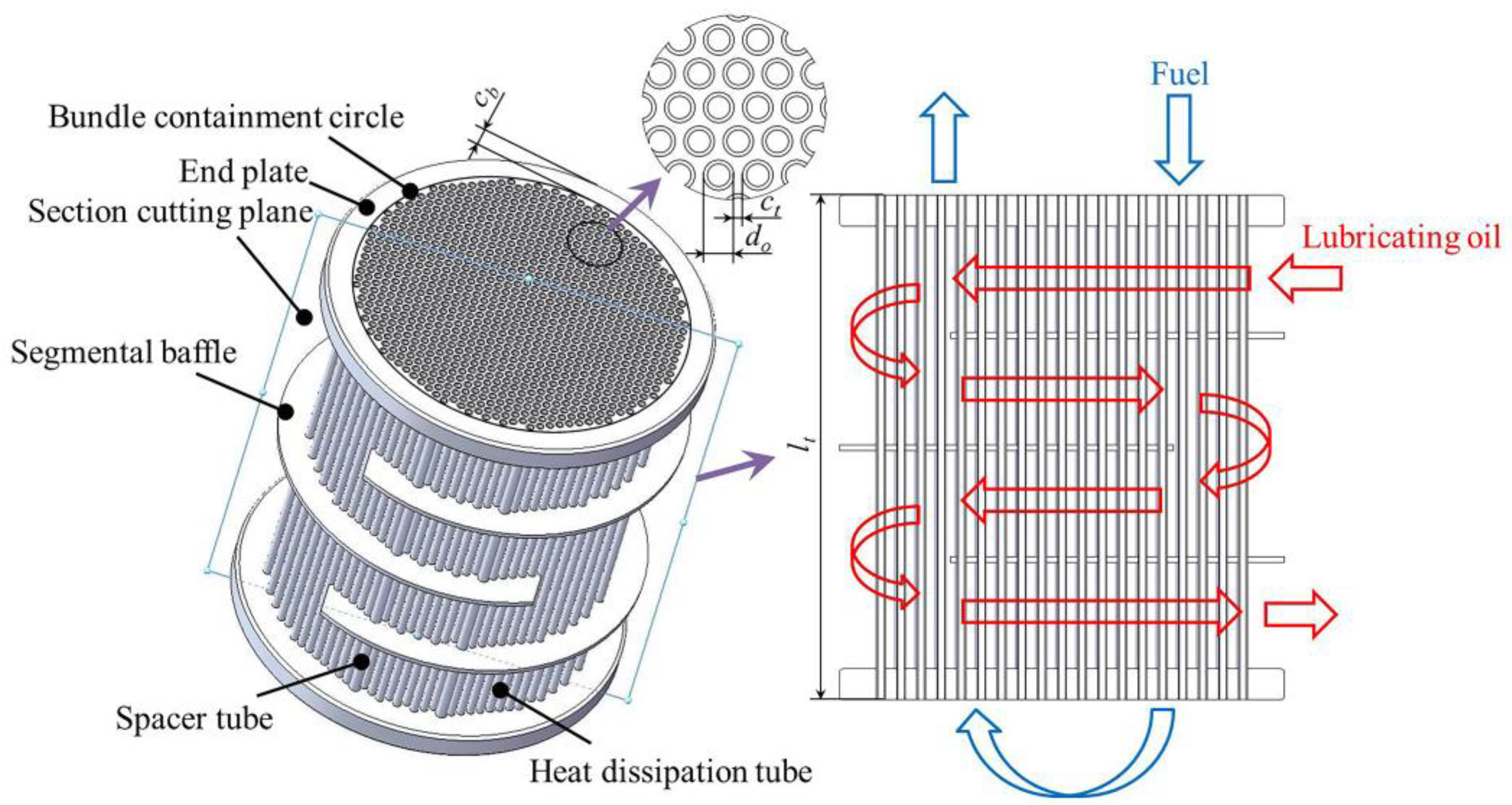
2.1. STHX-SB Structure Description

STHX-SB studied in this research is one kind of heat exchanger that is adopted in one turbine-shaft aero-engine to heat cold fuel by hot lubricating oil, which is smaller, lighter, and more compact compared with heat exchangers in many other industrial fields. STHX-SB is mainly composed of heat dissipation tubes, end plates, segmental baffles, and spacer tubes. In STHX-SB, uniformly distributed segmental baffles are located by spacer tubes, and two end plates are fixed with heat dissipation tubes ends. As shown in Figure 1, hot lubricating oil cross flows through outside heat dissipation tubes and cold fuel flows inside them, and then heat exchange can be realized between two fluids through tubes wall. The materials of heat exchanger, hot side fluid, and cold side fluid are aluminum alloy, lubricating oil 4050 [26], and fuel RP-3 [27], respectively. Main structural parameters and normal working conditions of STHX-SB are presented in

Table 1. Structural parameters of STHX-SB.

Parameter	Value
Outside diameter of heat dissipation tube do	2.36 mm
Clearance between heat dissipation tubes ct	0.64 mm
Heat dissipation tube length lt	130 mm
Tube bundle bypass flow clearance cb	7.5 mm
Baffle cut Pc	0.25
Baffles number Nb	3
Baffle diameter db	115 mm
Baffle thickness tb	1.5 mm
End plates number Np	2
Thickness of end plate tp	8 mm
Spacer tube number between baffles Ns_b	4
Wall thickness of spacer tube ts_w	0.305 mm
Wall thickness of heat dissipation tube tt_w	0.305 mm
Shell passes number Zs	1
Tube passes number Zt	2
Shell/Tube-side inlet/outlet diameter DN	20 mm

and

Table 2. STHX-SB normal working conditions.

Working Condition	Value
Flow rate of lubricating oil qo	15 L/min
Inlet temperature of lubricating oil To	383 K
Fuel flow rate qf	6 L/min
Fuel inlet temperature Tf	333 K

, separately.

2.2. Design Indicators Calculation Model

2.2.1. Computation Equations

In engineering applications, heat exchanger efficiency and economy are two significant considerations. Thus, heat transfer capacity per tube-side pressure drop Q/ΔP and heat transfer capacity per weight Q/G are two main indicators in STHX-SB configuration design. The higher these two design indicators, the better the comprehensive performance looks. Before predicting Q/ΔP and Q/G, Q, ΔP, and G need to be computed reliably. In this research, ε-NTU relational expression and the Bell–Delaware method [28] were adopted in Q calculation, and the computation equations of Q, ΔP, and G are presented in

Table 3. Computation equations for heat transfer capacity [28,29,30,31,32,33,34].

Parameter	Equation	No.
Heat transfer capacity	$Q=\epsilon W_{\min }(t_1-t_2)$	(1)
Heat transfer efficiency	$\epsilon =\frac{2}{1+C^{\ast }+\sqrt{1+C^{\ast }{}^2}(1+e^{-NTU\sqrt{1+C^{\ast }{}^2}})/(1-e^{-NTU\sqrt{1+C^{\ast }{}^2}})}$	(2)
Heat capacity ratio	$C^{\ast }=W_{\min }/W_{\max }$	(3)
Number of transfer units	$NTU=\frac{KA}{W_{\min }}$	(4)
Total heat transfer coefficient	$K=\frac{{\alpha }_o{\alpha }_i}{{\alpha }_o+{\alpha }_i}$	(5)
Heat transfer coefficient of tube-side	${\alpha }_i=0.027\frac{{\lambda }_i}{d_i}{\mathrm{Re}}_i^{0.8}{\mathrm{Pr}}_i{}^{1/3}{(\frac{{\mu }_i}{{\mu }_{iw}})}^{0.14}$ $({\mathrm{Re}}_i>\mathrm{10,000},0.7<{\mathrm{Pr}}_i<\mathrm{16,700},l_t/d_i\ge 60)$, ${\alpha }_i=0.027(1-\frac{6\times {10}^5}{{\mathrm{Re}}_i^{1.8}})\frac{{\lambda }_i}{d_i}{\mathrm{Re}}_i^{0.8}{\mathrm{Pr}}_i{}^{1/3}{(\frac{{\mu }_i}{{\mu }_{iw}})}^{0.14}$ $(2300\le {\mathrm{Re}}_i\le \mathrm{10,000},0.7<{\mathrm{Pr}}_i<\mathrm{16,700},l_t/d_i\ge 60)$, ${\alpha }_i=1.86\frac{{\lambda }_i}{d_i}{({\mathrm{Re}}_i{\mathrm{Pr}}_i\frac{d_i}{l_t})}^{1/3}{(\frac{{\mu }_i}{{\mu }_{iw}})}^{0.14}$ $({\mathrm{Re}}_i<2300,0.6<{\mathrm{Pr}}_i<6700,{\mathrm{Re}}_i{\mathrm{Pr}}_i{l}_t/d_i\ge 100)$.	(6)
Heat transfer coefficient of shell-side	${\alpha }_o={\alpha }_{oid}{J}_c{J}_l{J}_b{J}_s{J}_r$	(7)
Baffle layout correction factor	$\left\{\begin{array}{l}{J}_c=0.55+0.72F_c\hfill \\ F_c=1-\frac{{\theta }_{ctl}}{\pi }+\frac{\sin {\theta }_{ctl}}{\pi }\hfill \\ {\theta }_{ctl}=2{\cos }^{-1}(\frac{D_s-2l_c}{D_{ctl}})\hfill \\ D_{ctl}=D_{otl}-d_o\hfill \end{array}\right.$	(8)
Baffle leakage effect correction factor	$\left\{\begin{array}{l}{J}_l=0.44(1-r_s)+[1-0.44(1-r_s)]e^{-2.2r_{lm}}\hfill \\ r_s=\frac{A_{o,sb}}{A_{o,sb}+A_{o,tb}}\hfill \\ r_{lm}=\frac{A_{o,sb}+A_{o,tb}}{A_{o,cr}}\hfill \end{array}\right.$	(9)
Tube bundle bypass correction factor	$\left\{\begin{array}{l}{J}_b=\left\{\begin{array}{ll}1,\hfill & N_{ss}^{+}\ge 0.5\hfill \\ e^{-C{r}_b[1-{(2N_{ss}^{+})}^{\frac{1}{3}}]},\hfill & N_{ss}^{+}\le 0.5\hfill \end{array}\right.\hfill \\ C=\left\{\begin{array}{ll}1.35,\hfill & {\mathrm{Re}}_o\le 100\hfill \\ 1.25,\hfill & {\mathrm{Re}}_o>100\hfill \end{array}\right.\hfill \\ r_b=\frac{A_{o,bp}}{A_{o,cr}}\hfill \\ N_{ss}^{+}=\frac{N_{ss}}{N_{r,cc}}\hfill \\ N_{r,cc}=\frac{D_s-2l_c}{X_l}\hfill \end{array}\right.$	(10)
Correction factor for unequal span heat transfer	$\left\{\begin{array}{l}{J}_s=\frac{N_b-1+{(L_i^{+})}^{(1-n)}+{(L_o^{+})}^{(1-n)}}{N_b-1+L_i^{+}+L_o^{+}}\hfill \\ L_i^{+}=\frac{L_{b,i}}{L_{bc}}\hfill \\ L_o^{+}=\frac{L_{b,o}}{L_{bc}}\hfill \\ n=\left\{\begin{array}{ll}0.6,\hfill & {\mathrm{Re}}_o\ge 1000\hfill \\ 1/3,\hfill & {\mathrm{Re}}_o<1000\hfill \end{array}\right.\hfill \end{array}\right.$	(11)
Temperature gradient correction factor	$\left\{\begin{array}{l}{J}_r=\left\{\begin{array}{ll}1,\hfill & {\mathrm{Re}}_o\ge 100\hfill \\ \mathrm{linear} \mathrm{interpolation},\hfill & 20<{\mathrm{Re}}_o<100\hfill \\ {(10/N_{r,c})}^{0.18},\hfill & {\mathrm{Re}}_o\le 20\hfill \end{array}\right.\hfill \\ N_{r,c}=N_{r,cc}+N_{r,cw}\hfill \end{array}\right.$	(12)

,

Table 4. Computation equations for tube-side pressure drop [28,29,30,31,32,33,34].

Parameter	Equation	No.
Tube-side pressure drop	$\Delta P=\Delta P_i+\Delta P_r+\Delta P_N$	(13)
On-way resistance	$\Delta P_i=\left\{\begin{array}{ll}\frac{64}{{\mathrm{Re}}_i}{Z}_t\frac{l_t}{d_i}\frac{{\rho }_i{u}_i^2}{2}{(\frac{{\mu }_i}{{\mu }_{iw}})}^{-0.25},\hfill & {\mathrm{Re}}_i<2000\hfill \\ (0.014+1.56{\mathrm{Re}}_i^{-0.42})Z_t\frac{l_t}{d_i}\frac{{\rho }_i{u}_i^2}{2}{(\frac{{\mu }_i}{{\mu }_{iw}})}^{-0.14},\hfill & {\mathrm{Re}}_i\ge 2000\hfill \end{array}\right.$	(14)
Elbow flow resistance	$\Delta P_r=4\frac{{\rho }_i{u}_i^2}{2}{Z}_t$	(15)
Inlet and outlet flow resistance	$\Delta P_N=1.5\frac{{\rho }_i{u}_N^2}{2}$	(16)

and

Table 5. Computation equations for weight.

Parameter	Equation	No.
Weight	$G=G_p+G_b+G_t+G_s$	(17)
Weight of end plates	$G_p=0.25\pi (d_b^2-N_t{d}_o^2)t_p{N}_p{\rho }_{al}\cdot {10}^{-9}$	(18)
Weight of baffles	$\begin{array}{l}{G}_b=\left\{[0.25\pi -0.25\arccos (1-2P_c)+(0.5-P_c)\sqrt{P_c(1-P_c)}]d_b^2\right.\\ \begin{array}{cc}& \end{array}\left.-0.25\pi d_o^2(N_t-N_{t\_cut})\right\}{t}_b{N}_b{\rho }_{al}\cdot {10}^{-9}\end{array}$	(19)
Weight of heat dissipation tubes	$G_t=0.25\pi l_t(d_o^2-d_i^2)N_t{\rho }_{al}\cdot {10}^{-9}$	(20)
Weight of spacer tubes	$G_s=\pi (l_t-t_p{N}_p-t_b{N}_b)t_{s\_w}(d_o+t_{s\_w})N_{s\_b}{\rho }_{al}\cdot {10}^{-9}$	(21)

, respectively.

2.2.2. Model Calculation Process

As temperature is changing with the flowing of fluid, fluid physical properties are not constant in the heat exchanger. In order to consider this influence in calculation, fluid average temperature was computed by arithmetic mean of inlet and outlet temperatures, and heat dissipation tube wall temperature was computed by arithmetic mean of fluid temperatures of two sides. Meanwhile, outlet temperatures were not known before starting computation. Hence, in this research, one strategy of assuming heat transfer capacity and repeatedly correcting it through iterative calculation was utilized to calculate Q. The design indicators prediction model calculation process is depicted as follows:

(1)

Define heat exchanger working conditions and configuration parameters.

(2)

Q calculation.

(a)

Assume STHX-SB heat transfer capacity Q_as.

(b)

Compute fuel average temperature T_{f_ave}, lubricating oil average temperature T_{o_ave}, and heat dissipation tube wall temperature T_{t_w} by Equations (22)–(24). In these equations, W_f and W_o are under the inlet temperatures of fuel and lubricating oil, respectively.

$$T_{f\_ave}=T_f+\frac{Q_{as}}{2W_f},$$

(22)

$$T_{o\_ave}=T_o-\frac{Q_{as}}{2W_o},$$

(23)

$$T_{t\_w}=\frac{T_{f\_ave}+T_{o\_ave}}{2},$$

(24)

(c)

Compute heat transfer capacity Q by Equations (1)–(12). Unless otherwise required, the physical properties of fuel and lubricating oil are defaulted to the values under T_{f_ave} and T_{o_ave}, respectively.

(d)

If Q can fulfill the requirement depicted by Equation (25), output Q, otherwise utilize the computed Q in this iteration as Q_as in the next iteration and recompute from Step (b). Error E was set as 0.05 kW in this study.

$$\left|Q-Q_{as}\right|\le E,$$

(25)

(3)

Compute ΔP by Equations (13)–(16). Unless otherwise required, fuel physical properties are defaulted to the values under T_{f_ave}.

(4)

Compute and output weight G by Equations (17)–(21).

It needs to be noted that in order to make calculation convenient, there are some simplifying assumptions of the calculation model: (1) the fluids in the heat exchanger are considered in steady state; (2) the default properties of fluids and solid are under average temperatures computed by Equations (22)–(24); (3) the radiative heat dissipation from heat exchanger to environment is neglected; (4) the heat exchanger is assumed to be new and free of dirt inside.

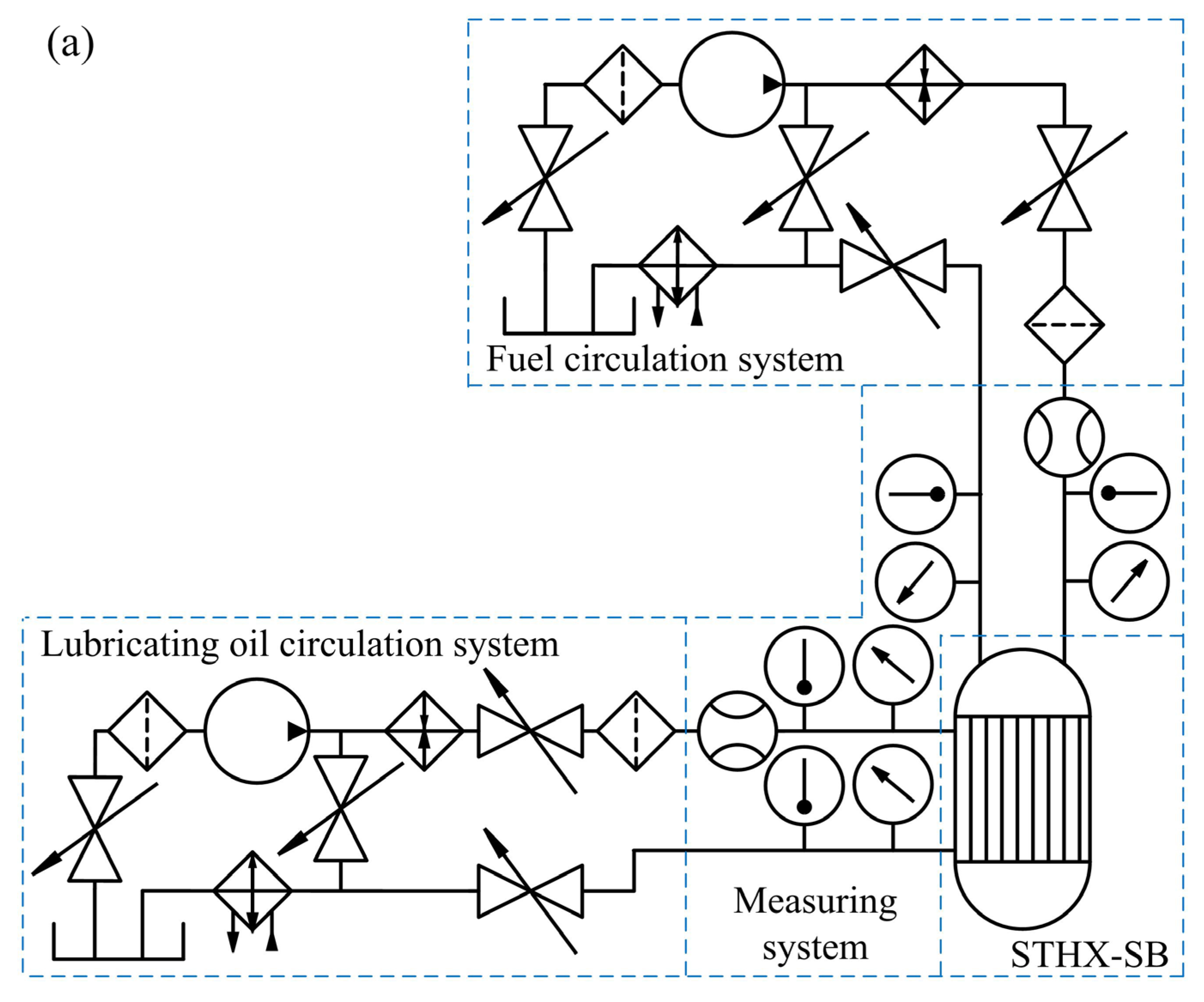
2.3. Experimental Verification

A thermodynamic characteristic and flow resistance experiment was conducted to verify the proposed model reliability. In this experiment, flow rate and inlet temperature of lubricating oil and flow rate of fuel as shown in Table 2 were used as constant operating conditions, and inlet temperature of fuel was changed from 318 K to 348 K with a changing step of 5 K. Lubricating oil 4050 [26] and fuel RP-3 [27] were used as test medium.

The experimental system adopted in this research contains fuel and lubricating oil circulation systems and a measuring system, as illustrated by Figure 2a. Fuel and lubricating oil circulation systems both contain oil pumps, oil tanks, radiators, heaters, regulating valves, filters, cut-off valves, and so on, which mainly provide the fluids that can meet the requirements of working conditions. The function of oil tanks is to store fuel or lubricating oil used in experimental systems. Cut-off valves are used to control the on/off of the entire fluid circuits. Filters are adopted to ensure that the fluid is clean, which can avoid the adverse effects on the experimental results caused by heat exchanger clogging. The function of oil pumps is to provide sufficient power for fluid circulation and pressurize fluid. The function of heaters is to heat fluid to ensure that the fuel inlet temperature and lubricating oil inlet temperature of the test piece meet the requirements. The function of regulating valves is to regulate fuel flow, lubricate oil flow, and bypass the fluid circuit. Radiators are used to help dissipate excess fluid heat in the system through water cooling. The measuring system contains temperature sensors, pressure sensors, and flowmeters distributed in the experimental system, which is mainly used to measure the fluids values of temperature, pressure, and flow rate. Flowmeters are integrated in the test bench. The measuring range of temperature sensors is 218–473 K, and the basic error is calculated by Equation (26). The measuring range and basic error of pressure sensors in lubricating oil circulation system are 0–1 MPa and ±0.25% FS, respectively. The measuring range and basic error of pressure sensors in fuel circulation system are 0–1 kPa and ±0.25% FS, respectively.

$$E_{ts}=0.3+0.005\left|t_{ts}-273\right|,$$

(26)

The tested STHX-SB was connected in the experimental system through pipelines, as shown in Figure 2b. The recorded experimental Q and ΔP were calculated by arithmetic mean of three groups of experimental data, and the three groups of experimental data of Q and ΔP were computed by Equations (27) and (28) based on the corresponding groups of measured data of T_o′, T_f′, and P_f′.

$$Q=\frac{{\rho }_o{q}_o{c}_{po}(T_o-T_o\prime )+{\rho }_f{q}_f{c}_{pf}(T_f\prime -T_f)}{2},$$

(27)

$$\Delta P=P_f-P_f\prime ,$$

(28)

The recorded experimental data of Q and ΔP were compared with the calculation results of the design indicators calculation model, as illustrated in Figure 3. The positive or negative deviation of the error bars of the experimental data shown in Figure 3 was calculated by the standard deviation based on the corresponding three groups of measurement results. It needs to be noted that in the process of standard deviation calculation, three groups of experimental data of Q and ΔP need to be computed based on corresponding groups of the experimental data of T_o′, T_f′, and P_f′ by Equations (27) and (28) first, and then standard deviations of Q and ΔP are calculated based on the computed three groups of experimental data of Q and ΔP. The error percentages presented in Figure 3 are computed by Equation (29). In Equation (29), EP, da_ca, and da_ex represent error percentage, calculation data, and experimental data, respectively.

$$EP=\frac{\left|d{a}_{ca}-d{a}_{ex}\right|}{d{a}_{ex}}·100\%,$$

(29)

From the error bars shown in Figure 3, it could be found that the standard deviations of Q measurement results are 0.096–0.161 kW with the average standard deviation of 0.132 kW, and the standard deviations of ΔP measurement results are 0.004–0.006 kPa with the average standard deviation of 0.005 kPa. Thus, it could be considered that the measurement uncertainty of this experiment is acceptable and the experimental data can be utilized in the following comparison. Then, from the comparison between calculation results and experimental data shown in Figure 3, it could be clearly seen that the results obtained by this design indicators calculation model are in good agreement with the experiment data. Compared with the experimental data, the error percentages of Q are 7.61–9.41% with the average value of 8.52%, and the error percentages of ΔP are 5.43–10.22% with the average value of 7.92%.

The first main reason for these errors is that the calculation is based on fluid average temperature of inlet and outlet. The temperature is changed continuously inside the heat exchanger, and thus the physical properties are changed continuously with the flowing of fluid. Meanwhile, the continuous changing of temperature and fluid physical properties cannot present directly by theory calculation formulae. To make the calculation convenient, the average temperature of inlet and outlet is used as the fluid average temperature, and the default fluid physical properties are obtained under this temperature. Even though this handling method is convenient, there exist some approximations, actually. The second main reason for these errors is that the heat exchange between the test article and the environment is neglected. As the profile of the heat exchanger is complex, it is not easy and convenient to consider the radiative heat dissipation from heat exchanger to environment. Thus, to make the calculation convenient, this part of heat loss is not considered in calculation. Apart from these two reasons that come from method principle, some other factors can also cause these errors, like the neglect of test article manufacturing error, the neglect of surface roughness of parts, and the inevitable experimental errors. Meanwhile, in engineering applications, the calculated error percentages are in acceptable range. Hence, it could be considered that the calculation model of Q and ΔP is reliable.

In this research, the calculated G was compared with the data obtained by STHX-SB 3D model weighing using Solidworks commercial software (SOLIDWORKS 2020). It could be found that the G data obtained by these two ways are both 0.989 kg. So, it could be considered that the calculation model of weight is accurate.

3. Parametric Study

In this research, outside diameter of heat dissipation tube d_o, clearance between heat dissipation tubes c_t, heat dissipation tube length l_t, and tube bundle bypass flow clearance c_b, as shown in Figure 1, were studied to explore their influences on Q/ΔP and Q/G based on STHX-SB design indicators calculation model.

3.1. Parametric Influences Analysis

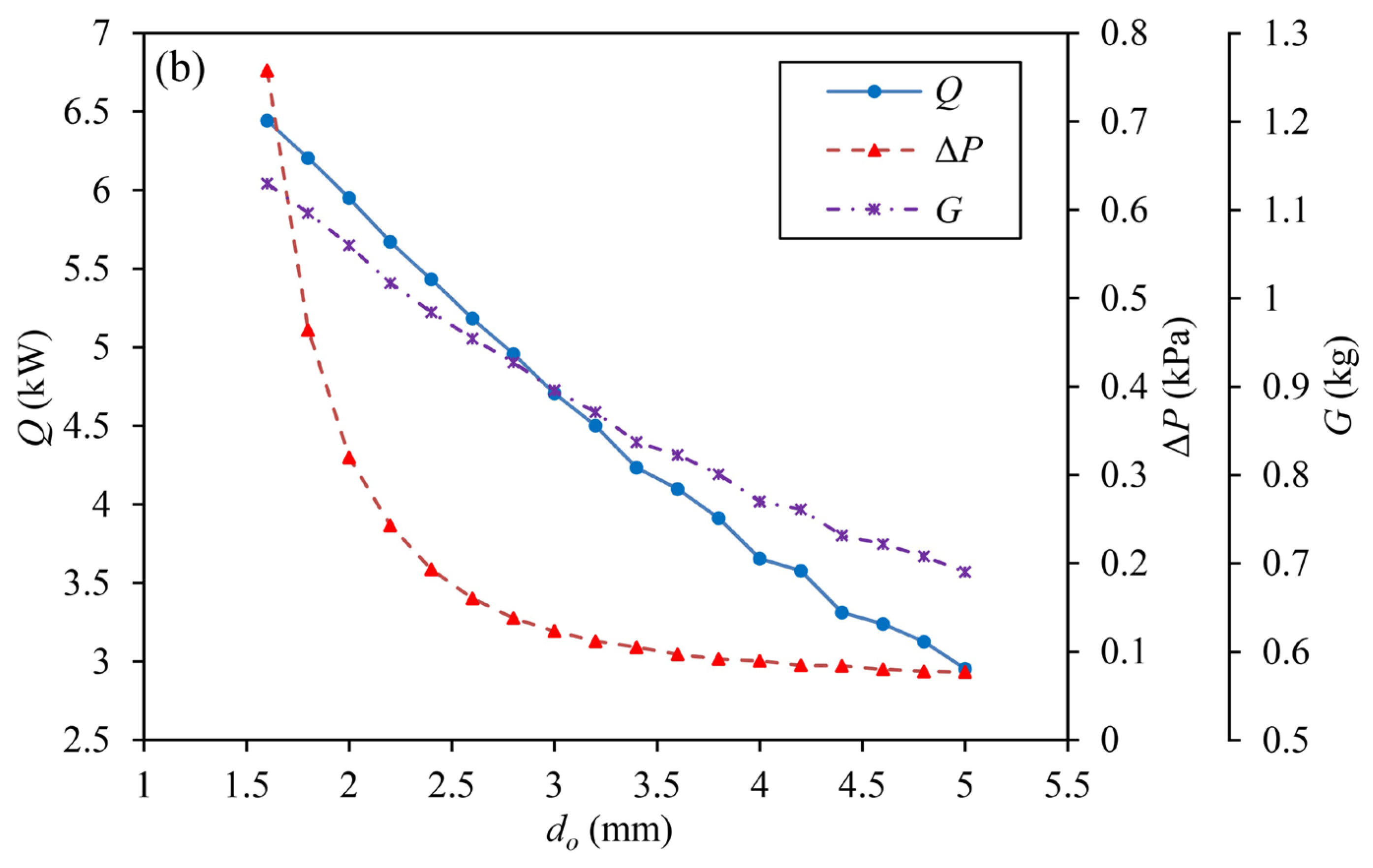
3.1.1. Influences of d_o

d_o varied from 1.6 mm to 5 mm while other structural parameters remained unchanged. The influences of d_o are presented in Figure 4.

As depicted in Figure 4a, while d_o increases from 1.6 mm to 5 mm, Q/ΔP increases from 8.50 W/Pa first, reaching its highest point of 42.66 W/Pa when d_o is 3.8 mm, and then generally reduces gradually to 38.37 W/Pa with slight oscillations, and Q/G decreases by 5.70–4.28 W/g. As d_o increases, heat dissipation tubes number decreases, and thus both heat transfer area and heat dissipation tubes weight decrease, which can result in heat transfer attenuation and weight reduction. In addition, the increase of d_o can cause the growth of tube-side flow area, thus the flow rate of the fluid inside heat dissipation tubes decreases, which can attenuate heat transfer and reduce tube-side on-way resistance. Thus, Q, ΔP, and G are all decreased with the increase of d_o, as illustrated in Figure 4b. Meanwhile, the reduction effect on tube-side on-way resistance of d_o increasing is gradually weakening. So, the reduce rate of ΔP is fast at the beginning and then gradually slow. Thus, Q/ΔP increases first and then decreases slowly after the effects of Q and ΔP reduce are almost equivalent. The slight oscillations of the Q/ΔP decreasing process are caused by the heat dissipation tubes number changing. As the change of heat dissipation tubes number is not continuous, the Q/ΔP line could be shaking, especially the variation effects of Q and ΔP are not much different. Thus, Q/ΔP increases first and then decreases slowly with slight oscillations, as shown in Figure 4a. Moreover, even though Q and G both decrease with the growth of d_o, Q always decreases faster than G. Hence, Q/G decreases continuously as shown in Figure 4a.

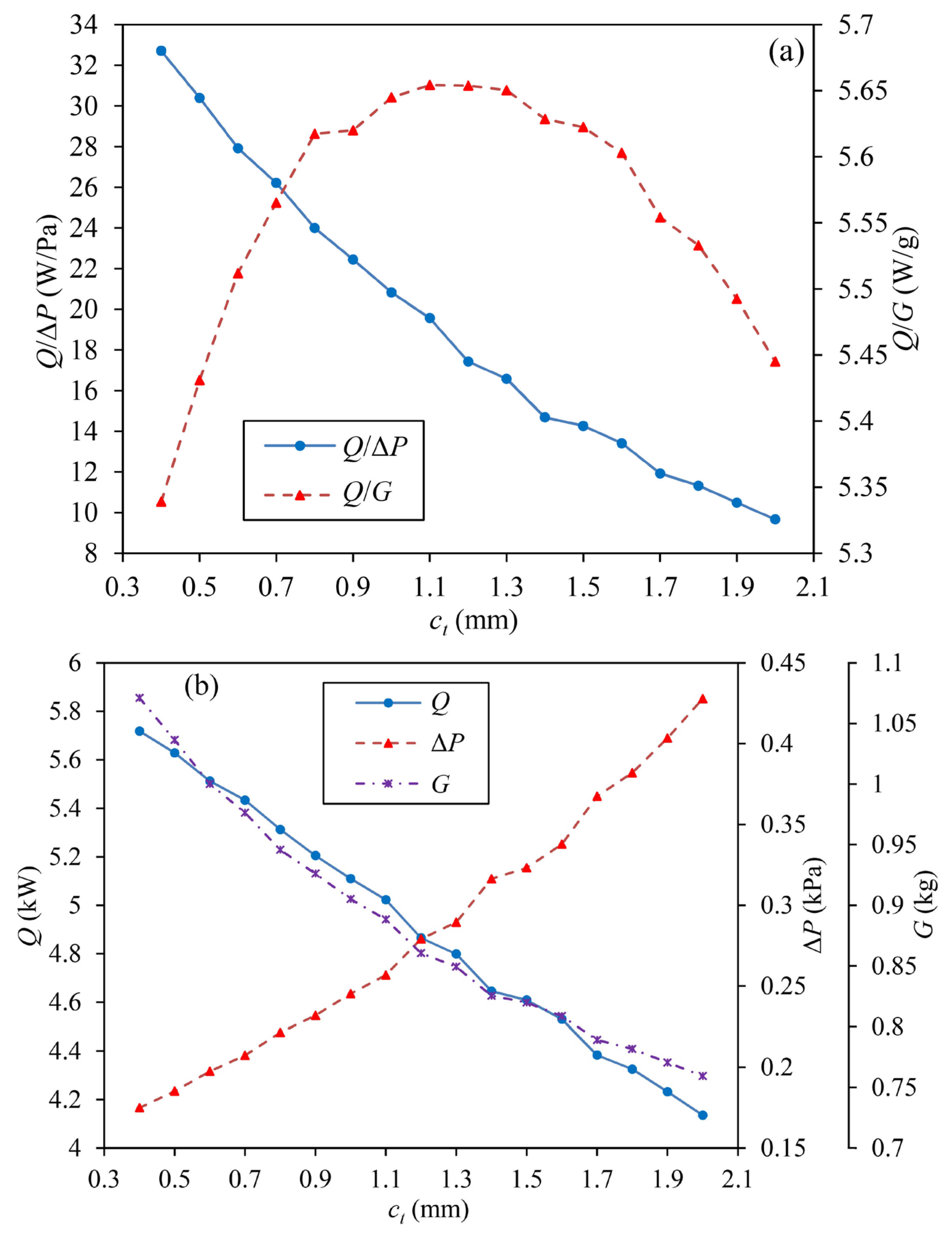
3.1.2. Influences of c_t

c_t varied from 0.4 mm to 2 mm while other structural parameters remained unchanged. The influences of c_t are presented in Figure 5.

As depicted in Figure 5a, while c_t increases from 0.4 mm to 2 mm, Q/ΔP decreases by 32.71–9.67 W/Pa, and Q/G increases from 5.34 W/g first, reaching its highest point of 5.65 W/g when c_t is 1.1 mm, and then reduces continuously to 5.45 W/g. Heat dissipation tubes number reduces with the increase of c_t, which can result in the reduction of heat transfer area and heat dissipation tubes weight and the growth of flow rate of the fluid inside heat dissipation tubes. Thus, both Q and G decrease, and ΔP increases, simultaneously, as illustrated in Figure 5b. As Q decreases and ΔP increases with the growth of c_t, Q/ΔP decreases steadily, as depicted in Figure 5a. In addition, even though both Q and G decrease, the decrease rate of Q is lower than G at the beginning, and then the decrease rate of Q is higher than G after c_t grows to one point. Thus, Q/G increases first and then decreases after peaking at one point, as shown in Figure 5a.

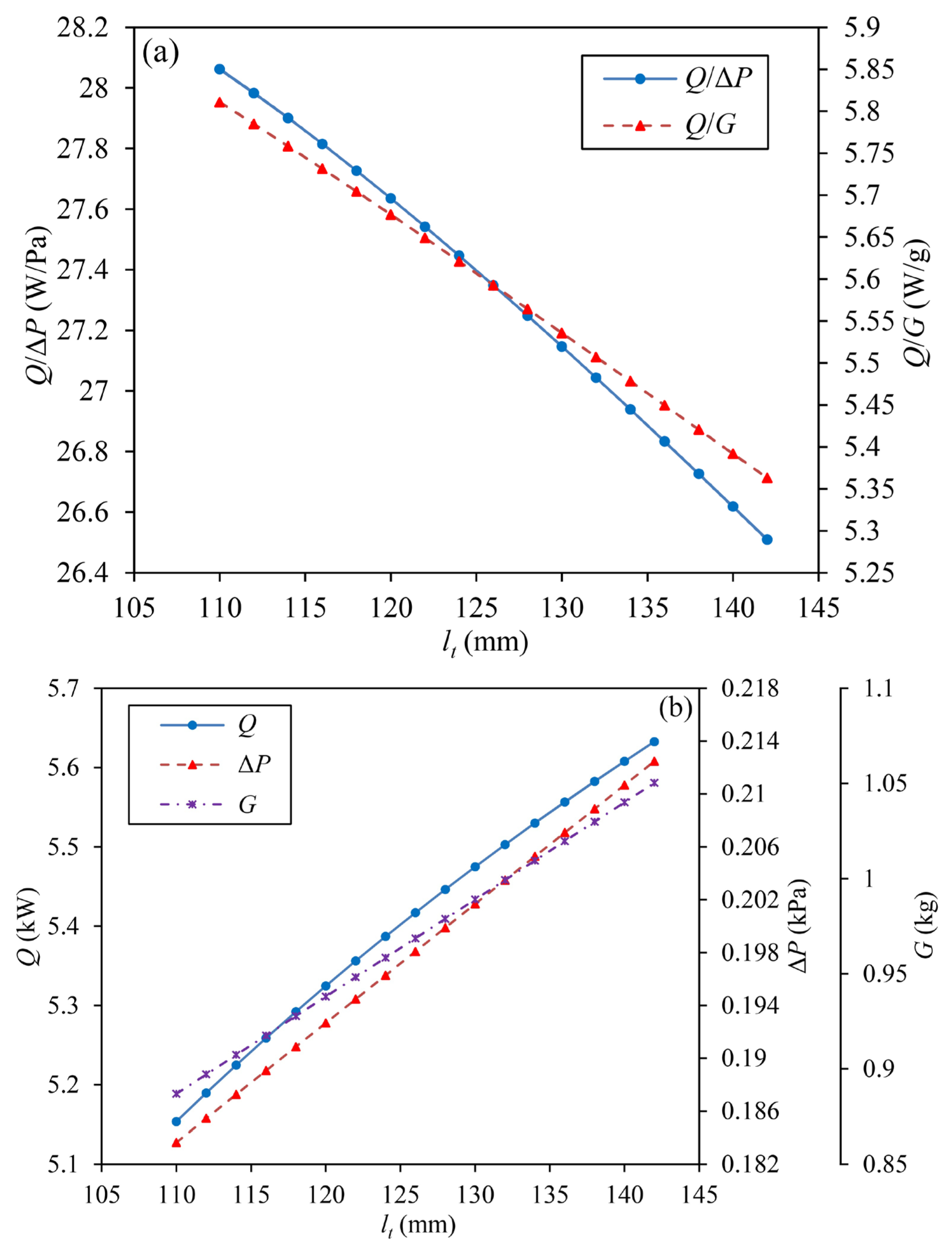
3.1.3. Influences of l_t

l_t varied from 110 mm to 142 mm while other structural parameters remained unchanged. The influences of l_t are presented in Figure 6.

As depicted in Figure 6a, while l_t increases from 110 mm to 142 mm, Q/ΔP and Q/G decrease by 28.06–26.51 W/Pa and 5.81–5.36 W/g, respectively. Heat transfer area, tube-side on-way resistance, and heat dissipation tubes weight are all increased with the growth of l_t, which results in the growth of Q, ΔP, and G, as illustrated in Figure 6b. Meanwhile, the growth rate of Q is lower than ΔP and G, which cause the continuously declining Q/ΔP and Q/G, as depicted in Figure 6a.

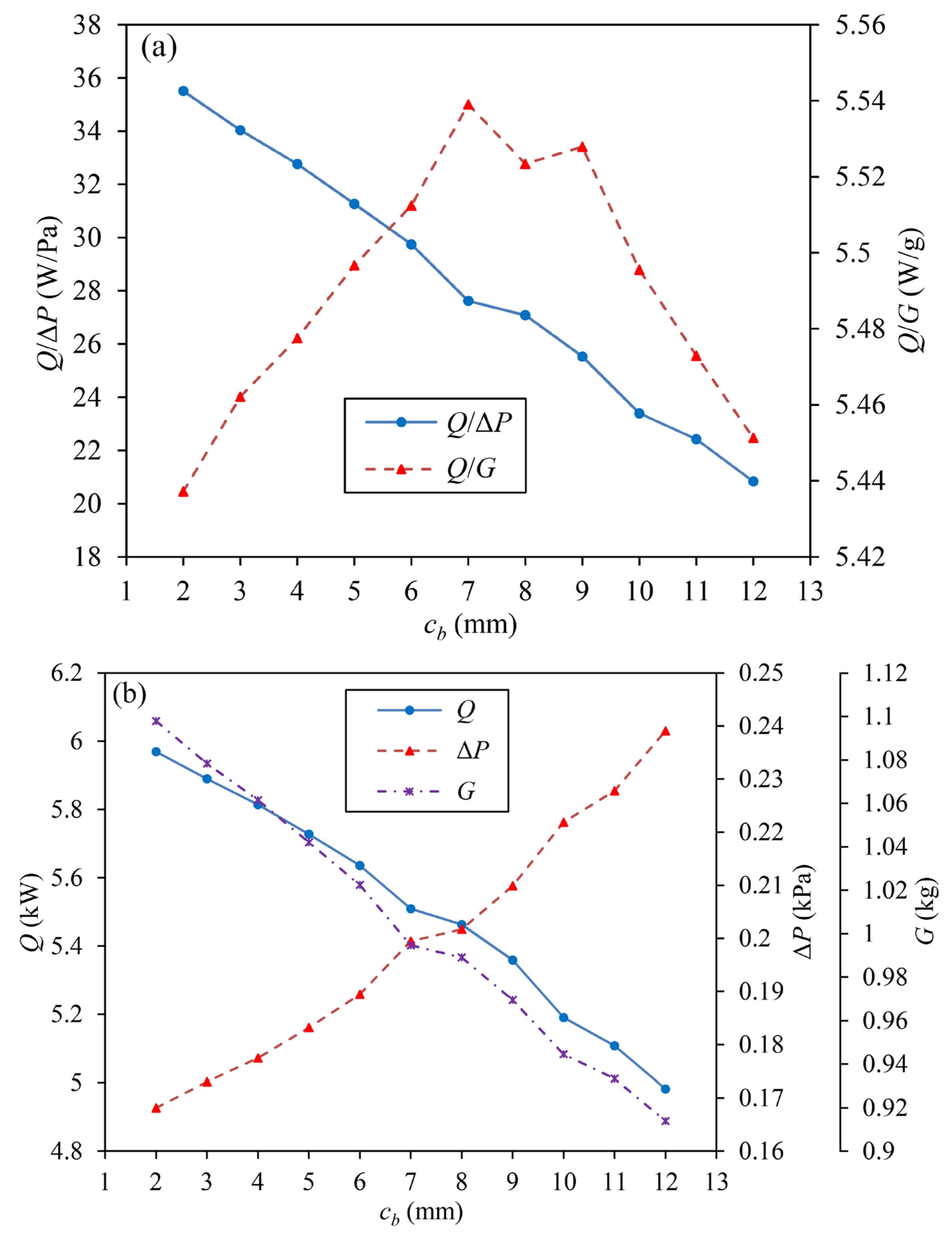
3.1.4. Influences of c_b

c_b varied from 2 mm to 12 mm while other structural parameters remained unchanged. The influences of c_b are presented in Figure 7.

As described in Figure 7a, while c_b increases from 2 mm to 12 mm, Q/ΔP decreases by 35.51–20.84 W/Pa, and Q/G increases from 5.44 W/g first, reaching its highest point of 5.54 W/g when c_b is 7 mm, then experiencing a small oscillation on the point that c_b is 8 mm, and then reduces to 5.45 W/g gradually. As c_b grows, heat dissipation tubes number declines, which can result in the reduction of heat transfer area and heat dissipation tubes weight and the increase of flow rate of the fluid inside heat dissipation tubes. Thus, both Q and G decline, and ΔP grows, simultaneously, as illustrated in Figure 7b. As Q decreases and ΔP increases, Q/ΔP decreases continuously with the growth of c_b, as depicted in Figure 7a. In addition, even though both Q and G decline, the decline rate of Q is lower than G at the beginning, and then the decline rate of Q is higher than G after c_b grows to one point. Thus, Q/G should increase first and then decrease. Meanwhile, the change of heat dissipation tubes number is not continuous, which results in Q/G line oscillation, especially when decline rates of Q and G are close, the oscillation phenomenon could become more severe. Hence, an oscillation occurs during the process of Q/G line reaching peak and gradually declining thereafter, as shown in Figure 7a.

3.2. Sensitivity Analysis

3.2.1. Sensitivity Analysis Using Sobol’ Method

The Sobol’ method [35,36] is one kind of widely employed global sensitivity analysis method based on variance, which can give out first-order sensitivity index that reflects a single input’s contribution to output and total sensitivity index that reflects the contribution of not only current input but also the interaction between current input and others to output. In this research, the Sobol’ method was adopted to analyze the influence contributions of d_o, c_t, l_t, and c_b on Q/ΔP and Q/G, as depicted by the following procedures:

(1)

Set input parameters as d_o, c_t, l_t, and c_b and output parameters as Q/ΔP and Q/G.

(2)

Set feasible region for input parameters and sampling size for Monte Carlo discretization.

(3)

Generate Sobol’ sequence and obtain sampling points using it.

(4)

Compute Q/ΔP and Q/G for sampling points based on STHX-SB design indicators calculation model.

(5)

Calculate first order sensitivity indices and total sensitivity indices of Q/ΔP and Q/G for d_o, c_t, l_t, and c_b utilizing Equations (30)~(35) [35,36,37].

$$S_i=\frac{D_i}{D_{tot}},\begin{array}{l}\hfill \end{array}for\begin{array}{l}\hfill \end{array}1\le i\le s,$$

(30)

$$S_{i\_tot}=\frac{D_{i\_tot}}{D_{tot}},\begin{array}{l}\hfill \end{array}for\begin{array}{l}\hfill \end{array}1\le i\le s,$$

(31)

$$D_{tot}={\displaystyle \int f^2(x)dx}-f_0^2\approx \frac{1}{N}{\displaystyle \sum _{k=1}^N{f}^2(x_k)}-f_0^2,$$

(32)

$$D_i=D_{tot}-\frac{1}{2}{\displaystyle \int {[f(x)-f(x_i,x{\prime }_{-i})]}^{2}dxdx{\prime }_{-i}}\approx D_{tot}-\frac{1}{2N}{\displaystyle \sum _{k=1}^N{[f(x_k)-f(x_{ik},x{\prime }_{-ik})]}^2},$$

(33)

$$D_{i\_tot}=\frac{1}{2}{\displaystyle \int {[f(x)-f(x{\prime }_i,x_{-i})]}^{2}dxdx{\prime }_{-i}}\approx \frac{1}{2N}{\displaystyle \sum _{k=1}^N{[f(x_k)-f(x{\prime }_{ik},x_{-ik})]}^2},$$

(34)

$$f_0={\displaystyle \int f(x)dx}\approx \frac{1}{N}{\displaystyle \sum _{k=1}^{N}f(x_k)},$$

(35)

3.2.2. Sensitivity Analysis Results

In this research, the feasible region for input parameters was set as shown by Equation (36). N was set as 100,000. The obtained sensitivity indices of Q/ΔP and Q/G for d_o, c_t, l_t, and c_b are shown in Figure 8.

$$\left\{\begin{array}{l}1.6\mathrm{mm}\le d_o\le 5\mathrm{mm}\hfill \\ 0.4\mathrm{mm}\le c_t\le 2\mathrm{mm}\hfill \\ 110\mathrm{mm}\le l_t\le 142\mathrm{mm}\hfill \\ 2\mathrm{mm}\le c_b\le 12\mathrm{mm}\hfill \end{array}\right.,$$

(36)

It could be found from Figure 8 that for these two kinds of indices, the indices of Q/ΔP for d_o are both the highest followed by c_t, c_b, l_t, and the indices of Q/G for d_o are both the highest followed by c_b, c_t, l_t. Thus, it can be considered that whether the interaction between factors is considered or not, both Q/ΔP and Q/G are the most sensitive to changes in d_o and the least sensitive to changes in l_t.

4. Configuration Optimization

4.1. Configuration Optimization Method

4.1.1. Problem Presentation

According to previous parametric study, it is obvious that the changing of Q/ΔP and Q/G is in connection with the variation of d_o, c_t, l_t, and c_b. Hence, in order to improve STHX-SB comprehensive performance, d_o, c_t, l_t, and c_b, as shown in Figure 1, were optimized to maximize Q/ΔP and Q/G, simultaneously. This problem is formulated by Equation (37).

$$\left\{\begin{array}{ll}Max\hfill & Q/\Delta P,Q/G\hfill \\ S.t.\hfill & 1.6\mathrm{mm}\le d_o\le 5\mathrm{mm}\hfill \\ \hfill & 0.4\mathrm{mm}\le c_t\le 2\mathrm{mm}\hfill \\ \hfill & 110\mathrm{mm}\le l_t\le 142\mathrm{mm}\hfill \\ \hfill & 2\mathrm{mm}\le c_b\le 12\mathrm{mm}\hfill \end{array}\right.,$$

(37)

4.1.2. Combination Optimization of NSGAII and MOPSO Embedded Grouping Cooperative Coevolution

From previous parametric studies, it is not difficult to be found that the influences of d_o, c_t, l_t, and c_b on Q/ΔP and Q/G are nonlinear and conflicted in most cases. Simultaneous changings of d_o, c_t, l_t, and c_b can result in complicated simultaneous variations of Q/ΔP and Q/G, which can make satisfactory optimal solutions hard to pick out utilizing simple parametric study only. When encountering this kind of situation, adopting multi-objective optimization theory can be a feasible solution.

To avoid the problem of falling into local optima due to algorithm convergence being too fast and to improve the reliability of solving multidimensional large-scale complex optimization problems, a cooperative coevolution method that embeds grouping optimization strategy into multi-objective optimization theory was proposed, which groups configuration parameters according to their contributions to performance indicators and then realizes initial optimization of grouping and secondary optimization after merging various groups based on a strategy of multi-objective optimization algorithm driving design indicators prediction model. NSGAII [38] and MOPSO [39] are two classic and significant optimization methods. However, NSGAII has the limitation of lower convergence and MOPSO has the limitation of easily trapping into local optima. Thus, in this research, NSGAII was adopted in the initial optimization of grouping and MOPSO was adopted in the secondary optimization after merging various groups in the process of cooperative coevolution, which can realize complementary deficiencies between NSGAII and MOPSO. Ultimately, one combination optimization method of NSGAII and MOPSO embedded grouping cooperative coevolution (NSGAII-MOPSO-GCC) can be proposed. The procedures of STHX-SB configuration optimization based on NSGAII-MOPSO-GCC are presented as follows:

(1)

Define design parameters, feasible region, and optimization objectives.

(2)

Retrieve Sobol’ sensitivity analysis results in parametric study.

(3)

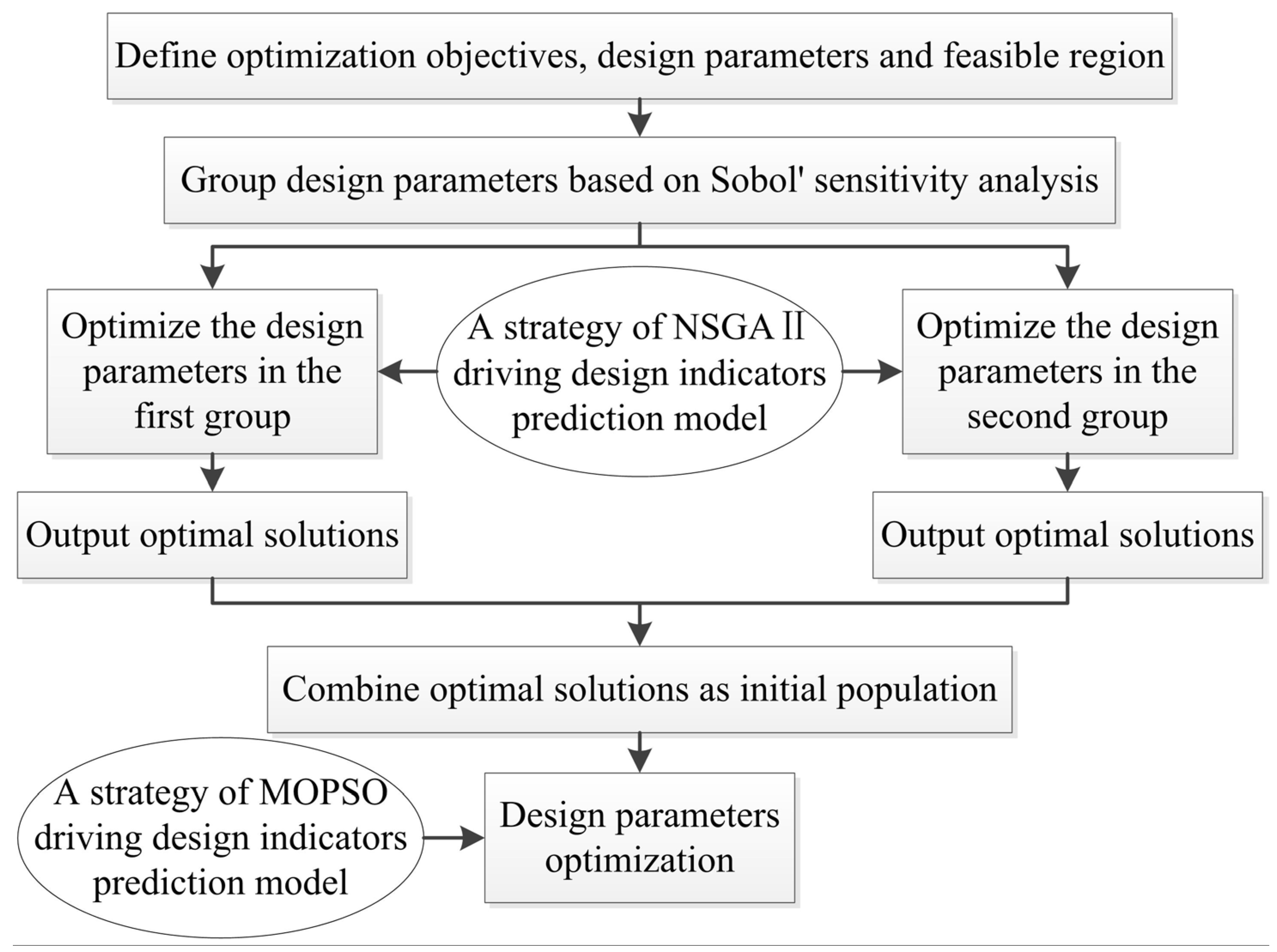
Group design parameters according to the contributions of design parameters to objective functions. In this research, this procedure is conducted as follows:

(a)

Select 50% of the design parameters that the first objective function is more sensitive to.

(b)

Select 50% of the design parameters that the second objective function is more sensitive to.

(c)

Combine the design parameters selected in Step (a) and Step (b) as the first group.

(d)

Select 50% of the design parameters that the first objective function is less sensitive to.

(e)

Select 50% of the design parameters that the second objective function is less sensitive to.

(f)

Combine the design parameters selected in Step (d) and Step (e) as the second group.

(4)

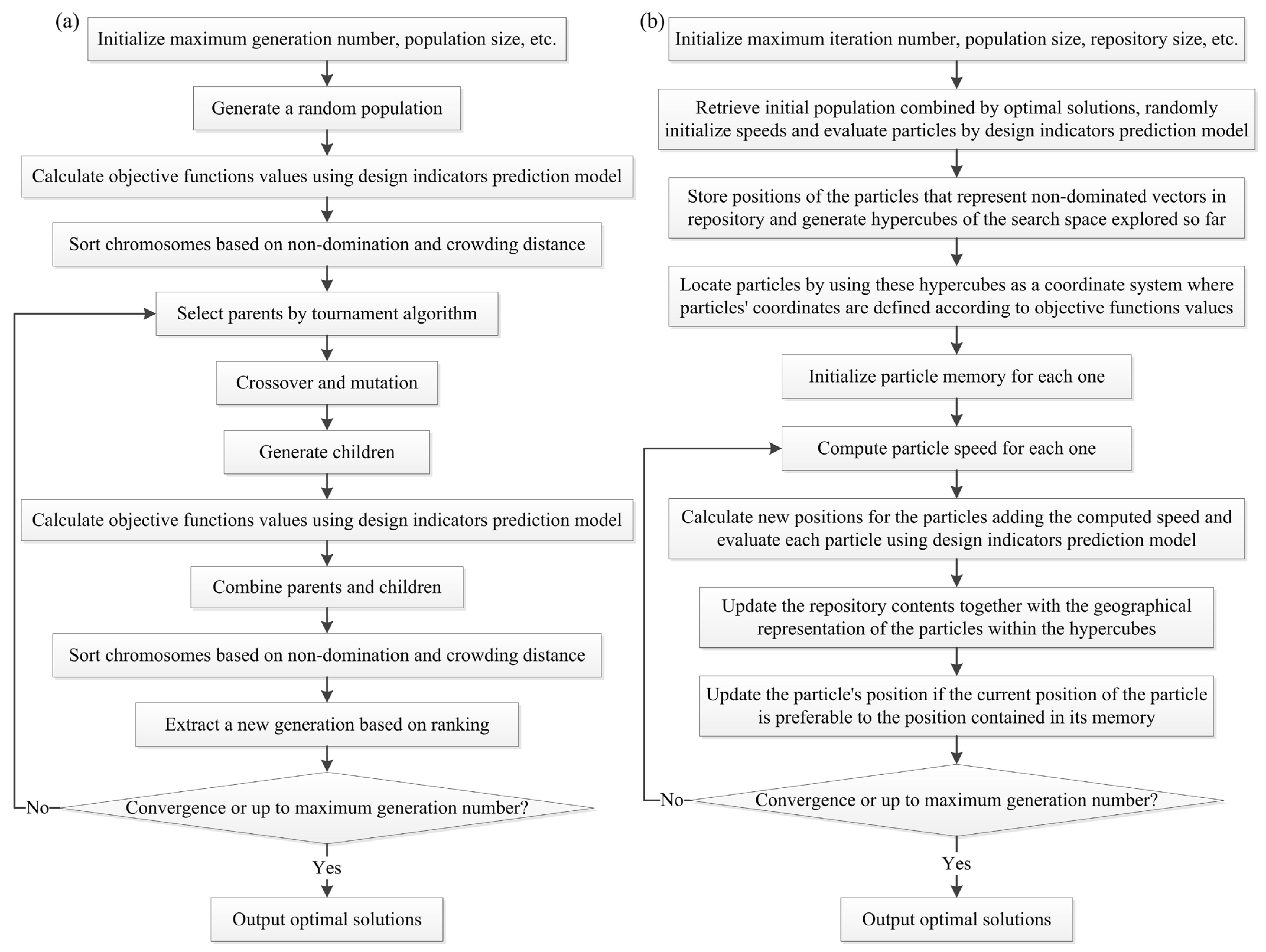
Optimize the design parameters in the first group and the second group, respectively, based on a strategy of NSGAII driving design indicators prediction model. NSGAII optimization flow is depicted by Figure 9a.

(5)

Combine the optimal solutions of the two groups as initial population and optimize the design parameters shown by Equation (37) based on a strategy of MOPSO driving design indicators prediction model. MOPSO optimization flow is depicted by Figure 9b.

Figure 9. Optimization flows of NSGAII and MOPSO: (a) NSGAII; (b) MOPSO.

Figure 9. Optimization flows of NSGAII and MOPSO: (a) NSGAII; (b) MOPSO.

The illustration of STHX-SB configuration optimization flow based on NSGAII-MOPSO-GCC is depicted in Figure 10.

4.2. Optimization Results

According to the previous Sobol’ analysis in this research, Q/ΔP is the most sensitive to d_o and then followed by c_t, c_b, l_t, and Q/G is the most sensitive to d_o and then followed by c_b, c_t, l_t. Thus, d_o, c_t, and c_b were arranged in the first group of the design parameters that the objective functions are more sensitive to, and c_t, l_t, and c_b were arranged in the second group of the design parameters that the objective functions are less sensitive to. Population size and maximum generation number of NSGAII in NSGAII-MOPSO-GCC were 100 and 50, respectively. Repository size, population size, and maximum iteration number of MOPSO in NSGAII-MOPSO-GCC were 100, 200, and 50, respectively. The obtained optimal solutions by NSGAII-MOPSO-GCC are shown by Figure 10, and it is not hard to be found that some Pareto optimal solutions obtained by NSGAII-MOPSO-GCC can achieve higher Q/ΔP and higher Q/G simultaneously compared with the original configuration. Three solutions were chosen from them, as shown in Figure 11 and

Table 6. Optimal solutions comparison.

Parameters	do (mm)	ct (mm)	lt (mm)	cb (mm)	Q/ΔP (W/Pa)	Q/G (W/g)
Original	2.36	0.64	130	7.5	27.14	5.54
Solution A	2.26	0.93	110	2.1	27.45	6.03
Solution B	2.70	0.74	110	2.0	42.74	5.81
Solution C	3.39	0.40	115	2.0	58.18	5.55

.

As illustrated in Table 6, Q/ΔP of solutions A, B, and C increases separately by 1.14%, 57.48%, and 114.37%, and simultaneously, Q/G of solutions A, B, and C increases separately by 8.84%, 4.87%, and 0.18%, compared with the original structure. For the selected solutions, the average improvement percentages of Q/ΔP and Q/G are 57.66% and 4.63%, respectively. Thus, through NSGAII-MOPSO-GCC, maximizing Q/ΔP and Q/G simultaneously can be realized reliably.

In addition, optimization comparison among NSGAII-MOPSO-GCC and two classic optimization methods including NSGAII and MOPSO was also conducted. In order to ensure comparability, population size and maximum generation number of NSGAII were both set as 100, and repository size, population size, and maximum iteration number of MOPSO were separately set as 100, 200, and 100. The comparison results are depicted in Figure 10, and it can be clearly seen that Q/ΔP and Q/G values of almost all of the optimal points obtained by NSGAII-MOPSO-GCC and MOPSO are higher than the values obtained by NSGAII, which indicates that NSGAII has the lowest convergence rate among them. Moreover, even though many of the optimal points obtained by MOPSO almost overlap with the optimal points obtained by NSGAII-MOPSO-GCC, there still exist some optimal points searched by NSGAII-MOPSO-GCC that are not found by MOPSO, especially the optimal solutions in the Q/ΔP range of higher than 57.92 W/Pa, which indicates that the searching capability of MOPSO is lower than NSGAII-MOPSO-GCC as MOPSO has the limitation of easily trapping into local optima. Thus, it can be concluded that among these three optimization methods, NSGAII-MOPSO-GCC performs the best, followed by MOPSO, and then NSGAII. Hence, based on the analysis above, it can be considered that the proposed method of STHX-SB configuration optimization based on NSGAII-MOPSO-GCC is valid and feasible, which can supply beneficial and valuable guidance in engineer applications of heat exchanger.

5. Conclusions

In this research, one design indicators prediction model for STHX-SB based on the Bell–Delaware method was constructed to calculate Q, ΔP, and G, and the model reliability was validated. Based on a design indicators prediction model, a parametric study was conducted to research the influences of d_o, c_t, l_t, and c_b on Q/ΔP and Q/G and analyze the sensitivity indices of d_o, c_t, l_t, and c_b for Q/ΔP and Q/G utilizing the Sobol’ method. Based on the design indicators prediction model and Sobol’ sensitivity analysis theory, one combination optimization method of NSGAII-MOPSO-GCC was proposed for STHX-SB to optimize d_o, c_t, l_t, and c_b to maximize Q/ΔP and Q/G simultaneously. Comparison between three selected optimal solutions and the original configuration was conducted. In addition, optimization effects among NSGAII-MOPSO-GCC and two classic optimization algorithms including NSGAII and MOPSO were compared. Below are the main conclusions:

(1)

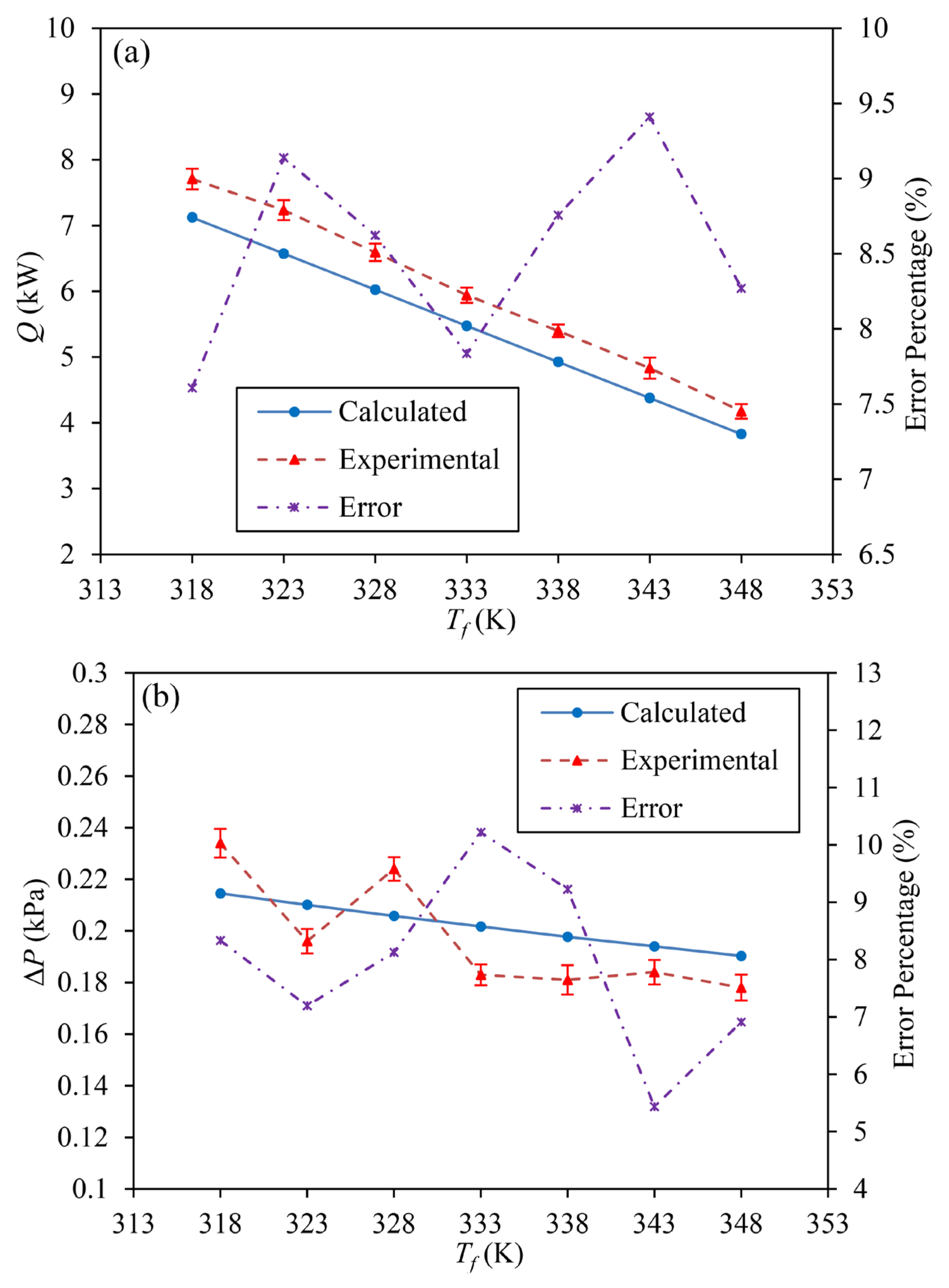
Compared with experimental data, the error percentages of Q are 7.61–9.41% with the average value of 8.52%, and the error percentages of ΔP are 5.43–10.22% with the average value of 7.92%. The values of G predicted by the proposed model and weighed by Solidworks commercial software are the same. So, the proposed design indicators prediction model is validated to be reliable and valid.

(2)

Through parametric influences analysis, it can be found that Q/ΔP grows first and then declines slightly with slight oscillations with the increase of d_o, and it reduces with the increase of anyone of c_t, l_t, and c_b. Q/G decreases with the increase of anyone of d_o and l_t, and it rises first and then reduces with the increase of c_t. As c_b grows, Q/G increases first, experiencing a small oscillation after peaking at a point, and then reduces.

(3)

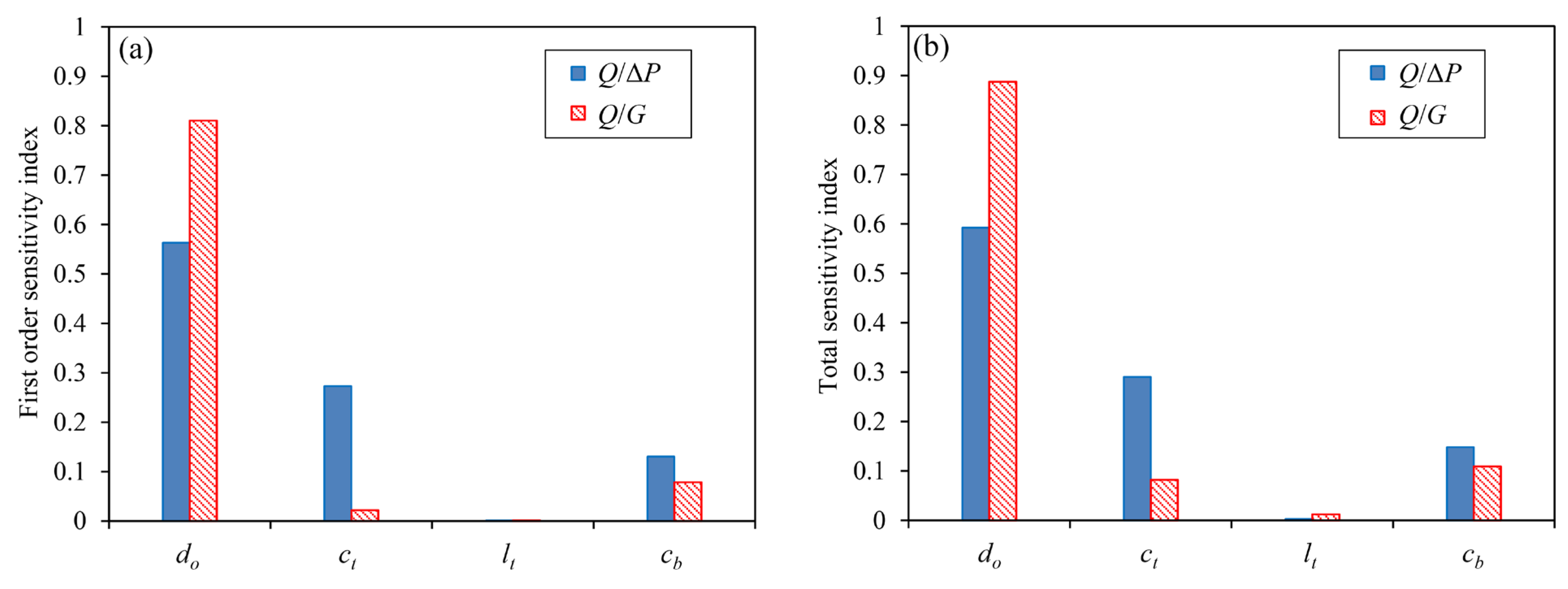
Through Sobol’ sensitivity analysis, it can be found that whether the interaction between factors is considered or not, Q/ΔP is the most sensitive to d_o and then followed by c_t, c_b, l_t, and Q/G is the most sensitive to d_o and then followed by c_b, c_t, l_t.

(4)

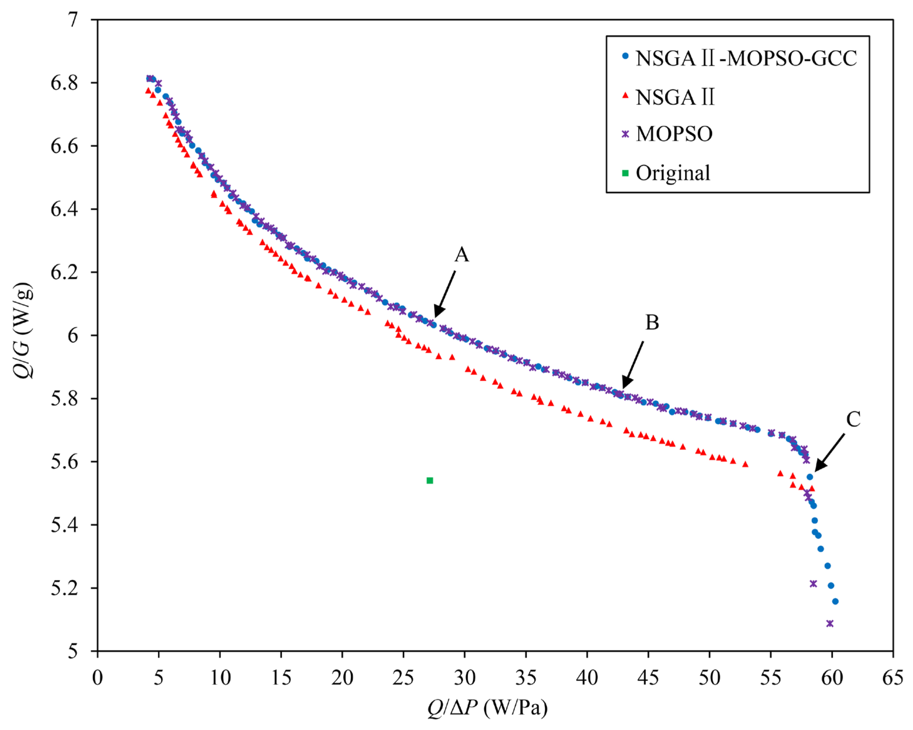
For the selected solutions, the average improvement percentages of Q/ΔP and Q/G separately are 57.66% and 4.63%, compared with the original structure, and through the comparison among the three optimization algorithms, it can be found that NSGAII-MOPSO-GCC performs the best, followed by MOPSO, and then NSGAII, which illustrates that the proposed method of STHX-SB configuration optimization based on NSGAII-MOPSO-GCC is valid and feasible, and can supply beneficial and valuable guidance for heat exchanger design and improvement.

References

- Močnik, U.; Muhič, S. Experimental and numerical analysis of heat transfer in a dimple pattern heat exchanger channel. Appl. Therm. Eng. 2023, 230, 120865. [Google Scholar] [CrossRef]
- Wang, J.; Sun, L.; Li, H.; Ding, R.; Chen, N. Prediction model of fouling thickness of heat exchanger based on TA-LSTM structure. Processes 2023, 11, 2594. [Google Scholar] [CrossRef]
- Lima, C.C.; Ochoa, A.A.; da Costa, J.A.; de Menezes, F.D.; Alves, J.V.; Ferreira, J.M.; Azevedo, C.C.; Michima, P.S.; Leite, G.N. Experimental and computational fluid dynamic—CFD analysis simulation of heat transfer using graphene nanoplatelets GNP/water in the double tube heat exchanger. Processes 2023, 11, 2735. [Google Scholar] [CrossRef]
- Mann, G.W.; Eckels, S. Multi-objective heat transfer optimization of 2D helical micro-fins using NSGA-II. Int. J. Heat Mass Transf. 2019, 132, 1250–1261. [Google Scholar] [CrossRef]
- Dehaj, M.S.; Hajabdollahi, H. Fin and tube heat exchanger: Constructal thermo-economic optimization. Int. J. Heat Mass Transf. 2021, 173, 121257. [Google Scholar] [CrossRef]
- Esfe, M.H.; Mahian, O.; Hajmohammad, M.H.; Wongwises, S. Design of a heat exchanger working with organic nanofluids using multi-objective particle swarm optimization algorithm and response surface method. Int. J. Heat Mass Transf. 2018, 119, 922–930. [Google Scholar] [CrossRef]
- Dagdevir, T. Multi-objective optimization of geometrical parameters of dimples on a dimpled heat exchanger tube by Taguchi based Grey relation analysis and response surface method. Int. J. Therm. Sci. 2022, 173, 107365. [Google Scholar] [CrossRef]
- de Vasconcelos Segundo, E.H.; Amoroso, A.L.; Mariani, V.C.; dos Santos Coelho, L. Economic optimization design for shell-and-tube heat exchangers by a Tsallis differential evolution. Appl. Therm. Eng. 2017, 111, 143–151. [Google Scholar] [CrossRef]
- de Vasconcelos Segundo, E.H.; Mariani, V.C.; dos Santos Coelho, L. Design of heat exchangers using falcon optimization algorithm. Appl. Therm. Eng. 2019, 156, 119–144. [Google Scholar] [CrossRef]
- Li, B.; Li, Z.; Yang, P.; Xu, J.; Wang, H. Modeling and optimization of the thermal-hydraulic performance of direct contact heat exchanger using quasi-opposite Jaya algorithm. Int. J. Therm. Sci. 2022, 173, 107421. [Google Scholar] [CrossRef]
- Liu, A.; Wang, G.; Wang, D.; Peng, X.; Yuan, H. Study on the thermal and hydraulic performance of fin-and-tube heat exchanger based on topology optimization. Appl. Therm. Eng. 2021, 197, 117380. [Google Scholar] [CrossRef]
- Singh, S.; Akhil, B.V.; Chowdhury, S.; Lahiri, S.K. A detailed insight into the optimization of plate and frame heat exchanger design by comparing old and new generation metaheuristics algorithms. J. Indian Chem. Soc. 2022, 99, 100313. [Google Scholar] [CrossRef]
- Zhang, Y.; Peng, J.; Yang, R.; Yuan, L.; Li, S. Weight and performance optimization of rectangular staggered fins heat exchangers for miniaturized hydraulic power units using genetic algorithm. Case Stud. Therm. Eng. 2021, 28, 101605. [Google Scholar] [CrossRef]
- Iyer, V.H.; Mahesh, S.; Malpani, R.; Sapre, M.; Kulkarni, A.J. Adaptive range genetic algorithm: A hybrid optimization approach and its application in the design and economic optimization of shell-and-tube heat exchanger. Eng. Appl. Artif. Intell. 2019, 85, 444–461. [Google Scholar] [CrossRef]
- Wen, J.; Gu, X.; Wang, M.; Liu, Y.; Wang, S. Multi-parameter optimization of shell-and-tube heat exchanger with helical baffles based on entransy theory. Appl. Therm. Eng. 2018, 130, 804–813. [Google Scholar] [CrossRef]
- Lim, H.; Han, U.; Lee, H. Design optimization of bare tube heat exchanger for the application to mobile air conditioning systems. Appl. Therm. Eng. 2020, 165, 114609. [Google Scholar] [CrossRef]
- Wen, J.; Gu, X.; Wang, M.; Wang, S.; Tu, J. Numerical investigation on the multi-objective optimization of a shell-and-tube heat exchanger with helical baffles. Int. Commun. Heat Mass Transf. 2017, 89, 91–97. [Google Scholar] [CrossRef]
- Wang, S.; Xiao, J.; Wang, J.; Jian, G.; Wen, J.; Zhang, Z. Configuration optimization of shell-and-tube heat exchangers with helical baffles using multi-objective genetic algorithm based on fluid-structure interaction. Int. Commun. Heat Mass Transf. 2017, 85, 62–69. [Google Scholar] [CrossRef]
- Wang, S.; Xiao, J.; Wang, J.; Jian, G.; Wen, J.; Zhang, Z. Application of response surface method and multi-objective genetic algorithm to configuration optimization of Shell-and-tube heat exchanger with fold helical baffles. Appl. Therm. Eng. 2018, 129, 512–520. [Google Scholar] [CrossRef]
- Wang, S.; Jian, G.; Xiao, J.; Wen, J.; Zhang, Z.; Tu, J. Fluid-thermal-structural analysis and structural optimization of spiral-wound heat exchanger. Int. Commun. Heat Mass Transf. 2018, 95, 42–52. [Google Scholar] [CrossRef]
- Wang, X.; Zheng, N.; Liu, Z.; Liu, W. Numerical analysis and optimization study on shell-side performances of a shell and tube heat exchanger with staggered baffles. Int. J. Heat Mass Transf. 2018, 124, 247–259. [Google Scholar] [CrossRef]
- Ocłoń, P.; Łopata, S.; Stelmach, T.; Li, M.; Zhang, J.F.; Mzad, H.; Tao, W.Q. Design optimization of a high-temperature fin-and-tube heat exchanger manifold-a case study. Energy 2021, 215, 119059. [Google Scholar] [CrossRef]
- Keramati, H.; Hamdullahpur, F.; Barzegari, M. Deep reinforcement learning for heat exchanger shape optimization. Int. J. Heat Mass Transf. 2022, 194, 123112. [Google Scholar] [CrossRef]
- Saijal, K.K.; Danish, T. Design optimization of a shell and tube heat exchanger with staggered baffles using neural network and genetic algorithm. Proc. Inst. Mech. Eng. Part C: J. Mech. Eng. Sci. 2021, 235, 5931–5946. [Google Scholar] [CrossRef]
- Tang, C.; Liu, H.; Tang, X.; Wei, L.; Shao, X.; Xie, G. Thermal Performance and Parametrical Analysis of Topologically-optimized Cross-flow Heat Sinks Integrated with Impact Jet. Appl. Therm. Eng. 2023, 235, 121310. [Google Scholar] [CrossRef]
- Lin, J.; Chang, C.; Yang, J. Transmission and Lubrication System: Aeroengine Design Manual; Aviation Industry Press: Beijing, China, 2002; Volume 12. [Google Scholar]
- Liu, J. China Jet Fuel; China Petrochemical Press: Beijing, China, 1991. [Google Scholar]
- Bell, K.J. Final Report of the Cooperative Research Program on Shell-and-Tube Heat Exchangers; University of Delaware, Engineering Experimental Station: Newark, DE, USA, 1963. [Google Scholar]
- Qian, S. Heat Exchanger Design Manual; Chemistry Industry Publisher: Beijing, China, 2002. [Google Scholar]
- Kuppan, T. Heat Exchanger Design Handbook; CRC Press: New York, NY, USA, 2013. [Google Scholar]
- Shah, R.K.; Sekulic, D.P. Fundamentals of Heat Exchanger Design; John Wiley & Sons: New York, NY, USA, 2003. [Google Scholar]
- Shi, M.; Wang, Z. Principle and Design of Heat Exchangers, 4th ed.; Southeast University Press: Nanjing, China, 2009. [Google Scholar]
- Kays, W.M.; London, A.L. Compact Heat Exchangers; McGraw-Hill: New York, NY, USA, 1984. [Google Scholar]
- Dong, Q.; Zhang, Y. Petrochemical Equipment Design and Selection Manual: Heat Exchanger; Chemistry Industry Publisher: Beijing, China, 2008. [Google Scholar]
- Sobol’, I.M. Sensitivity analysis for non-linear mathematical models. Math. Model. Comput. Exp. 1993, 1, 407–414. [Google Scholar]
- Sobol’, I.M. Global sensitivity indices for nonlinear mathematical models and their Monte Carlo estimates. Math. Comput. Simul. 2001, 55, 271–280. [Google Scholar] [CrossRef]
- Zheng, Y.; Rundell, A. Comparative study of parameter sensitivity analyses of the TCR-activated Erk-MAPK signalling pathway. IEE Proc. Syst. Biol. 2006, 153, 201–211. [Google Scholar] [CrossRef]
- Srinivas, N.; Deb, K. Muiltiobjective optimization using nondominated sorting in genetic algorithms. Evol. Comput. 1994, 2, 221–248. [Google Scholar] [CrossRef]
- Coello, C.A.C.; Pulido, G.T.; Lechuga, M.S. Handling multiple objectives with particle swarm optimization. IEEE Trans. Evol. Comput. 2004, 8, 256–279. [Google Scholar] [CrossRef]