Dynamic Optimisation of Fed-Batch Bioreactors for mAbs: Sensitivity Analysis of Feed Nutrient Manipulation Profiles

Abstract

Successful cultivation of mammalian cells must consider careful formulation of culture media consisting of a variety of substrates and amino acids. A widely cited method for quantifying metabolic networks of mammalian cultures is dynamic flux balance modelling. Application of in-silico techniques allows researchers to circumvent time-consuming and costly in-vivo experimentation. Dynamic simulation and optimisation of reliable models allows for the visualization of opportunities to improve throughputs of target protein products, such as monoclonal antibodies (mAbs). This study presents a sensitivity analysis comparing dynamic optimisation results for industrial-scale fed-batch bioreactors, considering a variety of initial conditions. Optimized feeding trajectories are computed via Nonlinear Programming (NLP) model, employing the established IPOPT solver. Glucose, then glutamine, then asparagine, can lead to improved mAb yields and viable cell counts.

1. Introduction

Monoclonal antibodies (mAbs) are a class of biotherapeutics with great potential to treat a number of ailments, including (but not limited to) cancers and autoimmune diseases [1,2]. mAbs are genetically engineered proteins which are cultivated in laboratories using mammalian cell cultures, e.g., Chinese Hamster Ovary/CHO cells [3]. Mammalian cultures are necessary for successful mAb production due to complex post-translational changes (e.g., glycosylation) needed to ensure mAb efficacy, and only feasible to achieve with a complex mammalian genome structure [4]. The first mAb given market approval by the US FDA was muromonab-CD3 in 1986 [5]. As of 2018, there were 78 mAbs given market approval and the mAb market had reached a value of USD 115.2 billion [6] and rising. The strong increasing trend in the total mAb market value is illustrated in Figure 1 [7].

The modern approach to industrial-scale upstream manufacture of mAbs is the fed-batch (FB) operation of large bioreactor vessels (Figure 2). In these systems, the seeded culture is used to inoculate the substrate feed, whose feeding strategy is implemented as a series of pulse and step inputs: removal of bioreactor contents occurs intermittently at the/end of every campaign. The substrate selected depends on the elementary flux mode (key metabolic pathway) manipulated, but the most common substrates fed are those which are involved in product-relevant modes. Metabolic pathways of importance to general function (and consequently mAb production) include glycolysis, tricarboxylic acid cycle, amino acid cycle, pentose phosphate and nucleic acid synthesis [8]. In mammalian cell cultures, the substrates most commonly manipulated are glucose, glutamine and asparagine [9], due to their vital roles in many of the modes mentioned. Currently, there is a gap of knowledge of which substrates play the most important role towards cell function and culture growth. Furthermore, more insight could be provided to quantify the effects of changing initial substrate concentration on culture growth and mAb titer trajectories.

Dynamic optimisation techniques which elucidate fed-batch feeding strategies that improve total mAb throughput have been extensively employed in the literature [10,11,12,13,14,15,16,17,18]. Technoeconomic studies which analyse cost implications and possible benefits in detail abound [19,20,21], towards the transition to (currently costlier) continuous operation [22,23,24,25,26]. This study presents a series of dynamic optimisations for final mAb titer maximisation at the end of bioreactor operation, employing a published dynamic flux balance model considering elementary flux modes of a glutamine synthetase-CHO culture (GS-CHO) [27]. Glucose, glutamine and asparagine are the three substrates explored as manipulated feed input: initial conditions for each of these substrate feeds are varied, with one low and one high concentration condition. This variation in the type and initial concentration of the feed becomes the basis of a sensitivity analysis, which quantifies the consequence of six (6) feeding strategies on GS-CHO culture performance. The numerical trends established provide unique insight into which substrates are of most importance to mAb cultivation.

2. Materials and Methods

2.1. Dynamic Flux Balance Model

The dynamic model adapted from Yilmaz et al. [27] is in Appendix A (

Table A1. The dynamic flux balance model as per Yilmaz et al., (2020) [27].

${GLC}_{ex}+\left(\frac{14}{3}\right)NA{D}_m^{+}+4ADP\underset{}{\to }6C{O}_2+\left(\frac{17}{3}\right)NAD{H}_m+4ATP$	(R1)
${GLC}_{ex}+2ADP\underset{}{\to }{LAC}_{ex}+2ATP$	(R2)
${PYR}_{ex}+\left(\frac{14}{3}\right)NA{D}_m^{+}+ADP\underset{}{\to }3C{O}_2+\left(\frac{14}{3}\right)NAD{H}_m+ATP$	(R3)
${GLN}_{ex}\underset{}{\to }{GLU}_{ex}+N{H}_{4ex}$	(R4)
${GLN}_{ex}+\left(\frac{25}{3}\right)NA{D}_m^{+}+ADP\underset{}{\to }5C{O}_2+\left(\frac{25}{3}\right)NAD{H}_m+ATP+2N{H}_{4ex}$	(R5)
${GLN}_{ex}+\left(\frac{8}{3}\right)NA{D}_m^{+}+ADP\underset{}{\to }{ALA}_{ex}+\left(\frac{8}{3}\right)NAD{H}_m+ATP+N{H}_{4ex}+2C{O}_2$	(R6)
${GLN}_{ex}+\left(\frac{8}{3}\right)NA{D}_m^{+}+4ADP\underset{}{\to }{LAC}_{ex}+\left(\frac{8}{3}\right)NAD{H}_m+ATP+2N{H}_{4ex}+2C{O}_2$	(R7)
${ASN}_{ex}+\left(\frac{17}{3}\right)NA{D}_m^{+}+ADP\underset{}{\to }4C{O}_2+\left(\frac{17}{3}\right)NAD{H}_m+ATP+2N{H}_{4ex}$	(R8)
${ASN}_{ex}\underset{}{\to }AS{P}_{ex}+N{H}_{4ex}$	(R9)
${ASN}_{ex}+0.5GL{C}_{ex}+2NA{D}_m^{+}\underset{}{\to }{GLN}_{ex}+3NAD{H}_m+2C{O}_2$	(R10)
${ASN}_{ex}+0.5GL{C}_{ex}+2NA{D}_m^{+}+ADP\underset{}{\to }GL{U}_{ex}+2C{O}_2+3NAD{H}_m+ATP+N{H}_{4ex}$	(R11)
${ASN}_{ex}+0.5GL{C}_{ex}+2ADP+\left(\frac{14}{3}\right)NA{D}_m^{+}\underset{}{\to }{ALA}_{ex}+4C{O}_2+\left(\frac{17}{3}\right)NAD{H}_m+2ATP+N{H}_{4ex}$	(R12)
${ASN}_{ex}\underset{}{\to }AL{A}_{ex}+N{H}_{4ex}+C{O}_2$	(R13)
${ASN}_{ex}+0.5GL{C}_{ex}+\left(\frac{14}{3}\right)NA{D}_m^{+}\underset{}{\to }{SER}_{ex}+\left(\frac{19}{3}\right)NAD{H}_m+4C{O}_2+N{H}_{4ex}$	(R14)
${ASN}_{ex}+\left(\frac{17}{3}\right)NA{D}_m^{+}+ADP\underset{}{\to }4C{O}_2+\left(\frac{17}{3}\right)NAD{H}_m+ATP+N{H}_{4ex}$	(R15)
${ASP}_{ex}+0.5GL{C}_{ex}+N{H}_{4ex}+2NA{D}_m^{+}\underset{}{\to }GL{N}_{ex}+2C{O}_2+3NAD{H}_m$	(R16)
${GLU}_{ex}+N{H}_{4ex}+ATP\underset{}{\to }{GLN}_{ex}$	(R17)
${GLU}_{ex}+\left(\frac{8}{3}\right)NA{D}_m^{+}+ADP\underset{}{\to }{ALA}_{ex}+2C{O}_2+\left(\frac{8}{3}\right)NAD{H}_m+ATP+N{H}_{4ex}$	(R18)
${SER}_{ex}+N{H}_{4ex}+C{O}_2+NAD{H}_m\stackrel{}{\leftrightarrow }2GL{Y}_{ex}+NA{D}_m^{+}+H_{2}O$	(R19)
${SER}_{ex}+ADP+NA{D}_m^{+}\stackrel{}{\to }GL{Y}_{ex}+{FOR}_{ex}+NAD{H}_m+ATP$	(R20)
${NAD{H}_m+0.5O}_2+\left(\frac{P}{O}\right)ADP\underset{}{\to }NA{D}_m^{+}+\left(\frac{P}{O}\right)ATP$	(R21)
$$\begin{gathered} \begin{array}{ll}0.0164{GLC}_{ex}+& 0.0252{GLN}_{ex}+0.0046{GLU}_{ex}+0.0153{ALA}_{ex}+0.014{SER}_{ex}\\ & +0.0169{GLY}_{ex}+0.0139{ASP}_{ex}+0.0096{ASN}_{ex}+0.0038{HIS}_{ex}\\ & +0.0099{ILE}_{ex}+ \\ 0.0156{LEU}_{ex}+0.0119{LYS}_{ex}+0.0039{MET}_{ex}\\ & +0.0065{PHE}_{ex}+0.0094{THR}_{ex}+ \\ 0.0047{TYR}_{ex}\\ & +0.0113{VAL}_{ex}+0.0966{NADH}_m+Y_{ATP/X}ATP\\ & \stackrel{}{\to }C{H}_{1.988}{O}_{0.4890}{N}_{0.2589}\left(X\right)+0.0981NA{D}_m^{+}+Y_{\frac{ATP}{X}}ATP\end{array} \end{gathered}$$	(R22)
$\begin{array}{ll}0.0104{GLN}_{ex}+& 0.0107{GLU}_{ex}+0.011{ALA}_{ex}+0.027{SER}_{ex}+0.014{GLY}_{ex}\\ & +0.008{ASP}_{ex}+0.007{ASN}_{ex}+0.003{HIS}_{ex}+0.005{ILE}_{ex}\\ & +0.014{LEU}_{ex}+0.014{LYS}_{ex}+0.003{MET}_{ex}+0.007{PHE}_{ex}\\ & +0.016{THR}_{ex}+0.008{TYR}_{ex}+0.019{VAL}_{ex}+0.0966{NADH}_m\\ & +Y_{ATP/mAb}ATP\stackrel{}{\to }C{H}_{1.54}{O}_{0.3146}{N}_{0.2645}\left(mAb\right){+Y}_{\frac{ATP}{mAb}}ATP\end{array}$	(R23)

,

Table A2. The complete dynamic mathematical model employed in this study.

$\mathrm{p}\mathrm{H}=\left(-0.0338\mathrm{*}\left[\mathrm{L}\mathrm{A}\mathrm{C}\right]\right)+7.9822$	(E1)
$\mathrm{H}={10}^{-\mathrm{p}\mathrm{H}}$	(E2)
${\mathsf{\lambda }}_2=\frac{1}{1+\left({\left(\frac{{\mathrm{K}}_{\mathrm{2,1}}}{\mathrm{H}}\right)}^{{\mathrm{e}}_{\mathrm{2,1}}}+{\left(\frac{\mathrm{H}}{{\mathrm{K}}_{\mathrm{2,2}}}\right)}^{{\mathrm{e}}_{\mathrm{2,2}}}\right)}$	(E3)
${\mathsf{\lambda }}_{21}=\frac{1}{1+\left({\left(\frac{{\mathrm{K}}_{\mathrm{21,1}}}{\mathrm{H}}\right)}^{{\mathrm{e}}_{\mathrm{21,1}}}+{\left(\frac{\mathrm{H}}{{\mathrm{K}}_{\mathrm{21,2}}}\right)}^{{\mathrm{e}}_{\mathrm{21,2}}}\right)}$	(E4)
${\mathrm{r}}_3={\mathrm{r}}_{3\mathrm{m}\mathrm{a}\mathrm{x}}\frac{\left[\mathrm{P}\mathrm{Y}\mathrm{R}\right]}{\left[\mathrm{P}\mathrm{Y}\mathrm{R}\right]+{\mathrm{K}}_{\mathrm{P}\mathrm{Y}\mathrm{R}}}$	(E5)
${\mathrm{r}}_1={(\mathrm{r}}_{1\mathrm{m}\mathrm{a}\mathrm{x}}{-\mathrm{r}}_3)\frac{\left[\mathrm{G}\mathrm{L}\mathrm{C}\right]}{\left[\mathrm{G}\mathrm{L}\mathrm{C}\right]+{\mathrm{K}}_{\mathrm{G}\mathrm{L}\mathrm{C}}}\frac{{\mathrm{K}}_{\mathrm{I},\mathrm{L}\mathrm{A}\mathrm{C}}}{\left[\mathrm{L}\mathrm{A}\mathrm{C}\right]+{\mathrm{K}}_{\mathrm{I},\mathrm{L}\mathrm{A}\mathrm{C}}}\frac{\left[\mathrm{S}\mathrm{E}\mathrm{R}\right]}{\left[\mathrm{S}\mathrm{E}\mathrm{R}\right]+{\mathrm{K}}_{\mathrm{S}\mathrm{E}\mathrm{R}}}$	(E6)
${\mathrm{r}}_2={{\mathsf{\lambda }}_2(\mathrm{r}}_{2\mathrm{m}\mathrm{a}\mathrm{x}}{-\mathrm{r}}_3)\frac{\left[\mathrm{G}\mathrm{L}\mathrm{C}\right]}{\left[\mathrm{G}\mathrm{L}\mathrm{C}\right]+{\mathrm{K}}_{\mathrm{G}\mathrm{L}\mathrm{C}\mathrm{L}\mathrm{A}\mathrm{C}}}{\left(\frac{{\mathrm{K}}_{\mathrm{I},\mathrm{L}\mathrm{A}\mathrm{C}}}{\left[\mathrm{L}\mathrm{A}\mathrm{C}\right]+{\mathrm{K}}_{\mathrm{I},\mathrm{L}\mathrm{A}\mathrm{C}}}\right)}^3$	(E7)
${\mathrm{r}}_4={\mathrm{r}}_{4\mathrm{m}\mathrm{a}\mathrm{x}}\frac{\left[\mathrm{G}\mathrm{L}\mathrm{N}\right]}{\left[\mathrm{G}\mathrm{L}\mathrm{N}\right]+{\mathrm{K}}_{\mathrm{G}\mathrm{L}\mathrm{N}}}\frac{{\mathrm{K}}_{\mathrm{I},\mathrm{N}\mathrm{H}3}}{\left[\mathrm{N}{\mathrm{H}}_3\right]+{\mathrm{K}}_{\mathrm{I},\mathrm{N}\mathrm{H}3}}$	(E8)
${\mathrm{r}}_5={\mathrm{r}}_{5\mathrm{m}\mathrm{a}\mathrm{x}}\frac{\left[\mathrm{G}\mathrm{L}\mathrm{N}\right]}{\left[\mathrm{G}\mathrm{L}\mathrm{N}\right]+{\mathrm{K}}_{\mathrm{G}\mathrm{L}\mathrm{N}}}\frac{{\mathrm{K}}_{\mathrm{I},\mathrm{N}\mathrm{H}3}}{\left[\mathrm{N}{\mathrm{H}}_3\right]+{\mathrm{K}}_{\mathrm{I},\mathrm{N}\mathrm{H}3}}$	(E9)
${\mathrm{r}}_6={\mathrm{r}}_{6\mathrm{m}\mathrm{a}\mathrm{x}}\frac{\left[\mathrm{G}\mathrm{L}\mathrm{N}\right]}{\left[\mathrm{G}\mathrm{L}\mathrm{N}\right]+{\mathrm{K}}_{\mathrm{G}\mathrm{L}\mathrm{N}}}\frac{{\mathrm{K}}_{\mathrm{I},\mathrm{N}\mathrm{H}3}}{\left[\mathrm{N}{\mathrm{H}}_3\right]+{\mathrm{K}}_{\mathrm{I},\mathrm{N}\mathrm{H}3}}$	(E10)
${\mathrm{r}}_7={\mathrm{r}}_{7\mathrm{m}\mathrm{a}\mathrm{x}}\frac{\left[\mathrm{G}\mathrm{L}\mathrm{N}\right]}{\left[\mathrm{G}\mathrm{L}\mathrm{N}\right]+{\mathrm{K}}_{\mathrm{G}\mathrm{L}\mathrm{N}}}\frac{{\mathrm{K}}_{\mathrm{I},\mathrm{N}\mathrm{H}3}}{\left[\mathrm{N}{\mathrm{H}}_3\right]+{\mathrm{K}}_{\mathrm{I},\mathrm{N}\mathrm{H}3}}$	(E11)
${\mathrm{r}}_8={\mathrm{r}}_{8\mathrm{m}\mathrm{a}\mathrm{x}}\frac{\left[\mathrm{A}\mathrm{S}\mathrm{N}\right]}{\left[\mathrm{A}\mathrm{S}\mathrm{N}\right]+{\mathrm{K}}_{\mathrm{A}\mathrm{S}\mathrm{N}}}\frac{{\mathrm{K}}_{\mathrm{I},\mathrm{A}\mathrm{S}\mathrm{G}\mathrm{N}\mathrm{H}3}}{\left[\mathrm{N}{\mathrm{H}}_3\right]+{\mathrm{K}}_{\mathrm{I},\mathrm{A}\mathrm{S}\mathrm{G}\mathrm{N}\mathrm{H}3}}\frac{{\mathrm{K}}_{\mathrm{Q}\mathrm{G}\mathrm{L}\mathrm{N}}}{\left[\mathrm{G}\mathrm{L}\mathrm{N}\right]+{\mathrm{K}}_{\mathrm{Q}\mathrm{G}\mathrm{L}\mathrm{N}}}$	(E12)
${\mathrm{r}}_9={\mathrm{r}}_{9\mathrm{m}\mathrm{a}\mathrm{x}}\frac{\left[\mathrm{A}\mathrm{S}\mathrm{N}\right]}{\left[\mathrm{A}\mathrm{S}\mathrm{N}\right]+{\mathrm{K}}_{\mathrm{A}\mathrm{S}\mathrm{N}}}\frac{{\mathrm{K}}_{\mathrm{I},\mathrm{A}\mathrm{S}\mathrm{G}\mathrm{N}\mathrm{H}3}}{\left[\mathrm{N}{\mathrm{H}}_3\right]+{\mathrm{K}}_{\mathrm{I},\mathrm{A}\mathrm{S}\mathrm{H}\mathrm{N}\mathrm{H}3}}\frac{{\mathrm{K}}_{\mathrm{I},\mathrm{A}\mathrm{S}\mathrm{G}\mathrm{A}\mathrm{S}\mathrm{P}}}{\left[\mathrm{A}\mathrm{S}\mathrm{P}\right]+{\mathrm{K}}_{\mathrm{I},\mathrm{A}\mathrm{S}\mathrm{G}\mathrm{A}\mathrm{S}\mathrm{P}}}$	(E13)
${\mathrm{r}}_{10}={\mathrm{r}}_{10\mathrm{m}\mathrm{a}\mathrm{x}}\frac{\left[\mathrm{A}\mathrm{S}\mathrm{N}\right]}{\left[\mathrm{A}\mathrm{S}\mathrm{N}\right]+{\mathrm{K}}_{\mathrm{A}\mathrm{S}\mathrm{N}}}\frac{\left[\mathrm{G}\mathrm{L}\mathrm{C}\right]}{\left[\mathrm{G}\mathrm{L}\mathrm{C}\right]+{\mathrm{K}}_{\mathrm{G}\mathrm{L}\mathrm{C}}}\frac{{\mathrm{K}}_{\mathrm{Q},\mathrm{G}\mathrm{L}\mathrm{N}}}{\left[\mathrm{G}\mathrm{L}\mathrm{N}\right]+{\mathrm{K}}_{\mathrm{Q},\mathrm{G}\mathrm{L}\mathrm{N}}}$	(E14)
${\mathrm{r}}_{11}={\mathrm{r}}_{11\mathrm{m}\mathrm{a}\mathrm{x}}\frac{\left[\mathrm{A}\mathrm{S}\mathrm{N}\right]}{\left[\mathrm{A}\mathrm{S}\mathrm{N}\right]+{\mathrm{K}}_{\mathrm{A}\mathrm{S}\mathrm{N}}}\frac{\left[\mathrm{G}\mathrm{L}\mathrm{C}\right]}{\left[\mathrm{G}\mathrm{L}\mathrm{C}\right]+{\mathrm{K}}_{\mathrm{G}\mathrm{L}\mathrm{C}}}\frac{{\mathrm{K}}_{\mathrm{Q},\mathrm{G}\mathrm{L}\mathrm{N}}}{\left[\mathrm{G}\mathrm{L}\mathrm{N}\right]+{\mathrm{K}}_{\mathrm{Q},\mathrm{G}\mathrm{L}\mathrm{N}}}$	(E15)
${\mathrm{r}}_{12}={\mathrm{r}}_{12\mathrm{m}\mathrm{a}\mathrm{x}}\frac{\left[\mathrm{A}\mathrm{S}\mathrm{N}\right]}{\left[\mathrm{A}\mathrm{S}\mathrm{N}\right]+{\mathrm{K}}_{\mathrm{A}\mathrm{S}\mathrm{N}}}\frac{\left[\mathrm{G}\mathrm{L}\mathrm{C}\right]}{\left[\mathrm{G}\mathrm{L}\mathrm{C}\right]+{\mathrm{K}}_{\mathrm{G}\mathrm{L}\mathrm{C}}}\frac{{\mathrm{K}}_{\mathrm{I},\mathrm{A}\mathrm{S}\mathrm{G}\mathrm{N}\mathrm{H}3}}{\left[\mathrm{N}{\mathrm{H}}_3\right]+{\mathrm{K}}_{\mathrm{I},\mathrm{A}\mathrm{S}\mathrm{H}\mathrm{N}\mathrm{H}3}}\frac{{\mathrm{K}}_{\mathrm{Q},\mathrm{G}\mathrm{L}\mathrm{N}}}{\left[\mathrm{G}\mathrm{L}\mathrm{N}\right]+{\mathrm{K}}_{\mathrm{Q},\mathrm{G}\mathrm{L}\mathrm{N}}}$	(E16)
${\mathrm{r}}_{13}={\mathrm{r}}_{13\mathrm{m}\mathrm{a}\mathrm{x}}\frac{\left[\mathrm{A}\mathrm{S}\mathrm{N}\right]}{\left[\mathrm{A}\mathrm{S}\mathrm{N}\right]+{\mathrm{K}}_{\mathrm{A}\mathrm{S}\mathrm{N}}}\frac{{\mathrm{K}}_{\mathrm{I},\mathrm{A}\mathrm{S}\mathrm{G}\mathrm{N}\mathrm{H}3}}{\left[\mathrm{N}{\mathrm{H}}_3\right]+{\mathrm{K}}_{\mathrm{I},\mathrm{A}\mathrm{S}\mathrm{H}\mathrm{N}\mathrm{H}3}}\left(1-\frac{{\mathrm{K}}_{\mathrm{Q},\mathrm{G}\mathrm{L}\mathrm{N}}}{\left[\mathrm{G}\mathrm{L}\mathrm{N}\right]+{\mathrm{K}}_{\mathrm{Q},\mathrm{G}\mathrm{L}\mathrm{N}}}\right)$	(E17)
${\mathrm{r}}_{14}={\mathrm{r}}_{14\mathrm{m}\mathrm{a}\mathrm{x}}\frac{\left[\mathrm{A}\mathrm{S}\mathrm{N}\right]}{\left[\mathrm{A}\mathrm{S}\mathrm{N}\right]+{\mathrm{K}}_{\mathrm{A}\mathrm{S}\mathrm{N}}}\frac{\left[\mathrm{G}\mathrm{L}\mathrm{C}\right]}{\left[\mathrm{G}\mathrm{L}\mathrm{C}\right]+{\mathrm{K}}_{\mathrm{G}\mathrm{L}\mathrm{C}}}\frac{{\mathrm{K}}_{\mathrm{I},\mathrm{A}\mathrm{S}\mathrm{G}\mathrm{N}\mathrm{H}3}}{\left[\mathrm{N}{\mathrm{H}}_3\right]+{\mathrm{K}}_{\mathrm{I},\mathrm{A}\mathrm{S}\mathrm{H}\mathrm{N}\mathrm{H}3}}\frac{{\mathrm{K}}_{\mathrm{Q},\mathrm{S}\mathrm{E}\mathrm{R}}}{\left[\mathrm{S}\mathrm{E}\mathrm{R}\right]+{\mathrm{K}}_{\mathrm{Q},\mathrm{S}\mathrm{E}\mathrm{R}}}$	(E18)
${\mathrm{r}}_{15}={\mathrm{r}}_{15\mathrm{m}\mathrm{a}\mathrm{x}}\frac{\left[\mathrm{A}\mathrm{S}\mathrm{P}\right]}{\left[\mathrm{A}\mathrm{S}\mathrm{P}\right]+{\mathrm{K}}_{\mathrm{A}\mathrm{S}\mathrm{P}}}\frac{{\mathrm{K}}_{\mathrm{I},\mathrm{N}\mathrm{H}3}}{\left[\mathrm{N}{\mathrm{H}}_3\right]+{\mathrm{K}}_{\mathrm{I},\mathrm{N}\mathrm{H}3}}\frac{{\mathrm{K}}_{\mathrm{Q},\mathrm{A}\mathrm{S}\mathrm{N}}}{\left[\mathrm{A}\mathrm{S}\mathrm{N}\right]+{\mathrm{K}}_{\mathrm{Q},\mathrm{A}\mathrm{S}\mathrm{N}}}$	(E19)
${\mathrm{r}}_{16}={\mathrm{r}}_{16\mathrm{m}\mathrm{a}\mathrm{x}}\frac{\left[\mathrm{A}\mathrm{S}\mathrm{P}\right]}{\left[\mathrm{A}\mathrm{S}\mathrm{P}\right]+{\mathrm{K}}_{\mathrm{A}\mathrm{S}\mathrm{P}}}\frac{\left[\mathrm{G}\mathrm{L}\mathrm{C}\right]}{\left[\mathrm{G}\mathrm{L}\mathrm{C}\right]+{\mathrm{K}}_{\mathrm{G}\mathrm{L}\mathrm{C}}}\frac{{\mathrm{K}}_{\mathrm{Q},\mathrm{A}\mathrm{S}\mathrm{N}}}{\left[\mathrm{A}\mathrm{S}\mathrm{N}\right]+{\mathrm{K}}_{\mathrm{Q},\mathrm{A}\mathrm{S}\mathrm{N}}}$	(E20)
${\mathrm{r}}_{17}={\mathrm{r}}_{17\mathrm{m}\mathrm{a}\mathrm{x}}\frac{\left[\mathrm{G}\mathrm{L}\mathrm{U}\right]}{\left[\mathrm{G}\mathrm{L}\mathrm{U}\right]+{\mathrm{K}}_{\mathrm{G}\mathrm{L}\mathrm{U}}}\frac{{\mathrm{K}}_{\mathrm{Q},\mathrm{A}\mathrm{S}\mathrm{N}}}{\left[\mathrm{A}\mathrm{S}\mathrm{N}\right]+{\mathrm{K}}_{\mathrm{Q},\mathrm{A}\mathrm{S}\mathrm{N}}}$	(E21)
${\mathrm{r}}_{18}={\mathrm{r}}_{18\mathrm{m}\mathrm{a}\mathrm{x}}\frac{\left[\mathrm{G}\mathrm{L}\mathrm{U}\right]}{\left[\mathrm{G}\mathrm{L}\mathrm{U}\right]+{\mathrm{K}}_{\mathrm{G}\mathrm{L}\mathrm{U}}}\frac{{\mathrm{K}}_{\mathrm{Q},\mathrm{A}\mathrm{S}\mathrm{N}}}{\left[\mathrm{A}\mathrm{S}\mathrm{N}\right]+{\mathrm{K}}_{\mathrm{Q},\mathrm{A}\mathrm{S}\mathrm{N}}}$	(E22)
${\mathrm{r}}_{\mathrm{m}}={\mathrm{r}}_{\mathrm{m}0}\left(1+\frac{\left[\mathrm{N}{\mathrm{H}}_3\right]}{{\mathrm{K}}_{\mathrm{m},\mathrm{N}\mathrm{H}3}}+\frac{\left[\mathrm{L}\mathrm{A}\mathrm{C}\right]}{{\mathrm{K}}_{\mathrm{m},\mathrm{L}\mathrm{A}\mathrm{C}}}\right)$	(E23)
${\mathrm{R}}_{\mathrm{N}\mathrm{A}\mathrm{D}\mathrm{H}}=\left(\frac{17}{3}{\mathrm{r}}_1\right)+\left(\frac{14}{3}{\mathrm{r}}_3\right)+\left(\frac{25}{3}{\mathrm{r}}_5\right)+\left(\frac{8}{3}{\mathrm{r}}_6\right)+\left(\frac{8}{3}{\mathrm{r}}_7\right)+\left(\frac{17}{3}{\mathrm{r}}_8\right)+\left(\frac{9}{3}{\mathrm{r}}_{10}\right)$+$\left(\frac{9}{3}{\mathrm{r}}_{11}\right)+\left(\frac{17}{3}{\mathrm{r}}_{12}\right)+\left(\frac{19}{3}{\mathrm{r}}_{14}\right)+\left(\frac{17}{3}{\mathrm{r}}_{15}\right)+\left(\frac{9}{3}{\mathrm{r}}_{16}\right)+\left(\frac{8}{3}{\mathrm{r}}_{18}\right)$	(E24)
${\mathrm{r}}_{21}={\mathsf{\lambda }}_{21}·\mathrm{P}\mathrm{O}·{\mathrm{R}}_{\mathrm{N}\mathrm{A}\mathrm{D}\mathrm{H}}$	(E25)
${\mathrm{R}}_{\mathrm{A}\mathrm{T}\mathrm{P}}=\left\{\begin{array}{c}\left(4{\mathrm{r}}_1\right)+\left(2{\mathrm{r}}_2\right)+\left({\mathrm{r}}_3\right)+\left({\mathrm{r}}_5\right)+\left({\mathrm{r}}_6\right)+\left({\mathrm{r}}_8\right)+\left({\mathrm{r}}_{11}\right)+\left(2{\mathrm{r}}_{12}\right)+\left({\mathrm{r}}_{15}\right)+\left({\mathrm{r}}_{17}\right)+\left({\mathrm{r}}_{18}\right)+\left(\mathrm{P}\mathrm{O}·{\mathrm{r}}_{21}\right)if{\mathrm{R}}_{\mathrm{A}\mathrm{T}\mathrm{P}}>{\mathrm{r}}_{\mathrm{m}}\\ 0,otherwise\end{array}\right.$	(E26)
${\mathrm{r}}_{22}={\mathrm{k}}_{22}{\mathrm{R}}_{\mathrm{A}\mathrm{T}\mathrm{P}}\frac{\left[\mathrm{G}\mathrm{L}\mathrm{C}\right]}{\left[\mathrm{G}\mathrm{L}\mathrm{C}\right]+{\mathrm{K}}_{\mathrm{N}\mathrm{E}\mathrm{N}\mathrm{D}}}\frac{\left[\mathrm{A}\mathrm{S}\mathrm{N}\right]}{\left[\mathrm{A}\mathrm{S}\mathrm{N}\right]+{\mathrm{K}}_{\mathrm{N}\mathrm{E}\mathrm{N}\mathrm{D}}}\frac{\left[\mathrm{G}\mathrm{L}\mathrm{N}\right]}{\left[\mathrm{G}\mathrm{L}\mathrm{N}\right]+{\mathrm{K}}_{\mathrm{E}\mathrm{N}\mathrm{D}}}\frac{\left[\mathrm{S}\mathrm{E}\mathrm{R}\right]}{\left[\mathrm{S}\mathrm{E}\mathrm{R}\right]+{\mathrm{K}}_{\mathrm{E}\mathrm{N}\mathrm{D}}}$	(E27)
${\mathrm{r}}_{19}=\frac{\left(\left({\mathrm{k}}_{19}{\mathrm{r}}_{22}\left(\frac{\left[\mathrm{S}\mathrm{E}\mathrm{R}\right]}{{\mathrm{K}}_{\mathrm{S}\mathrm{E}\mathrm{R}}}\right)\right)-\left({\mathrm{r}}_{19,\mathrm{m}\mathrm{a}\mathrm{x}}{\left(\frac{\left[\mathrm{S}\mathrm{E}\mathrm{R}\right]}{{\mathrm{K}}_{\mathrm{S}\mathrm{E}\mathrm{R}}}\right)}^2\right)\right)}{1+\frac{\left[\mathrm{S}\mathrm{E}\mathrm{R}\right]}{{\mathrm{K}}_{\mathrm{S}\mathrm{E}\mathrm{R}}}+\frac{\left[\mathrm{G}\mathrm{L}\mathrm{Y}\right]}{{\mathrm{K}}_{\mathrm{G}\mathrm{L}\mathrm{Y}}}+{\left(\frac{\left[\mathrm{G}\mathrm{L}\mathrm{Y}\right]}{{\mathrm{K}}_{\mathrm{G}\mathrm{L}\mathrm{Y}}}\right)}^2}$	(E28)
${\mathrm{r}}_{20}={\mathrm{k}}_{20}{\mathrm{r}}_{22}\frac{\left[\mathrm{S}\mathrm{E}\mathrm{R}\right]}{\left[\mathrm{S}\mathrm{E}\mathrm{R}\right]+{\mathrm{K}}_{\mathrm{S}\mathrm{E}\mathrm{R}}}\frac{{\mathrm{K}}_{\mathrm{Q},\mathrm{G}\mathrm{L}\mathrm{N}}}{\left[\mathrm{G}\mathrm{L}\mathrm{N}\right]+{\mathrm{K}}_{\mathrm{Q},\mathrm{G}\mathrm{L}\mathrm{N}}}$	(E29)
${\mathrm{r}}_{23}={\mathrm{k}}_{23}{\mathrm{R}}_{\mathrm{A}\mathrm{T}\mathrm{P}}\frac{\left[\mathrm{A}\mathrm{S}\mathrm{N}\right]}{\left[\mathrm{A}\mathrm{S}\mathrm{N}\right]+{\mathrm{K}}_{\mathrm{N}\mathrm{E}\mathrm{N}\mathrm{D}}}\frac{\left[\mathrm{G}\mathrm{L}\mathrm{N}\right]}{\left[\mathrm{G}\mathrm{L}\mathrm{N}\right]+{\mathrm{K}}_{\mathrm{E}\mathrm{N}\mathrm{D}}}\frac{\left[\mathrm{S}\mathrm{E}\mathrm{R}\right]}{\left[\mathrm{S}\mathrm{E}\mathrm{R}\right]+{\mathrm{K}}_{\mathrm{E}\mathrm{N}\mathrm{D}}}$	(E30)
$\mathsf{\mu }={\mathrm{K}}_{\mathsf{\mu }}·{\mathrm{r}}_{22}$	(E31)
${\mathsf{\mu }}_{\mathrm{d}}={\mathsf{\mu }}_{\mathrm{d}0}{\left(\frac{{\mathrm{K}}_{\mathrm{d}}}{{\mathrm{K}}_{\mathrm{d}}+\mathsf{\mu }}\right)}^2+{\mathsf{\mu }}_{\mathrm{d}\mathrm{a}}$	(E32)
${\mathsf{\mu }}_{\mathrm{d}\mathrm{a}}=\frac{{\mathsf{\mu }}_{\mathrm{d},\mathrm{L}\mathrm{A}\mathrm{C}}}{\left(1+{\left({\mathrm{K}}_{\mathrm{D},\mathrm{L}\mathrm{A}\mathrm{C}}\left(\left[\mathrm{L}\mathrm{A}\mathrm{C}\right]+1\right)\right)}^2\right)}$	(E33)
${\mathrm{q}}_{\mathrm{X}\mathrm{V}}={\mathsf{\mu }-\mathsf{\mu }}_{\mathrm{d}}$	(E34)
${\mathrm{q}}_{\mathrm{G}\mathrm{L}\mathrm{C}}=\left(-{\mathrm{r}}_1\right)+\left(-{\mathrm{r}}_2\right)+\left(-{0.5\mathrm{r}}_{10}\right)+\left(-{0.5\mathrm{r}}_{11}\right)+\left(-{0.5\mathrm{r}}_{12}\right)+\left(-{0.5\mathrm{r}}_{14}\right)+\left(-{0.5\mathrm{r}}_{16}\right)+\left(-{0.0164\mathrm{r}}_{22}\right)$	(E35)
${\mathrm{q}}_{\mathrm{A}\mathrm{S}\mathrm{N}}=\left(-{\mathrm{r}}_8\right)+\left(-{\mathrm{r}}_9\right)+\left(-{\mathrm{r}}_{10}\right)+\left(-{\mathrm{r}}_{11}\right)+\left(-{\mathrm{r}}_{12}\right)+\left(-{\mathrm{r}}_{13}\right)+\left(-{\mathrm{r}}_{14}\right)+\left(-{0.0096\mathrm{r}}_{22}\right)+\left(-{0.007\mathrm{r}}_{23}\right)$	(E36)
${\mathrm{q}}_{\mathrm{L}\mathrm{A}\mathrm{C}}=\left({\mathrm{r}}_2\right)+\left({\mathrm{r}}_7\right)$	(E37)
${\mathrm{q}}_{\mathrm{N}\mathrm{H}3}=\left({\mathrm{r}}_4\right)+\left({2\mathrm{r}}_5\right)+\left({0·\mathrm{r}}_6\right)+\left(2{\mathrm{r}}_7\right)+\left(2{\mathrm{r}}_8\right)+\left({\mathrm{r}}_9\right)+\left({\mathrm{r}}_{11}\right)+\left({\mathrm{r}}_{12}\right)+\left({\mathrm{r}}_{13}\right)+\left({\mathrm{r}}_{14}\right)+\left({\mathrm{r}}_{15}\right)+\left({-\mathrm{r}}_{16}\right)+\left(-{\mathrm{r}}_{17}\right)+\left({\mathrm{r}}_{18}\right)+\left(-{\mathrm{r}}_{19}\right)$	(E38)
${\mathrm{q}}_{\mathrm{G}\mathrm{L}\mathrm{N}}=\left(-{\mathrm{r}}_4\right)+\left(-{\mathrm{r}}_5\right)+\left(-{\mathrm{r}}_6\right)+\left(-{\mathrm{r}}_7\right)+\left({\mathrm{r}}_{10}\right)+\left({\mathrm{r}}_{16}\right)+\left({\mathrm{r}}_{17}\right)+\left(-{0.0252\mathrm{r}}_{22}\right)+\left(-{0.0104\mathrm{r}}_{23}\right)$	(E39)
${\mathrm{q}}_{\mathrm{P}\mathrm{Y}\mathrm{R}}=-{\mathrm{r}}_3$	(E40)
${\mathrm{q}}_{\mathrm{G}\mathrm{L}\mathrm{U}}=\left({\mathrm{r}}_4\right)+\left({\mathrm{r}}_{11}\right)+\left(-{\mathrm{r}}_{17}\right)+\left(-{\mathrm{r}}_{18}\right)+\left(-{0.0046\mathrm{r}}_{22}\right)+\left(-{0.0107\mathrm{r}}_{23}\right)$	(E41)
${\mathrm{q}}_{\mathrm{A}\mathrm{L}\mathrm{A}}=\left({\mathrm{r}}_6\right)+\left({\mathrm{r}}_{12}\right)+\left({\mathrm{r}}_{13}\right)+\left({\mathrm{r}}_{18}\right)+\left(-{0.1836\mathrm{r}}_{22}\right)+\left(-{0.011\mathrm{r}}_{23}\right)$	(E42)
${\mathrm{q}}_{\mathrm{A}\mathrm{S}\mathrm{P}}=\left({\mathrm{r}}_9\right)+\left({-\mathrm{r}}_{15}\right)+\left({-\mathrm{r}}_{16}\right)+\left(-{0.0973\mathrm{r}}_{22}\right)+\left(-{0.008\mathrm{r}}_{23}\right)$	(E43)
${\mathrm{q}}_{\mathrm{S}\mathrm{E}\mathrm{R}}=\left({\mathrm{r}}_{14}\right)+\left({-\mathrm{r}}_{19}\right)+\left({-\mathrm{r}}_{20}\right)+\left(-{0.0308\mathrm{r}}_{22}\right)+\left(-{0.027\mathrm{r}}_{23}\right)$	(E44)
${\mathrm{q}}_{\mathrm{G}\mathrm{L}\mathrm{Y}}=\left({2\mathrm{r}}_{19}\right)+\left({\mathrm{r}}_{20}\right)+\left(-{0.01859\mathrm{r}}_{22}\right)+\left(-{0.014\mathrm{r}}_{23}\right)$	(E45)
${\mathrm{q}}_{\mathrm{m}\mathrm{A}\mathrm{b}}=\left({\mathrm{r}}_{23}\right)$	(E46)
${\mathrm{q}}_{\mathrm{D}}={\mathsf{\mu }}_{\mathrm{d}}$	(E47)
${\mathrm{R}}_{\mathrm{G}\mathrm{L}\mathrm{N}}=-({\mathrm{k}}_{\mathrm{d}}·[\mathrm{G}\mathrm{L}\mathrm{N}\left]\right)$	(E48)
${\mathrm{R}}_{\mathrm{G}\mathrm{L}\mathrm{U}}=({0.1·\mathrm{k}}_{\mathrm{d}}·[\mathrm{G}\mathrm{L}\mathrm{N}\left]\right)$	(E49)
${\mathrm{R}}_{\mathrm{N}\mathrm{H}3}=({0.1·\mathrm{k}}_{\mathrm{d}}·[\mathrm{G}\mathrm{L}\mathrm{N}\left]\right)$	(E50)
$\frac{\mathrm{d}\mathrm{V}}{\mathrm{d}\mathrm{t}}={\mathrm{F}}_{\mathrm{i}}$	(E51)
$\frac{\mathrm{d}{[\mathrm{X}}_{\mathrm{V}}]}{\mathrm{d}\mathrm{t}}=\frac{-\left({(\mathrm{F}}_{\mathrm{i}})·[{\mathrm{X}}_{\mathrm{V}}]\right)+({\mathrm{q}}_{\mathrm{X}\mathrm{V}}·{[\mathrm{X}}_{\mathrm{V}}]·\mathrm{V})}{\mathrm{V}}$	(E52)
$\frac{\mathrm{d}\left[\mathrm{G}\mathrm{L}\mathrm{C}\right]}{\mathrm{d}\mathrm{t}}=\frac{{(\mathrm{F}}_{\mathrm{i}}·(\left[{\mathrm{G}\mathrm{L}\mathrm{C}}_{\mathrm{i}}\right]-\left[\mathrm{G}\mathrm{L}\mathrm{C}\right])+({\mathrm{q}}_{\mathrm{G}\mathrm{L}\mathrm{C}}·{[\mathrm{X}}_{\mathrm{V}}]·\mathrm{V})}{\mathrm{V}}$	(E53)
$\frac{\mathrm{d}\mathrm{A}\mathrm{S}\mathrm{N}}{\mathrm{d}\mathrm{t}}=\frac{{(\mathrm{F}}_{\mathrm{i}}·{\left(\right[\mathrm{A}\mathrm{S}\mathrm{N}}_{\mathrm{i}}]-[\mathrm{A}\mathrm{S}\mathrm{N}\left]\right)+({\mathrm{q}}_{\mathrm{A}\mathrm{S}\mathrm{N}}·{[\mathrm{X}}_{\mathrm{V}}]·\mathrm{V})}{\mathrm{V}}$	(E54)
$\frac{\mathrm{d}\left[\mathrm{L}\mathrm{A}\mathrm{C}\right]}{\mathrm{d}\mathrm{t}}=\frac{{(\mathrm{F}}_{\mathrm{i}}·\left(\right[{\mathrm{L}\mathrm{A}\mathrm{C}}_{\mathrm{i}}]-[\mathrm{L}\mathrm{A}\mathrm{C}\left]\right)+({\mathrm{q}}_{\mathrm{L}\mathrm{A}\mathrm{C}}·{[\mathrm{X}}_{\mathrm{V}}]·\mathrm{V})}{\mathrm{V}}$	(E55)
$\frac{\mathrm{d}\left[\mathrm{N}{\mathrm{H}}_3\right]}{\mathrm{d}\mathrm{t}}=\frac{{(\mathrm{F}}_{\mathrm{i}}·{\left(\right[{\mathrm{N}\mathrm{H}}_3}_{\mathrm{i}}]-[\mathrm{N}{\mathrm{H}}_3\left]\right)+({\mathrm{R}}_{\mathrm{N}\mathrm{H}3}·\mathrm{V})+({\mathrm{q}}_{\mathrm{N}\mathrm{H}3}·{[\mathrm{X}}_{\mathrm{V}}]·\mathrm{V})}{\mathrm{V}}$	(E56)
$\frac{\mathrm{d}\left[\mathrm{G}\mathrm{L}\mathrm{N}\right]}{\mathrm{d}\mathrm{t}}=\frac{{(\mathrm{F}}_{\mathrm{i}}·(\left[{\mathrm{G}\mathrm{L}\mathrm{N}}_{\mathrm{i}}\right]-\left[\mathrm{G}\mathrm{L}\mathrm{N}\right])+({\mathrm{R}}_{\mathrm{G}\mathrm{L}\mathrm{N}}·\mathrm{V})+({\mathrm{q}}_{\mathrm{G}\mathrm{L}\mathrm{N}}·{[\mathrm{X}}_{\mathrm{V}}]·\mathrm{V})}{\mathrm{V}}$	(E57)
$\frac{\mathrm{d}\left[\mathrm{P}\mathrm{Y}\mathrm{R}\right]}{\mathrm{d}\mathrm{t}}=\frac{{(\mathrm{F}}_{\mathrm{i}}·{\left(\right[\mathrm{P}\mathrm{Y}\mathrm{R}}_{\mathrm{i}}]-[\mathrm{P}\mathrm{Y}\mathrm{R}\left]\right)+({\mathrm{q}}_{\mathrm{P}\mathrm{Y}\mathrm{R}}·{[\mathrm{X}}_{\mathrm{V}}]·\mathrm{V})}{\mathrm{V}}$	(E58)
$\frac{\mathrm{d}\mathrm{G}\mathrm{L}\mathrm{U}}{\mathrm{d}\mathrm{t}}=\frac{{(\mathrm{F}}_{\mathrm{i}}·(\left[{\mathrm{G}\mathrm{L}\mathrm{U}}_{\mathrm{i}}\right]-[\mathrm{G}\mathrm{L}\mathrm{U}\left]\right)+({\mathrm{R}}_{\mathrm{G}\mathrm{L}\mathrm{U}}·\mathrm{V})+({\mathrm{q}}_{\mathrm{G}\mathrm{L}\mathrm{U}}·{[\mathrm{X}}_{\mathrm{V}}]·\mathrm{V})}{\mathrm{V}}$	(E59)
$\frac{\mathrm{d}\left[\mathrm{A}\mathrm{L}\mathrm{A}\right]}{\mathrm{d}\mathrm{t}}=\frac{{(\mathrm{F}}_{\mathrm{i}}·\left({[\mathrm{A}\mathrm{L}\mathrm{A}}_{\mathrm{i}}\right]-\left[\mathrm{A}\mathrm{L}\mathrm{A}\right])+({\mathrm{q}}_{\mathrm{A}\mathrm{L}\mathrm{A}}·{[\mathrm{X}}_{\mathrm{V}}]·\mathrm{V})}{\mathrm{V}}$	(E60)
$\frac{\mathrm{d}\left[\mathrm{A}\mathrm{S}\mathrm{P}\right]}{\mathrm{d}\mathrm{t}}=\frac{{(\mathrm{F}}_{\mathrm{i}}·(\left[{\mathrm{A}\mathrm{S}\mathrm{P}}_{\mathrm{i}}\right]-\left[\mathrm{A}\mathrm{S}\mathrm{P}\right])+({\mathrm{q}}_{\mathrm{A}\mathrm{S}\mathrm{P}}·{[\mathrm{X}}_{\mathrm{V}}]·\mathrm{V})}{\mathrm{V}}$	(E61)
$\frac{\mathrm{d}\left[\mathrm{S}\mathrm{E}\mathrm{R}\right]}{\mathrm{d}\mathrm{t}}=\frac{{(\mathrm{F}}_{\mathrm{i}}·{\left(\right[\mathrm{S}\mathrm{E}\mathrm{R}}_{\mathrm{i}}]-[\mathrm{S}\mathrm{E}\mathrm{R}\left]\right)+({\mathrm{q}}_{\mathrm{S}\mathrm{E}\mathrm{R}}·{[\mathrm{X}}_{\mathrm{V}}]·\mathrm{V})}{\mathrm{V}}$	(E62)
$\frac{\mathrm{d}\left[\mathrm{G}\mathrm{L}\mathrm{Y}\right]}{\mathrm{d}\mathrm{t}}=\frac{{(\mathrm{F}}_{\mathrm{i}}·(\left[{\mathrm{G}\mathrm{L}\mathrm{Y}}_{\mathrm{i}}\right]-\left[\mathrm{G}\mathrm{L}\mathrm{Y}\right])+({\mathrm{q}}_{\mathrm{G}\mathrm{L}\mathrm{Y}}·{[\mathrm{X}}_{\mathrm{V}}]·\mathrm{V})}{\mathrm{V}}$	(E63)
$\frac{\mathrm{d}\left[\mathrm{m}\mathrm{A}\mathrm{b}\right]}{\mathrm{d}\mathrm{t}}=\frac{{(\mathrm{F}}_{\mathrm{i}}·(\left[{\mathrm{m}\mathrm{A}\mathrm{b}}_{\mathrm{i}}\right]-\left[\mathrm{m}\mathrm{A}\mathrm{b}\right])+({\mathrm{q}}_{\mathrm{m}\mathrm{A}\mathrm{b}}·{[\mathrm{X}}_{\mathrm{V}}]·\mathrm{V})}{\mathrm{V}}$	(E64)
$\frac{\mathrm{d}{[\mathrm{X}}_{\mathrm{D}}]}{\mathrm{d}\mathrm{t}}=\frac{-\left({(\mathrm{F}}_{\mathrm{i}})·{[\mathrm{X}}_{\mathrm{D}}]\right)+({\mathrm{q}}_{\mathrm{D}}·{[\mathrm{X}}_{\mathrm{V}}]·\mathrm{V})}{\mathrm{V}}$	(E65)

and

Table A3. The complete set of model parameter values used in this study.

Parameter	Value	Unit	Parameter	Value	Unit
$r_{1max}$	8.43 × 10−12	mmol 106 cell−1 h−1	$K_{GLN}$	0.0001875	mM
$r_{2max}$	7.08 × 10−10	mmol 106 cell−1 h−1	$K_{QGLN}$	7	mM
$r_{3max}$	6.63 × 10−12	mmol 106 cell−1 h−1	$K_{ASN}$	0.324	mM
$r_{4max}$	1.80 × 10−12	mmol 106 cell−1 h−1	$K_{IASGNH3}$	34.5	mM
$r_{5max}$	9.00 × 10−14	mmol 106 cell−1 h−1	$K_{SER}$	5.6	mM
$r_{6max}$	1.23 × 10−11	mmol 106 cell−1 h−1	$K_{GLY}$	3.084	mM
$r_{7max}$	1.20 × 10−12	mmol 106 cell−1 h−1	$K_{mNH3}$	4.55	mM
$r_{8max}$	2.65 × 10−14	mmol 106 cell−1 h−1	$K_{mLAC}$	21.5	mM
$r_{9max}$	3.35 × 10−13	mmol 106 cell−1 h−1	$K_{\mathrm{2,1}}$	1.50 × 10−10	mM
$r_{10max}$	1.48 × 10−11	mmol 106 cell−1 h−1	$e_{\mathrm{2,1}}$	1	-
$r_{11max}$	2.35 × 10−13	mmol 106 cell−1 h−1	$K_{\mathrm{2,2}}$	1.87 × 10−8	mM
$r_{12max}$	8.80 × 10−13	mmol 106 cell−1 h−1	$e_{\mathrm{2,2}}$	1	-
$r_{13max}$	8.80 × 10−13	mmol 106 cell−1 h−1	$h$	9.35 × 10−8	mM
$r_{14max}$	1.40 × 10−12	mmol 106 cell−1 h−1	$e_{\mathrm{21,1}}$	2	-
$r_{15max}$	3.15 × 10−13	mmol 106 cell−1 h−1	$K_{\mathrm{21,1}}h$	7.896 × 10−8	mM
$r_{16max}$	2.12 × 10−13	mmol 106 cell−1 h−1	$e_{\mathrm{21,2}}$	4	-
$r_{17max}$	4.75 × 10−14	mmol 106 cell−1 h−1	${\mu }_{d0}$	0.00468	h−1
$r_{18max}$	2.30 × 10−12	mmol 106 cell−1 h−1	$K_d$	0.017	h−1
$r_{19max}$	2.21 × 10−11	mmol 106 cell−1 h−1	$k_{19}$	0.00375	-
$K_{QASN}$	1.15	mM	$k_{20}$	0.00375	-
$K_{ASP}$	0.32	mM	$k_{22}$	0.12075	-
$K_{IASGASP}$	6.72	mM	$k_{23}$	0.1105	-
$K_{GLU}$	0.015	mM	$K_{\mu }$	4.3 × 108	cells mmol biomass−1
$r_{m0}$	4.97 × 10−12	mmol 106 cell−1 h−1	PO	3	-
$K_{GLC}$	0.105	mM	$K_{END}$	0.0002	mM
$K_{ILAC}$	38.5	mM	$K_{NEND}$	0.02	mM
$K_{QSER}$	1.25	mM	$k_d$	0.0024	h−1
$K_{GLCLAC}$	0.2892	mM	${\mu }_{d,LAC}$	0.01	h−1
$K_{PYR}$	0.27	mM	$K_{d,LAC}$	48.5	mM
$K_{INH3}$	77.5	mM

). Each of the dynamic model parameters has been computed as an average between parameter sets obtained from their two batch mode experiments [27], to preserve the model architecture used here is identical to that conceived by authors. The only changes to the model framework is the suppression of ammonia production in reaction 6, and the stoichiometries of glutamine degradation and reaction 22 substrates. Dynamic simulation trajectories computed with these new changes achieved good agreement with their previously published results, and in many cases our new results are in closer agreement with their experimental batch-mode data. Figure 3 shows the complete set of our batch mode simulations vs. the previously published ones, as well as vs. their experimental data [27].

A complete view of the entire reaction network is given in Table A1 of the Appendix A. The stoichiometries considered within reactions R22 and R23 are a result of cell and mAb protein composition, respectively [27]. The growth of viable cells and mAb titer have no direct relationship to one another, however both are functions of the ATP synthesis rate.

2.2. Optimisation Software and Strategy

The MATLAB 2020b software environment has been used for fed-batch bioreactor simulation and dynamic optimisation, employing the said dynamic flux balance model. The APMonitor web-based server (http://apmonitor.com) is used to compute all dynamic optimisation trajectories of interest. The general format of a dynamic optimisation problem for a maximisation objective function has been illustrated below, in Equations (1)–(7).

The objective function which we focus on maximising across the entire time domain, comprising several model state variables and parameters, is provided in Equation (1). State variable derivatives are defined in Equation (2): these are functions of both state and manipulated variables. Iinitial conditions for the state variables are defined in Equation (3), whilst the equality and inequality constraints across the time domain are defined in Equation (4). The final time equality and inequality constraints have been considered in Equation (5). Finally, the lower and upper bounds of the state and manipulated variables during the fed-batch bioreactor operation are defined in Equations (6) and (7) respectively.

$$\underset{\mathit{u}\left(t\right),t_f}{\max }\phi (\mathit{x}\left(t_f\right),t_f)$$

(1)

$$\mathrm{s}.\mathrm{t}.\frac{d\mathit{x}\left(t\right)}{dt}=f\left(\mathit{x}\left(t\right),\mathit{u}\left(t\right)\right)$$

(2)

$$\mathit{x}\left(t_0\right)={\mathit{x}}_0$$

(3)

$$h\left(\mathit{x}\left(t\right),\mathit{u}\left(t\right)\right)=0,g\left(\mathit{x}\left(t\right),\mathit{u}\left(t\right)\right)\le 0$$

(4)

$$h_f\left(\mathit{x}\left(t_f\right)\right)=0,g_f\left(\mathit{x}\left(t_f\right)\right)\le 0$$

(5)

$${\mathit{x}\left(t\right)}_L\le \mathit{x}\left(t\right)\le {\mathit{x}\left(t\right)}_U$$

(6)

$${\mathit{u}\left(t\right)}_L\le \mathit{u}\left(t\right)\le {\mathit{u}\left(t\right)}_U$$

(7)

Several established strategies can be used to tackle dynamic optimisation problems. The manipulated variable for control, u(t), can have a pre-defined functional format [28]. This study considers a simultaneous approach (discretisation of both state and control profiles along the time grid, using orthogonal collocation on finite elements), which is applied due to its robustness and efficiency in solving highly constrained NLP problems. The discretisation of the ODE system over the entire time domain leads to the formulation of a non-linear programming (NLP) problem, the basis for dynamic optimisation [29]. APMonitor offers many in-built NLP solvers for computing optimal feed trajectories [30]; we use the Interior Point OPTimiser (IPOPT) solver, given its widespread application [29].

2.3. Sensitivty Analysis of Optimised Fed-Batch Bioreactors

Dynamic optimisation runs consider industrial-scale fed-batch reactors (12,000 L) and a time horizon (production phase) of continued operation for 12 days (288 h). Dynamic simulation/optimisation runs are performed using an is Intel^® CoreTM i7-8665U CPU @ 1.90 GHz PC with 32 GB or RAM (Windows10, v. 22H2), employing the MATLAB 2020b environment and the IPOPT NLP optimisation code from the APMonitor web server (https://apmonitor.com/wiki/index.php/Main/APMonitorServer) for all NLP cases. Dynamic simulation runs have been fast (3–4 s, only), while dynamic optimisation runs required CPU times between 23–226 s (GLN_20mM and GLC_30mM cases, respectively).

The three key substrates considered in our sensitivity analysis deserve justification. Glucose (GLC) is a key substrate for numerous forms of life, including GS-CHO cells [31]. In the dynamic flux balance, glucose is readily broken down by glycolysis to generate ATP for energy usage. Published biochemical engineering studies have previously indicated that over-supply of glucose may lead to build up of toxic by-products in the form of lactate and ammonia [32]. Moreover, a study proposed that a certain degree of glucose starvation has led to improved viable cell counts and mAb titers in hybridoma cell cultures [R].

Glutamine (GLN) is an amino acid is used as a carbon and nitrogen source in many forms of life [27]. Glutamine contributes towards central carbon metabolism by converting to glutamate [33]. Due to the amplification of the glutamine synthetase gene on the cell line being investigated, it would be reasonable to expect that the GS-CHO cell culture considered in the original (therefore also in our) dynamic model would not need extra supplementation of glutamine. This hypothesis is thus probed by our sensitivity analysis.

Asparagine (ASN), is another amino acid (and the third substrate) considered here, due to its important regulating role in a wide range of metabolic pathways, especially the production of many metabolites, e.g., aspartate, glutamate, glutamine, alanine, serine [27]. In circumstances where mammalian cultures are depleted of glutamine, a number of them have been shown to exhibit a significant uptake in asparagine. This increased uptake has been attributed to be due to the asparagine acting as a replacement nitrogen donor in the TCA cycle [27,33]. Accordingly, we deemed it necessary to investigate the sensitivity of GS-CHO cultures to varying initial conditions of (possible) asparagine feed concentration.

2.4. Sensitivty Analysis Methodology and Case Studies

The industrial-scale fed-batch reactor volume considered in our study is 12,000 L [34]. A time step is set: a feed flowrate (manipulated variable) can only change every 12 h. For each optimisation, the substrate inlet flow concentrations has been fixed at 100 mM, with an upper inlet flowrate limit set at 100 L h^–1. Manipulated substrate flows for each run (bold) and initial conditions used for sensitivity analyses are summarised in

Table 1. Summary of cases/initial conditions (GLC: glucose, GLN: glutamine, ASN: asparagine).

Run	Code	GLC (mM)	GLN (mM)	ASN (mM)	All Other Substrates (mM)
1	GLC_100mM	100	20	20	20
2	GLC_30mM	30	20	20	20
3	GLN_20mM	100	20	20	20
4	GLN_60mM	100	60	20	20
5	ASN_20mM	100	20	20	20
6	ASN_100mM	100	20	100	20

. For each dynamic optimisation, the feed to the bioreactor contains only one substrate.

The objective function of the fed-batch optimisation problem is to maximise the final total mAb mass. Whilst this is a worthwhile pursuit, it is also important to consider quality aspects of the mAb output. Viable cell count at the point of termination has been shown to have a positive correlation with mAb glycan quality [35]. Accordingly, for runs 1–6 it has been deemed necessary to terminate operation after 12 days, since this is just prior to the onset of cell death. To avoid the point at which cell growth would stop and only cell death would occur, the inequality condition $R_{ATP}\ge r_m$ has been accordingly introduced.

An overview of the dynamic optimisation problem for run 1 is presented in

Table 2. A summary of the fed-batch bioreactor dynamic optimisation for run 1.

Objective function:	$\underset{\mathit{u}\left(t\right), t_f=12 \mathrm{d}\mathrm{a}\mathrm{y}\mathrm{s}}{\mathrm{m}\mathrm{a}\mathrm{x}}(\left[mAb\right]\left({t=t}_f\right)·V\left(t=t_f\right))$
s.t:
The process model:	$X_i=f_i\left(X_j\right(t), \mathit{u}(t), t)$                   $i, j=1\dots 15$
The set of ineq. constraints:	$9600 \mathrm{L}\le V\le \mathrm{12,000} \mathrm{L}$ $R_{ATP}\ge r_m$
The control vector:	$\mathit{u}\left(t\right)=\left[F_{in,GLC}\right(t\left)\right]$ $\mathrm{with} 0 {\mathrm{L}\mathrm{h}}^{-1} \le F_{in,GLC} \le 100 {\mathrm{L}\mathrm{h}}^{-1}$
The set of initial conditions:	$V_0=9600 \mathrm{L}$ $X_{V,0}=0.2\times {10}^6 \mathrm{c}\mathrm{e}\mathrm{l}\mathrm{l}\mathrm{s} \mathrm{m}{\mathrm{L}}^{-1}$ ${\left[GLC\right]}_0=100\times {10}^{-3} \mathrm{M}$ ${\left[GLN\right]}_0={\left[ASN\right]}_0={\left[PYR\right]}_0={\left[GLU\right]}_0=20\times {10}^{-3} \mathrm{M}$ ${{\left[ALA\right]}_0=\left[ASP\right]}_0={\left[SER\right]}_0={\left[GLY\right]}_0=20\times {10}^{-3} \mathrm{M}$ ${\left[mAb\right]}_0={\left[AMM\right]}_0={\left[LAC\right]}_0=0 \mathrm{M}$

. For both GLC cases (runs 1–2), the single manipulated dynamic feed variable is $F_{in,GLC}\left(t\right)$. For runs 3–4 and 5–6, the manipulated variable is $F_{in,GLN}\left(t\right)$ and $F_{in,ASN}\left(t\right)$, respectively.

To allow for clear observation of the sensitivity analysis, each of the optimisation runs (runs 1 and 2, runs 3 and 4, and runs 5 and 6) have been paired together in plots. Full detail of the sensitivity results are shown in the subsections below. The three key phenomena of the metabolic network which have been evaluated are detailed below:

• How is performance affected with a restriction of glucose in the culture media?
• How is performance affected with an increase in glutamine in the culture media?
• How is performance affected with an increase in asparagine in the culture media?

3. Results

3.1. Glucose Fed-Batch Dynamic Optimisations

Optimal trajectories for the glucose-fed bioreactor systems are illustrated in Figure 4. The glucose-fed bioreactors (runs 1 and 2) show very similar trajectories for the first 6 days (144 h) of operation, the obvious exception being glucose feed concentration itself. The optimised feeding strategy for GLC_30mM is distinctly different from GLC_100mM in three specific ways (and for many observables, during the last 3–4 days of operation). Firstly, GLC_30mM exhibits a gradual feed increase in feeding from day 6, whereas GLC_100mM feeding remains almost zero until day 10. Secondly, the peak of feeding for GLC_30mM arrives 12 h later than GLC_100mM. Finally, the feeding of GLC_30mM terminates 12 h later than GLC_100mM. Glucose trajectories clearly display that GLC_30mM reaches a point (around day 6) where the culture is starved, [GLC] ≈ 0 mM.

From day 6 though, consequences of the different feeding strategies become visible. Key highlights here are the final mAb titer and viable cell count being significantly greater in the case of GLC_30mM compared to GLC_100mM. The concentration of lactate, a toxic by-product, is also significantly lower for the GLC_30mM case. The concentration of the other inhibitor, ammonia, barely varies between the GLC_30mM and GLC_100mM lines.

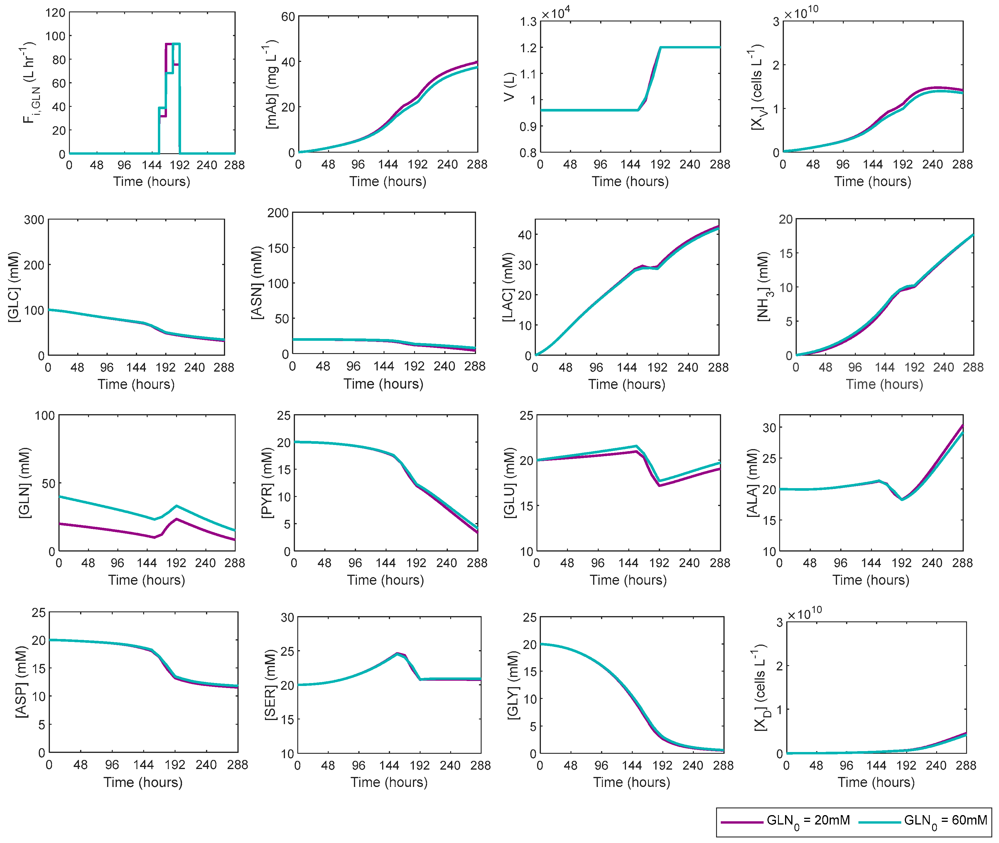
3.2. Glutamine Fed-Batch Dynamic Optimisations

Optimal trajectories for glutamine-fed bioreactor systems are depicted in Figure 5. Most of the glutamine fed-batch bioreactor optimal trajectories vary very slightly (if at all) between GLN_20mM and GLN_60mM cases. The optimal feeding strategies vary very slightly, with the GLN_20mM peak feed occurring 12 h before the GLN_60mM one. For both GLN_20mM and GLN_60mM cases, the entirety of feeding is complete between 156–192 h (days 6–8). The glutamate concentration is lower throughout the time domain for the GLN_20mM, compared to the GLN_60mM case, as it is directly proportional. Glutamine concentration levels differ clearly as expected between the cases, but all other signals show very small differences, in line with whether higher feed favours them or not. Moreover, and in line with the previous (GLC) observation, the GLN_20mM exhibited marginally larger final mAb titer and viable cell counts compared to the GLN_60mM case. The concentrations of toxic by-products (lactate, ammonia) are very similar for both cases.

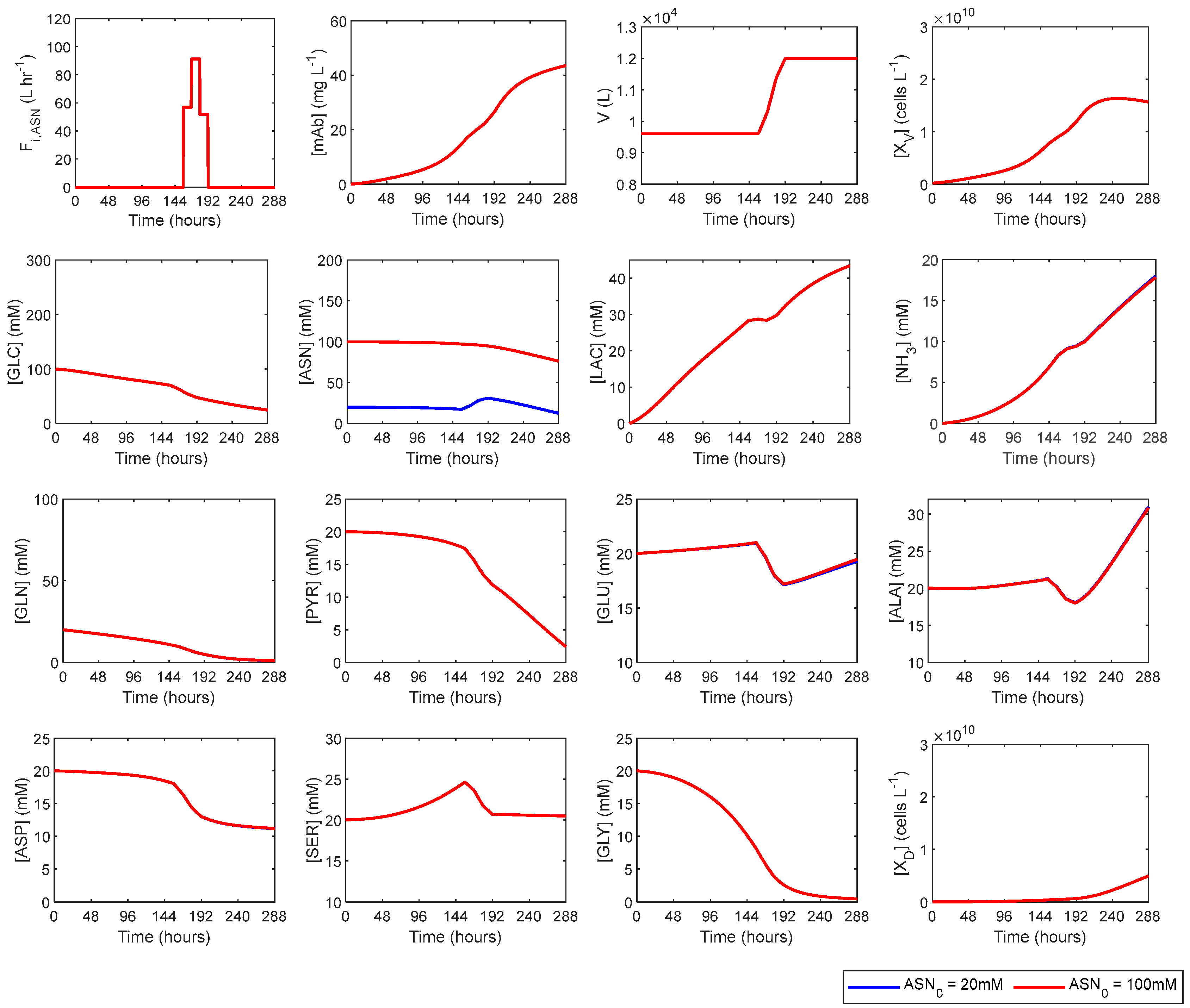
3.3. Asparagine Fed-Batch Dynamic Optimisations

Optimal trajectories for the asparagine-fed bioreactor systems are shown in Figure 6.

Because of the miniscule (if even observable) differences between both cases (runs 5–6), asparagine feed strategies have little, if any, effect: lines are virtually indistinguishable, as only asparagine and glutamate trajectories vary between ASN_20mM and ASN_100mM. As expected, asparagine concentration is greater in the case of ASN_100mM, and later stage (days 12–14) glutamate is slightly lower in the case of ASN_20mM, indicating that asparagine does contribute to glutamate regulation for its usage within the TCA cycle. Both asparagine fed-batch systems (runs 5–6) have exhibited improved mAb titers and viable cell counts compared to the glutamine systems (runs 3–4), although it is important to note that performance and productivity did not reach as much as was achieved in the glucose-fed bioreactor case of GLC_30mM (run) in terms of either of these two metrics.

An important remark emerges about fed-batch bioreactor sensitivity to nutrient feed strategy optimisation, when comparing results from runs 3–4 to 5–6: although glutamine and asparagine yield strikingly similar optimal profiles for most metabolites despite the level variation, the viable cell and product (mAb) levels may vary substantially—or not.

4. Discussion

Table 3. Summary of the final time viable cell counts and mAb titers.

Run	Initial Condition	${\mathit{X}}_{\mathit{V}}\left({\mathit{t}}_{\mathit{f}}\right)$ (Cells mL–1)	$\mathbf{Change} \mathbf{in} {\mathit{X}}_{\mathit{V}}\left({\mathit{t}}_{\mathit{f}}\right)$ (%)	$\mathit{m}\mathit{A}\mathit{b}\left({\mathit{t}}_{\mathit{f}}\right)$ (mg L–1)	$\mathbf{Change} \mathbf{in} \mathit{m}\mathit{A}\mathit{b}\left({\mathit{t}}_{\mathit{f}}\right)$ (%)
1	GLC_100mM	1.329 × 1010	-	35.73	-
2	GLC_30mM	1.905 × 1010	43.34	52.70	47.50
3	GLN_20mM	1.419 × 1010	6.77	39.68	11.06
4	GLN_60mM	1.353 × 1010	1.81	37.44	4.79
5	ASN_20mM	1.566 × 1010	17.83	43.58	21.97
6	ASN_100mM	1.566 × 1010	17.83	43.57	21.94

presents final-time values serving as key fed-batch bioreactor performance metrics (viable cell count and mAb titer) after a set time horizon (12 days of operation, runs 1–6), as well as their relative differences (percentage change) vs. the base case, GLC_100mM). The sensitivity analysis identifies GLC_100mM as the actually weakest of the 6 cases we have explored (as all other five runs 2–6, exhibit growth in viable cell count and mAb titer). The hypothesis that glucose over-supplementation may well lead to poor cultivation is confirmed: both key metrics benefit significantly from lower GLC content (GLC_30mM).

Both runs 3 and 4 exhibit rather minor improvements vs. the GLC_100mM base case. Nevertheless, the GLN_20mM case clearly provides superior amounts of final time viable cells (7%) and mAb titer (11%), vs. much more modest improvements for GLN_60mM. This finding shows that extra glutamine does not promote GS-CHO cell line performance.

The small mAb titer gains (1.8–11%) of GLN cases vs. the GLC_100mM base case and better culture performance with less initial glutamine imply that optimisation for the given GS-CHO culture need not consider glutamine feed flow manipulation as a priority.

Both runs 5 and 6 exhibit key (almost identical) improvements in both performance metrics, with viable cell count ca. 18% and mAb titer ca. 22% higher than the base case. Moreover, both ASN cases achieve higher improvements than those for GLN-fed designs, but neither run 5 nor 6 yield values as high as those seen in run 2 (glucose-restricted case).

5. Conclusions

Industrial scale fed-batch monoclonal antibody (mAbs) manufacturing by means of a mammalian GS-CHO is of extreme societal importance, to ensure provision of critical healthcare and advanced biotherapeutics to many millions of patients worldwide [1,2,3,4,5,6,7]. Accessibility and affordability of mAb therapies is strongly dependent on geographic as well as socioeconomic parameters [36], thus process intensification in biopharmaceutical manufacturing can have a pivotal impact on reducing enormous barriers to public health.

This computational study investigates the efficiency of several different substrate feeding strategies on GS-CHO culture health (viable cell count) and mAb yield (final titer). Single-objective dynamic optimisation has been implemented to maximise the final mAb mass at the termination of bioreactor operation (set after 12 days). A simultaneous method (orthogonal collocation on finite elements) has been used to formulate the NLP problems, and a robust, established NLP solver (IPOPT) [29] is applied for determining the optimal manipulated feeding strategies (piecewise linear time trajectories, using a 12-h time step).

Each bioreactor design is considered with identical initial and final working volume; three widely used substrates (glucose, glutamine, asparagine) are the manipulated feeds. To ensure that the effect of each individual (time-varying feed) substrate can be clearly understood after the dynamic optimisation of fed-batch bioreactor operation, we consider six (6) individual case studies, in which only one substrate can be fed during each run, although the set initial conditions for medium composition contain portions of all three. The time horizon (operation) is set at 12 days (288 h), while the time step for action (feed level change) is set at 12 h, to account for slow sensors or mixing imperfections.

This rather coarse time grid also reflects the implied practical limitations in regard to sampling and possible offline experimentation (instrumental analysis) that may be required to establish credible measurements, especially in lack of online (esp. real-time) PAT [15].

The proposed dynamic flux balance model is based on a recent combined study [27] and has been individually validated vs. both experimental data and simulation results of its original authors, Yilmaz et al., (2020), as demonstrated in detail in our Figure 3a,b: for certain dynamic state variables, and due to parameter value adjustments, our own model predictions (colour lines) are in better agreement with data vs. the earlier (black line) ones.

Our scope, given this reliable model, is to pinpoint efficient (and economical, in regard to feedstock use) substrate manipulations for production-scale technoeconomic evaluation.

The sensitivity analysis analyses final-time bioreactor performance metrics (Table 3) compiled from dynamic optimisation trajectory comparisons illustrated in Figure 4, Figure 5 and Figure 6, for the six case studies (two initial condition levels for each of the three substrates explored). Our major conclusion is that GS-CHO cells benefit from glucose reduction in the initial medium, since the GLC_30mM case is almost 50% more efficient than GLC_100mM one.

Glutamine has a markedly minor (almost insignificant role) in the manipulation of GS-CHO culture performance, as very small (ca. 10%) improvements can be achieved vs. the base-case; a three-fold increase of its concentration actually diminishes the gains achieved for high-glutamine (GLN_60mM) vs. the low-glutamine (GLN_20mM) scenario.

Our initial hypothesis is that the GS-CHO cell culture considered in the original [27] (therefore also in our) dynamic model will not need extra supplementation of glutamine, due to the amplification of the glutamine synthetase gene on the cell line investigated. This hypothesis appears plausible as per Figure 5 trajectories, since a three-fold GLN increase in initial medium composition only yields barely discernible metabolite changes, if at all.

Asparagine may well have a more important role in the later stage cell function, because dynamic optimisation results show that 20% improvements (almost independent of its initial load) can be achieved in both viable cell count and mAb titer vs. the base case. This performance improvement for ASN-fed cases implies that ASN has a more important role in cell proliferation and protein transcription than GLN does, in GS-CHO cell lines.

This observation suggests that asparagine (ASN) has a much stronger and pivotal involvement in key metabolic pathways, in contrast to glutamine (GLN), and may thus contribute to cultivation beyond being an alternative to GLN nitrogen and carbon donor. Clearly, initial asparagine conditions have a negligible effect on bioreactor performance, since runs 5–6 display identical optimal feeding strategies and state variable trajectories. Accordingly, we can reasonably conclude that initial asparagine levels in culture media may regulate late GS-CHO cells proliferation more efficiently than glucose ones. A higher asparagine concentration in the early stages of operation (or, even more so, its dynamic manipulation vs. initial medium content) cannot lead to tangible performance benefits.

The manipulation of glucose substrate levels is the most efficient for controlling mAb production, followed by asparagine, and then by glutamine dynamic level variation. Whilst there are clear correlations observed for the three individual substrates here, further sensitivity analyses can tackle dynamic feed manipulation of multiple substrates. Metabolic pathways consist of multiple metabolites, each contributing to many (different for each one) cell functions. Feeding multiple substrates simultaneously can yield insight into which of them are more (or less) critical in the different phases of culture lifecycle.

Moreover, we must emphasise that whilst the dynamic flux balance model has been validated for use in the dynamic optimisation and subsequent sensitivity analysis, experimental bioreactor studies must be conducted so as to corroborate these in silico findings. The original model developers computed parameter values as regression averages, using a simulated annealing algorithm which has minimised the sum of square residuals [27]. Whilst this approach is computationally reliable, another larger experimental dataset for the dynamic behavior of GS-CHO in fed-batch reactors with a wide variety of substrates and feeding strategies can increase model fidelity and reproducibility, for industrial use.

Artificial Intelligence (AI) and Machine Learning (ML) methodologies promise a lot to the latter end, due to the size (and the multi-dimensional uncertainty) of biopharma datasets. Such ML approaches are already investigated for continuous mAb manufacturing [37].

Economic Model-Predictive Control (eMPC) is another recently established idea [38] towards efficiently bridging dynamic process optimisation and technoeconomic evaluation via an integrated framework: therein, the economic performance objective (e.g., max. profit) can effectively replace the simpler (mAb titer) one used here, while also hosting cost data, all foregoing (technical) constraints, and even more. The latter may e.g., include a more realistic representation of actual bioreactor operation, via input rate-of-change constraints, to limit input variation (e.g., sudden/abrupt feed jumps) between sampling and actuation time points. Such derivative constraints portray key practical limitations. Employing optimized feed trajectories in feedback mode in an eMPC framework requires adequate biological uncertainty characterisation, but also explicit account of time delays.

References

1. Chames, P.; Van Regenmortel, M.; Weiss, E.; Baty, D. Therapeutic antibodies: Successes, limitations and hopes for the future. Br. J. Pharmacol. 2009, 157, 220–233. [Google Scholar] [CrossRef]
2. Mahmuda, A.; Bande, F.; Al-Zihiry, K.J.K.; Abdulhaleem, N.; Majid, R.A.; Hamat, R.A.; Abdullah, W.O.; Unyah, Z. Monoclonal antibodies: A review of therapeutic applications and future prospects. Trop. J. Pharm. Res. 2017, 16, 713–722. [Google Scholar] [CrossRef]
3. Dhara, V.G.; Naik, H.M.; Majewska, N.I.; Betenbaugh, M.J. Recombinant antibody production in CHO and NS0 cells: Differences and similarities. BioDrugs 2018, 32, 571–584. [Google Scholar] [CrossRef]
4. Jain, E.; Kumar, A. Upstream processes in antibody production: Evaluation of critical parameters. Biotechnol. Adv. 2008, 26, 46–72. [Google Scholar] [CrossRef]
5. Liu, J.K. The history of monoclonal antibody development—Progress, remaining challenges and future innovations. Ann. Med. Surg. 2014, 3, 113–116. [Google Scholar] [CrossRef]
6. Lu, R.-M.; Hwang, Y.-C.; Liu, I.-J.; Lee, C.-C.; Tsai, H.-Z.; Li, H.-J.; Wu, H.-C. Development of therapeutic antibodies for the treatment of diseases. J. Biomed. Sci. 2020, 27, 1–30. [Google Scholar] [CrossRef] [PubMed]
7. Grilo, A.L.; Mantalaris, A. The increasingly human and profitable monoclonal antibody market. Trends Biotechnol. 2019, 37, 9–16. [Google Scholar] [CrossRef]
8. Kastelic, M.; Kopač, D.; Novak, U.; Likozar, B. Dynamic metabolic network modeling of mammalian Chinese hamster ovary (CHO) cell cultures with continuous phase kinetics transitions. Biochem. Eng. J. 2019, 142, 124–134. [Google Scholar] [CrossRef]
9. Kirsch, B.J.; Bennun, S.V.; Mendez, A.A.; Johnson, A.S.; Wang, H.; Qiu, H.; Li, N.; Lawrence, S.M.; Bak, H.; Betenbaugh, M.J. Metabolic analysis of the asparagine and glutamine dynamics in an industrial Chinese hamster ovary fed-batch process. Biotechnol. Bioeng. 2022, 119, 807–819. [Google Scholar] [CrossRef]
10. Kontoravdi, C.; Pistikopoulos, E.N.; Mantalaris, A. Systematic development of predictive mathematical models for animal cell cultures. Comput. Chem. Eng. 2010, 34, 1192–1198. [Google Scholar] [CrossRef]
11. Kiparissides, A.; Georgakis, C.; Mantalaris, A.; Pistikopoulos, E.N. Design of in silico experiments as a tool for nonlinear sensitivity analysis of knowledge-driven models. Ind. Eng. Chem. Res. 2014, 53, 7517–7525. [Google Scholar] [CrossRef]
12. Kiparissides, A.; Pistikopoulos, E.N.; Mantalaris, A. On the model-based optimization of secreting mammalian cell (GS-NS0) cultures. Biotechnol. Bioeng. 2015, 112, 536–548. [Google Scholar] [CrossRef] [PubMed]
13. Kelley, B.; Renshaw, T.; Kamarck, M. Process and operations strategies to enable global access to antibody therapies. Biotechnol. Prog. 2021, 37, e3139. [Google Scholar] [CrossRef] [PubMed]
14. Lohmann, L.J.; Strube, J. Accelerating biologics manufacturing by modeling: Process integration of precipitation in mAb downstream processing. Processes 2020, 8, 58. [Google Scholar] [CrossRef]
15. Lohmann, L.J.; Strube, J. Process Analytical Technology for precipitation process integration into biologics manufacturing towards autonomous operation: mAb case study. Processes 2021, 9, 488. [Google Scholar] [CrossRef]
16. Jones, W.; Gerogiorgis, D.I. Parametric analysis of mammalian cell (GS-NS0) culture performance for advanced mAb biopharmaceutical manufacturing. Comp. Aid. Chem. Eng. 2021, 50, 1923–1928. [Google Scholar]
17. Jones, W.; Gerogiorgis, D.I. Dynamic optimisation and comparative analysis of fed-batch and perfusion bioreactor performance for monoclonal antibody (mAb) manufacturing. Comp. Aid. Chem. Eng. 2022, 51, 1117–1122. [Google Scholar]
18. Jones, W.; Gerogiorgis, D.I. Dynamic simulation, optimisation and economic analysis of fed-batch vs. perfusion bioreactors for advanced mAb manufacturing. Comput. Chem. Eng. 2022, 165, 107855. [Google Scholar]
19. Varadaraju, H.; Schneiderman, S.; Zhang, L.; Fong, H.; Menkhaus, T.J. Process and economic evaluation for monoclonal antibody purification using a membrane-only process. Biotechnol. Prog. 2011, 27, 1297–1305. [Google Scholar] [CrossRef]
20. Mir-Artigues, P.; Twyman, R.M.; Alvarez, D.; Cerda Bennasser, P.; Balcells, M.; Christou, P.; Capell, T. A simplified techno-economic model for the molecular pharming of antibodies. Biotechnol. Bioeng. 2019, 116, 2526–2539. [Google Scholar] [CrossRef]
21. Gupta, P.; Kateja, N.; Mishra, S.; Kaur, H.; Rathore, A.S. Economic assessment of continuous processing for manufacturing of biotherapeutics. Biotechnol. Prog. 2021, 37, e3108. [Google Scholar] [CrossRef]
22. Gerogiorgis, D.I.; Barton, P.I. Steady-state optimization of a continuous pharmaceutical process. Comp. Aid. Chem. Eng. 2009, 27, 927–932. [Google Scholar]
23. Rodman, A.D.; Gerogiorgis, D.I. Dynamic optimization of beer fermentation: Sensitivity analysis of attainable performance vs. product flavour constraints. Comput. Chem. Eng. 2017, 106, 582–595. [Google Scholar] [CrossRef]
24. Rodman, A.D.; Fraga, E.S.; Gerogiorgis, D.I. On the application of a nature-inspired stochastic evolutionary algorithm to constrained multi-objective beer fermentation. Comput. Chem. Eng. 2018, 108, 448–459. [Google Scholar] [CrossRef]
25. Shirahata, H.; Diab, S.; Sugiyama, H.; Gerogiorgis, D.I. Dynamic modelling, simulation and economic evaluation of two CHO cell-based production modes towards developing biopharmaceutical manufacturing processes. Chem. Eng. Res. Des. 2019, 150, 218–233. [Google Scholar] [CrossRef]
26. Botelho Ferreira, K.; Benlegrimet, A.; Diane, G.; Pasquier, V.; Guillot, R.; De Poli, M.; Chappuis, L.; Vishwanathan, N.; Souquet, J.; Broly, H.; et al. Transfer of continuous manufacturing process principles for mAb production in a GMP environment: A step in the transition from batch to continuous. Biotechnol. Prog. 2022, 38, e3259. [Google Scholar] [CrossRef] [PubMed]
27. Yilmaz, D.; Parulekar, S.J.; Cinar, A. A dynamic EFM-based model for antibody producing cell lines and model based evaluation of fed-batch processes. Biochem. Eng. J. 2020, 156, 107494. [Google Scholar] [CrossRef]
28. Biegler, L.T. Solution of dynamic optimization problems by successive quadratic programming and orthogonal collocation. Comput. Chem. Eng. 1984, 8, 243–247. [Google Scholar] [CrossRef]
29. Wächter, A.; Biegler, L.T. On the implementation of an interior-point filter line-search algorithm for large-scale nonlinear programming. Math. Program. 2006, 106, 25–57. [Google Scholar] [CrossRef]
30. Hedengren, J.D.; Shishavan, R.A.; Powell, K.M.; Edgar, T.F. Nonlinear modeling, estimation and predictive control in APMonitor. Comput. Chem. Eng. 2014, 70, 133–148. [Google Scholar] [CrossRef]
31. Fan, Y.; Jimenez Del Val, I.; Müller, C.; Sen, J.W.; Rasmussen, S.K.; Kontoravdi, C.; Weilguny, D.; Andersen, M.R. Amino acid and glucose metabolism in fed-batch CHO cell culture affects antibody production and glycosylation. Biotechnol. Bioeng. 2015, 112, 521–535. [Google Scholar] [CrossRef]
32. Zhou, W.; Chen, C.C.; Buckland, B.; Aunins, J. Fed-batch culture of recombinant NS0 myeloma cells with high monoclonal antibody production. Biotechnol. Bioeng. 1997, 55, 783–792. [Google Scholar] [CrossRef]
33. Mason, G.F.; Gruetter, R.; Rothman, D.L.; Behar, K.L.; Shulman, R.G.; Novotny, E.J. Simultaneous determination of the rates of the TCA cycle, glucose utilization, α-ketoglutarate/glutamate exchange, and glutamine synthesis in human brain by NMR. J. Cereb. Blood Flow Metab. 1995, 15, 12–25. [Google Scholar] [CrossRef]
34. Farid, S.S. Process economics of industrial monoclonal antibody manufacture. J. Chromatogr. B 2007, 848, 8–18. [Google Scholar] [CrossRef]
35. Kappatou, C.D.; Mhamdi, A.; Campano, A.Q.; Mantalaris, A.; Mitsos, A. Model-based dynamic optimization of monoclonal antibodies production in semibatch operation—Use of reformulation techniques. Ind. Eng. Chem. Res. 2018, 57, 9915–9924. [Google Scholar] [CrossRef]
36. Tong, X.; Li, X.; Pratt, N.L.; Hillen, J.B.; Stanford, T.; Ward, M.; Roughead, E.E.; Lai, E.C.-C.; Shin, J.-Y.; Cheng, F.W.; et al. Monoclonal antibodies and Fc-fusion protein biologic medicines: A multinational cross-sectional investigation of accessibility and affordability in Asia Pacific regions between 2010 and 2020. Lancet Reg. Health (West. Pac.) 2022, 26, 100506. [Google Scholar] [CrossRef]
37. Nikita, S.; Thakur, G.; Jesubalan, N.G.; Kulkarni, A.; Yezhuvath, V.B.; Rathore, A.S. AI-ML applications in bioprocessing: ML as an enabler of real time quality prediction in continuous manufacturing of mAbs. Comput. Chem. Eng. 2022, 164, 107896. [Google Scholar] [CrossRef]
38. Ellis, M.; Durand, H.; Christofides, P.D. A tutorial review of economic model predictive control methods. J. Proc. Control 2014, 8, 1156–1178. [Google Scholar] [CrossRef]
Figure 1. The total mAb market value and its significant rise over the recent years [7].
Processes 11 03065 g001
Figure 2. Fed-batch bioreactor operation for the production of monoclonal antibodies (mAbs).
Processes 11 03065 g002
Figure 3. Dynamic simulations of: (a) glutamine-rich and (b) glutamine-depleted batch reactor experiments.
Processes 11 03065 g003
Figure 4. Optimised GLC-fed FB bioreactors (runs 1 and 2).
Processes 11 03065 g004
Figure 5. Optimised GLN-fed FB bioreactors (runs 3 and 4).
Processes 11 03065 g005
Figure 6. Optimised ASN-fed FB bioreactors (runs 5 and 6).
Processes 11 03065 g006