
Research on the Heat Extraction Performance Optimization of Spiral Fin Coaxial Borehole Heat Exchanger Based on GA–BPNN–QLMPA

Abstract
:1. Introduction
2. Numerical Model and Validation
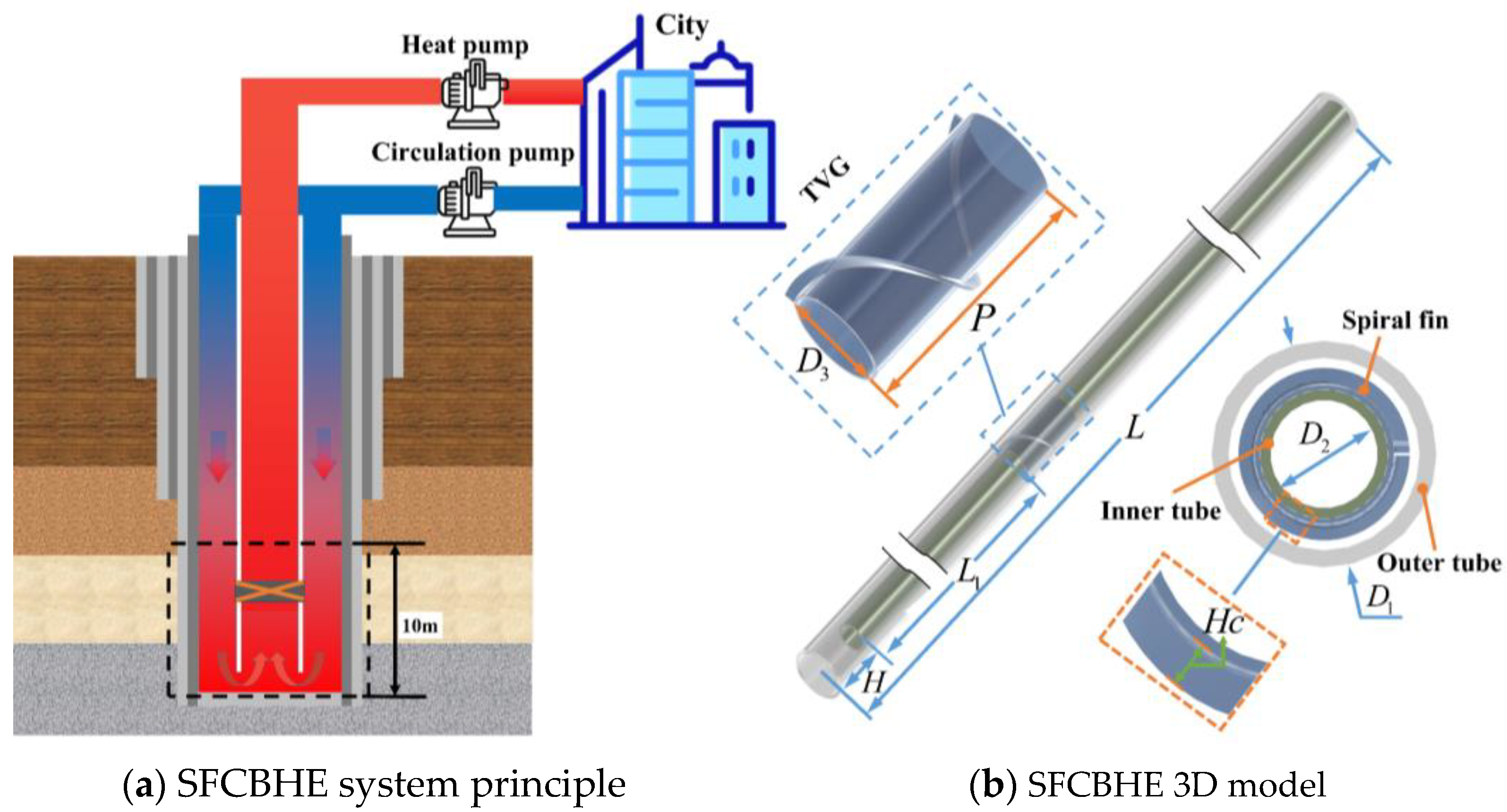
2.1. Geometric Model
2.2. Numerical Model and Evaluation Indicator
2.2.1. Model Assumption
- (1)
- The geotechnical soil around the geothermal well is assumed to be a homogeneous medium, groundwater seepage is neglected, and the heat transfer in the underground geotechnical soil is considered pure heat conduction.
- (2)
- The heat source at the well’s bottom and the surface temperature are considered constant.
- (3)
- The geotechnical soil’s surface temperature and thermophysical parameters change only along the depth direction.
- (4)
- It is assumed that the buried pipe, the backfill material, and the ground are closed in contact and that there is no contact thermal resistance between them.
2.2.2. Control Equations and Boundary Conditions
- (1)
- Control Models
- (2)
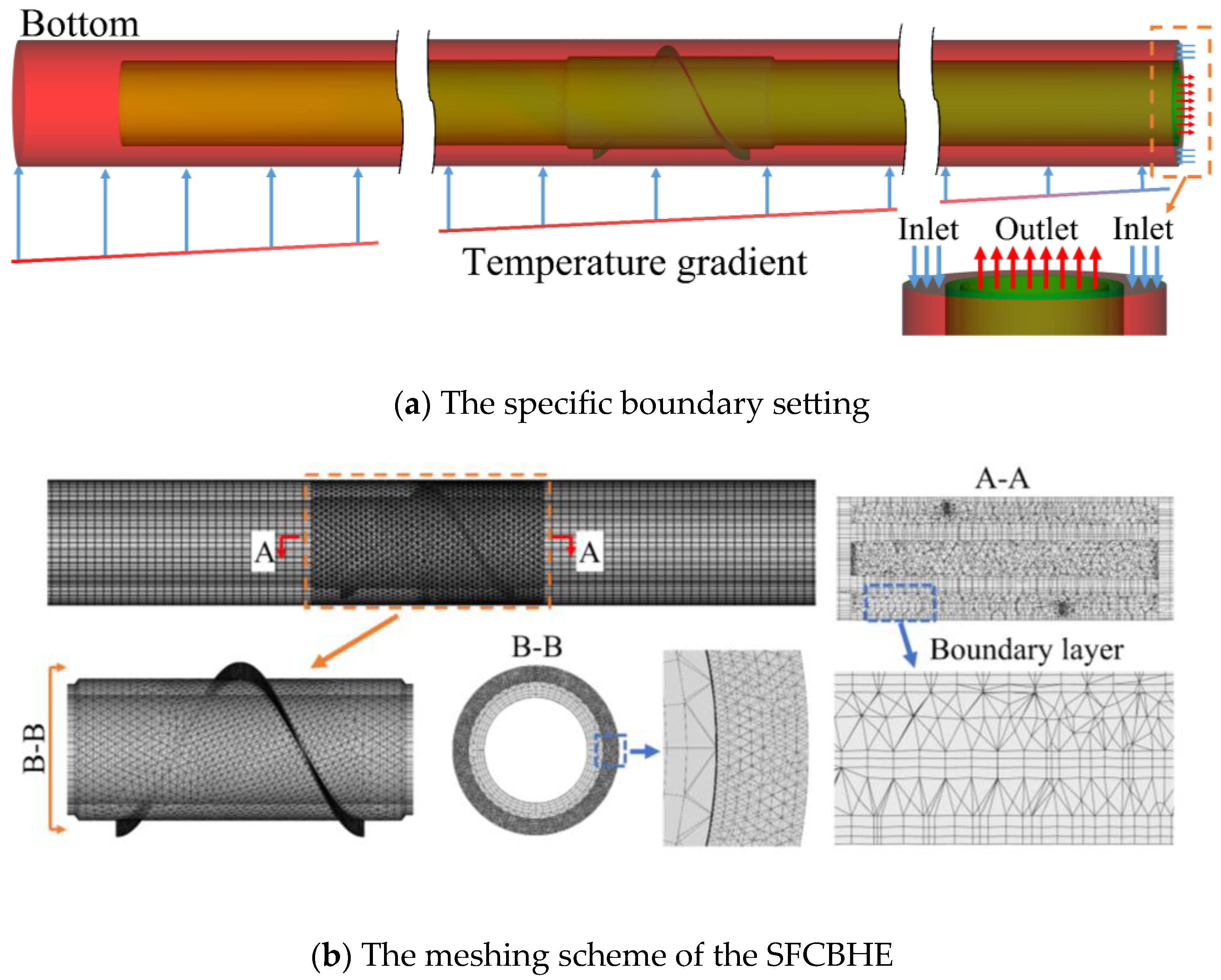
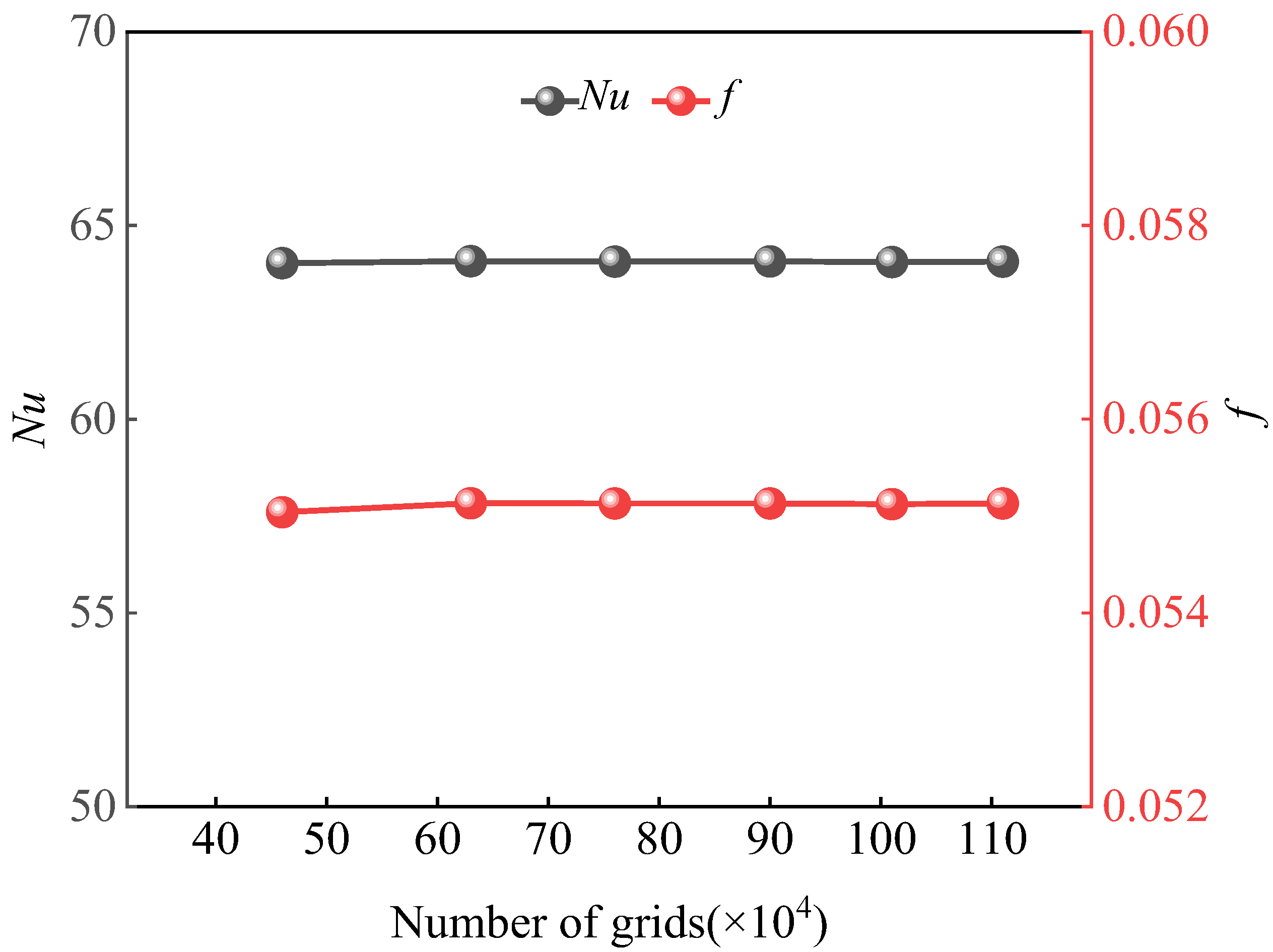
- Boundary conditions and meshing
- (1)
- Rock temperaturewhere TW is the rock temperature, K; Tsur is the ground surface temperature, K; Tg is the land temperature gradient, K/m; z is the well depth, m.
- (2)
- Outlet pressure
- (3)
- Physical parameters
2.2.3. Evaluation Indicator
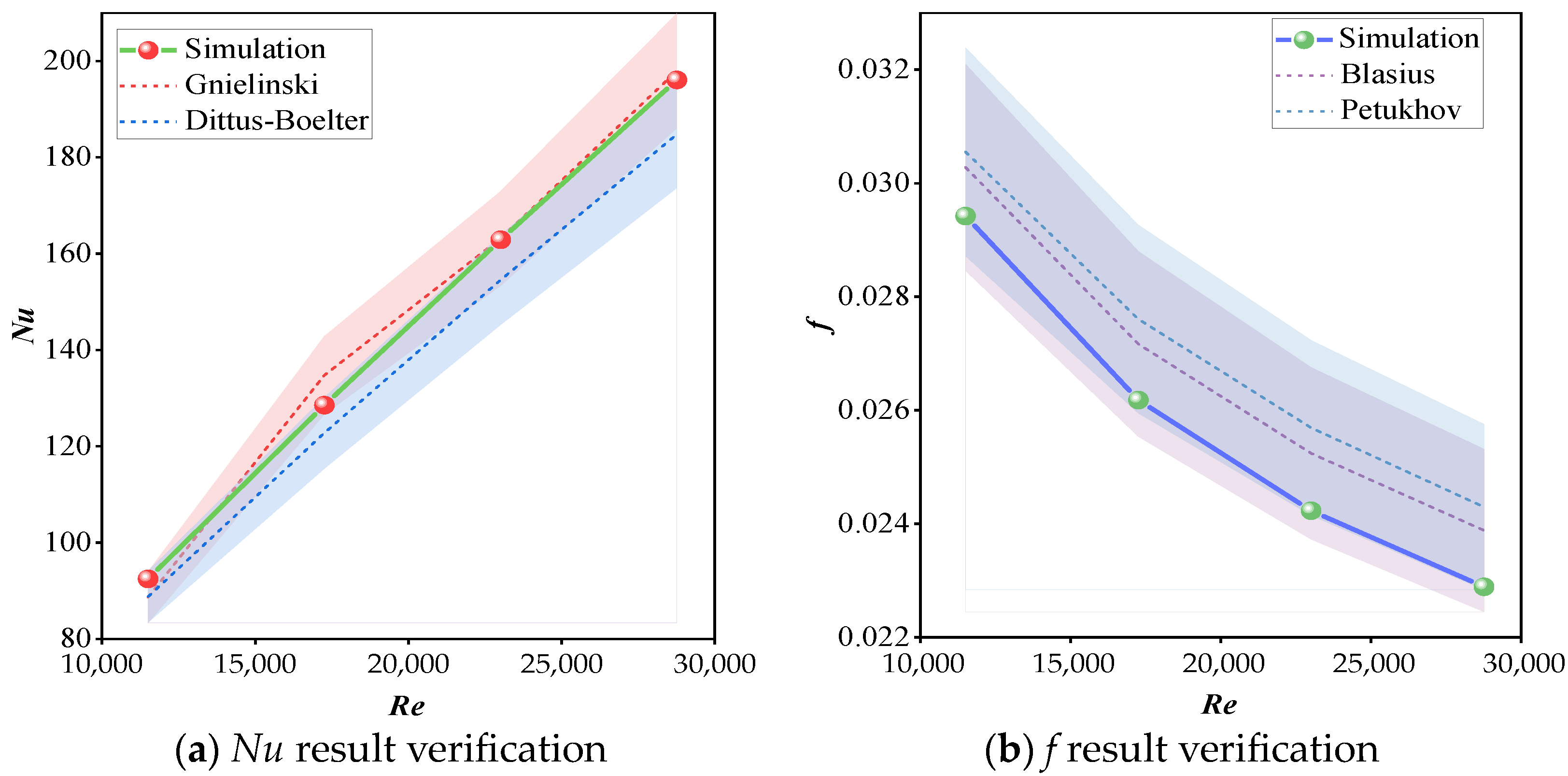
2.3. Model Validation
2.4. Taguchi Method Program
3. Optimization Models and Methods
3.1. PEC Optimization Model
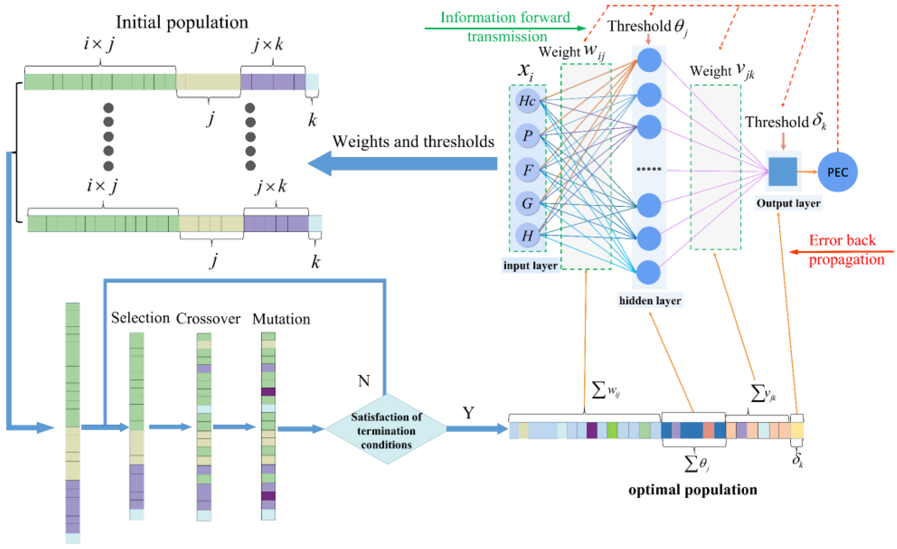
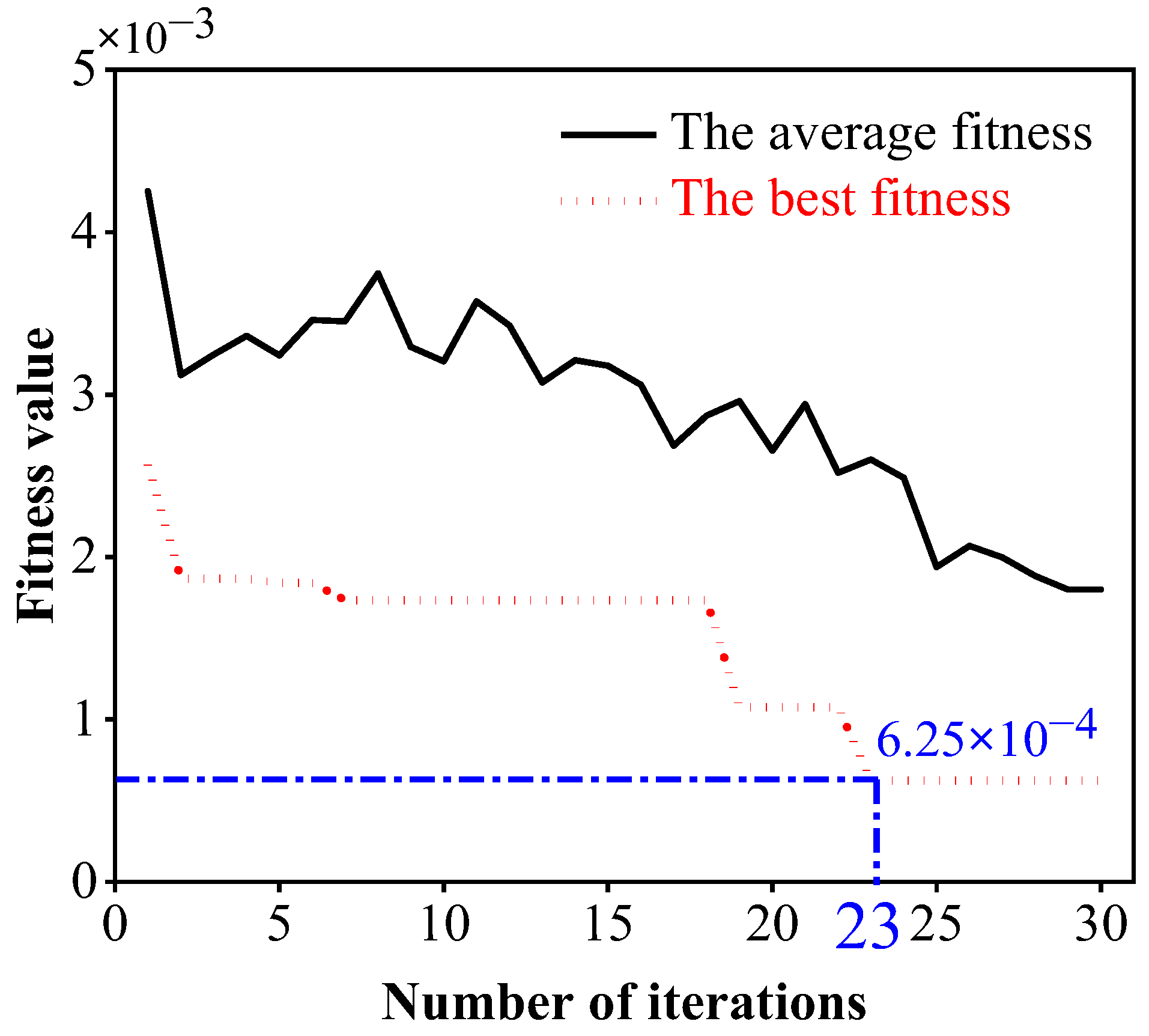
3.2. GA–BPNN Principles and Processes
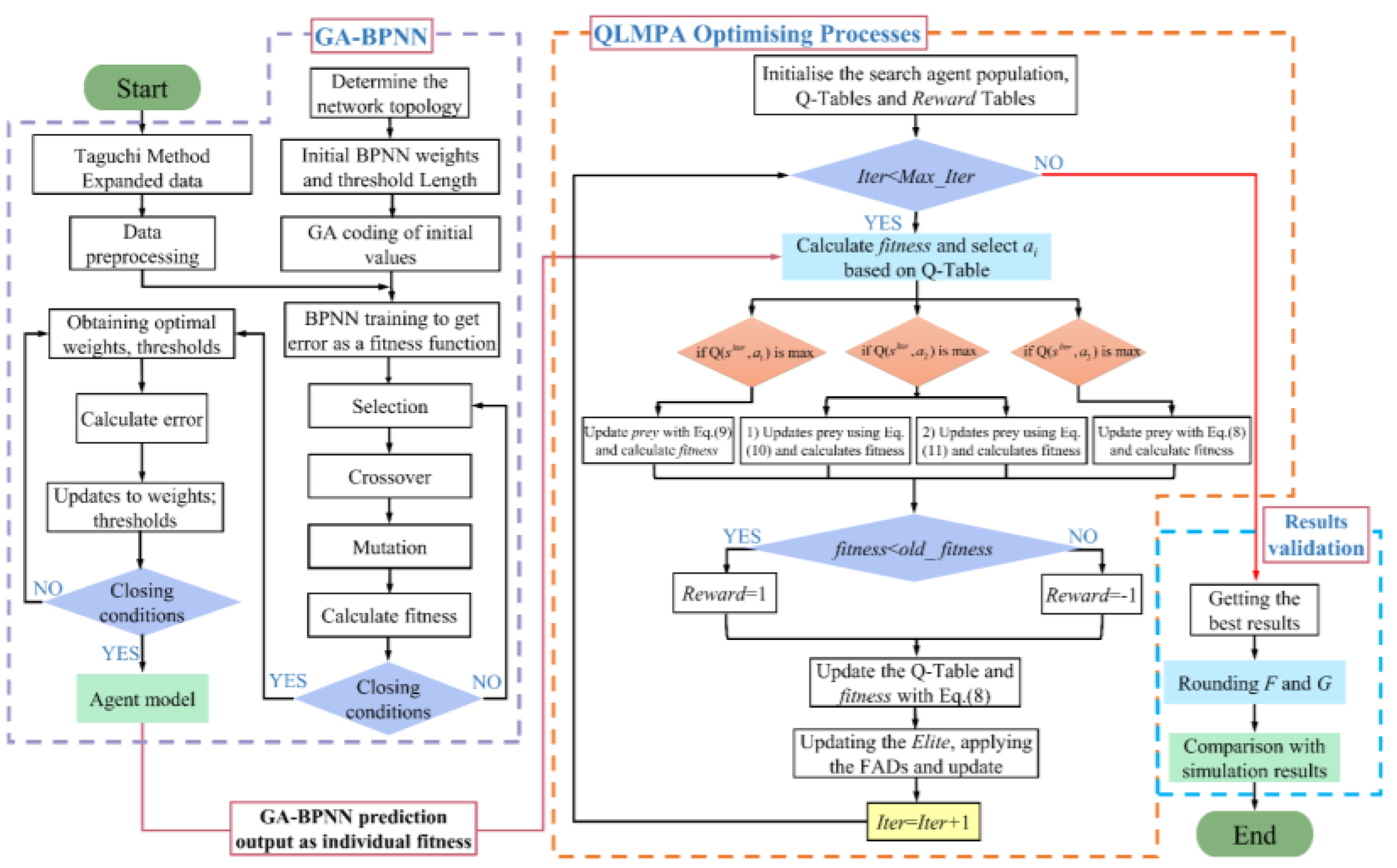
3.3. QLMPA Optimization Principles and Processes
- (1)
- Initialize the search agent (Preyi) population i = 1,…, n, Q-table, and Reward table, as well as the current state s0;
- (2)
- When the number of iterations is less than the maximum, the trained GA–BPNN prediction output is used as old_ fitness. The Elite matrix is constructed;
- (3)
- If Q(SIter,a1) is the maximum value in the Q-table, which is the initial phase of optimization, the predator moves faster than the prey, and Prey is updated using the following equation:where RB is a vector of random numbers containing the Brownian motion normal distribution; the symbol ⨂ denotes term-by-term multiplication; P is a constant, taken as 0.5; and R is a vector of uniform random numbers in the interval 0~1.
- (4)
- If Q(SIter,a2) is the maximum value in the Q-table, this is an optimized intermediate stage where the predator moves at a speed equal to the prey, and the setting is designed to be half for exploration and half for exploitation. For the exploration part of the population, Prey is updated according to Equation (10);where RL is a vector of random numbers with Le’vy distribution.
- (5)
- If Q(SIter,a3) is the maximum value in the Q-table, this is the final stage of optimization, and Prey is updated using the following equation:where simulates the predator Lev’y flight motion. Other factors influence the predator behavior, with eddy currents and fish aggregating devices (FADs) effects being the most significant [39,40].
- (6)
- Calculate fitness based on Prey; if fitness < old_ fitness, Reward = 1, otherwise, Reward = −1;
- (7)
- Update the Q-table with Equation (8), complete the Elite update, apply the FADs effect and update;
- (8)
- Add one to the number of iterations and go back to step 2;
- (9)
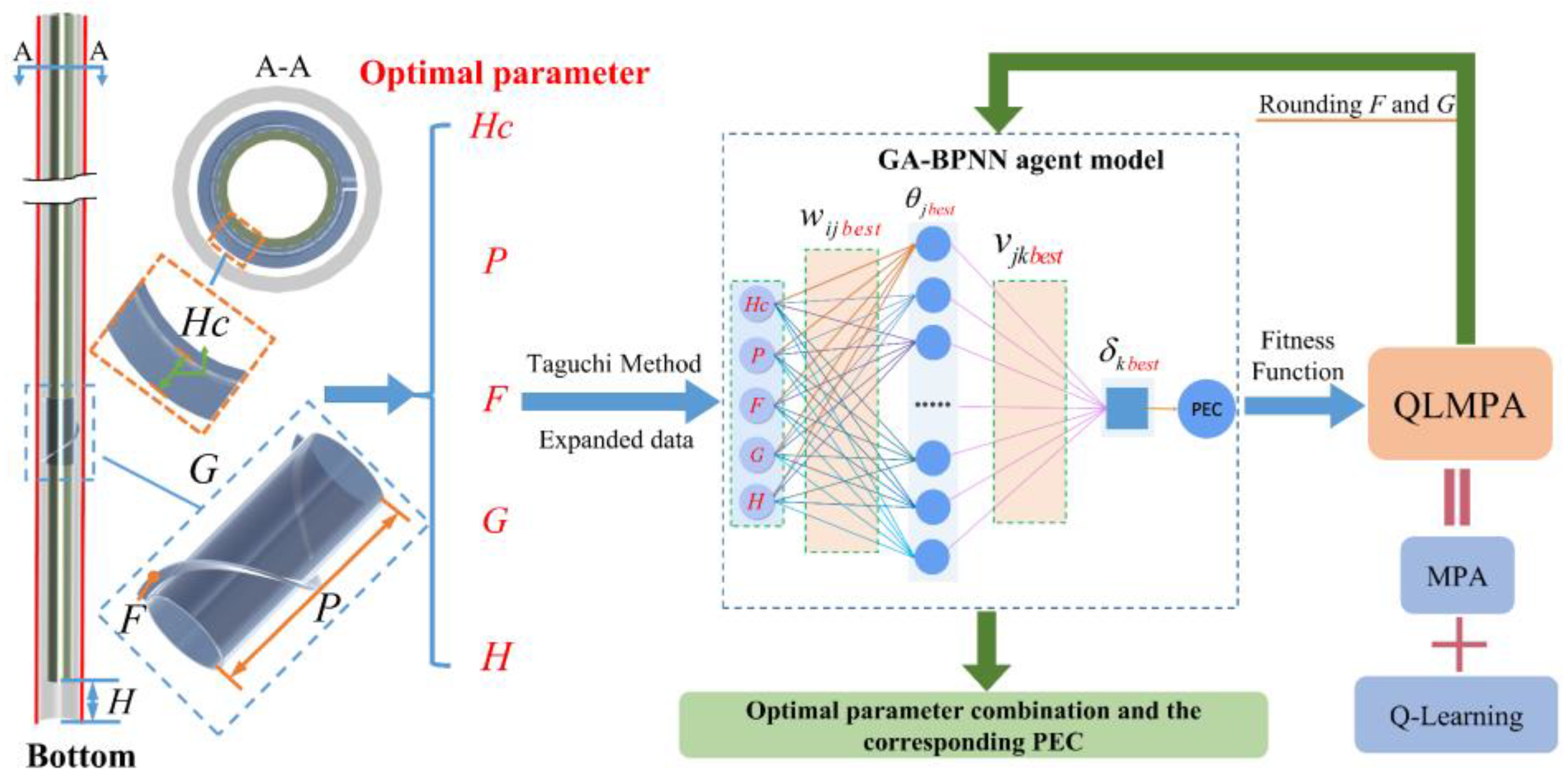
- At the end of the iteration, the best fitness and its corresponding Prey are returned. fitness is the optimal PEC obtained with QLMPA, and Prey is the optimal value of SFCBHE optimization variables (Hc, P, F, G, H);
- (10)
- The number of fins F and the number of vortex generators G in the optimal optimization variables obtained in step 9 are circularly substituted into the trained PEC agent model to find the PEC values;
- (11)
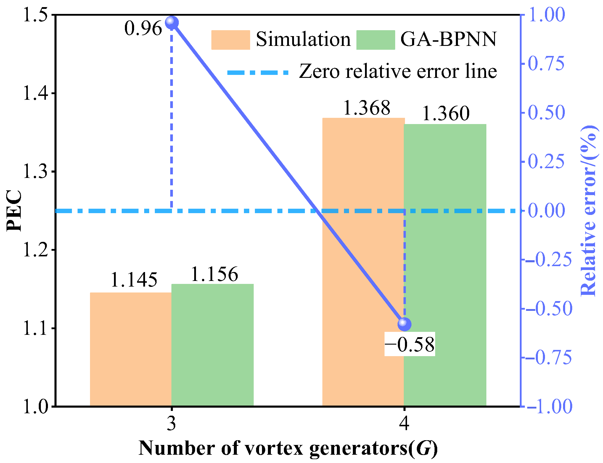
- Compare the results of the parameter combinations obtained in step 10 with the simulation analysis results to evaluate the optimized model’s accuracy.
4. PEC Prediction Model and Optimization Analysis
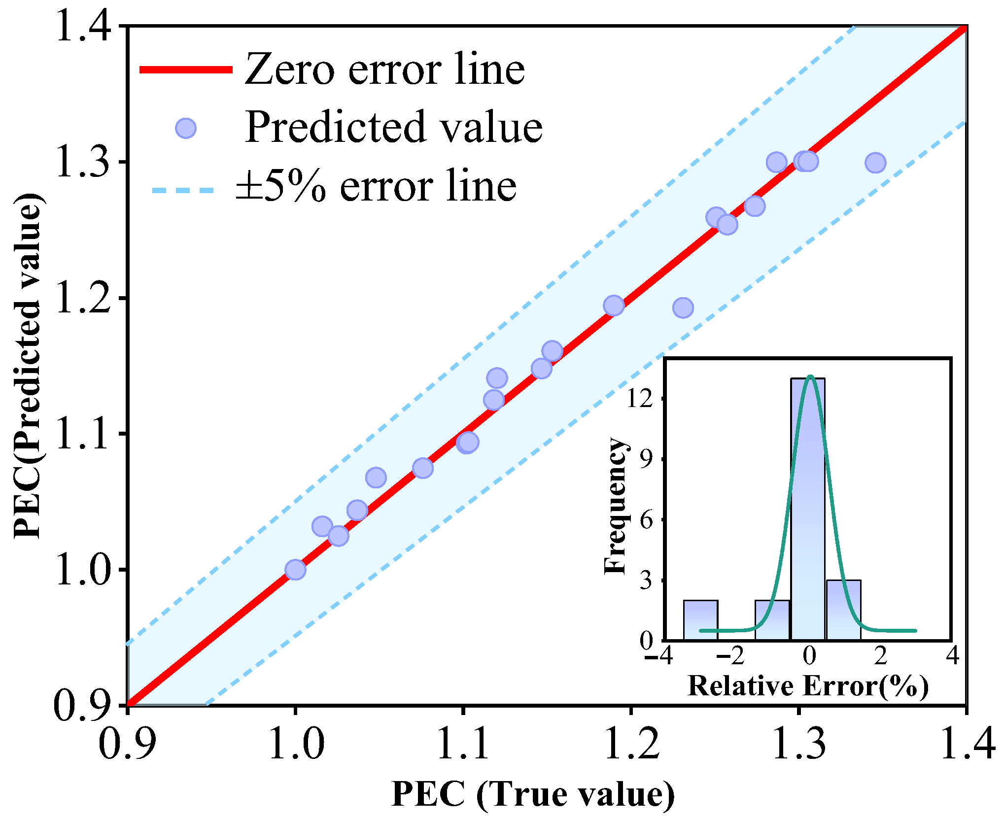
4.1. PEC Prediction Model
- (1)
- Test set prediction accuracy
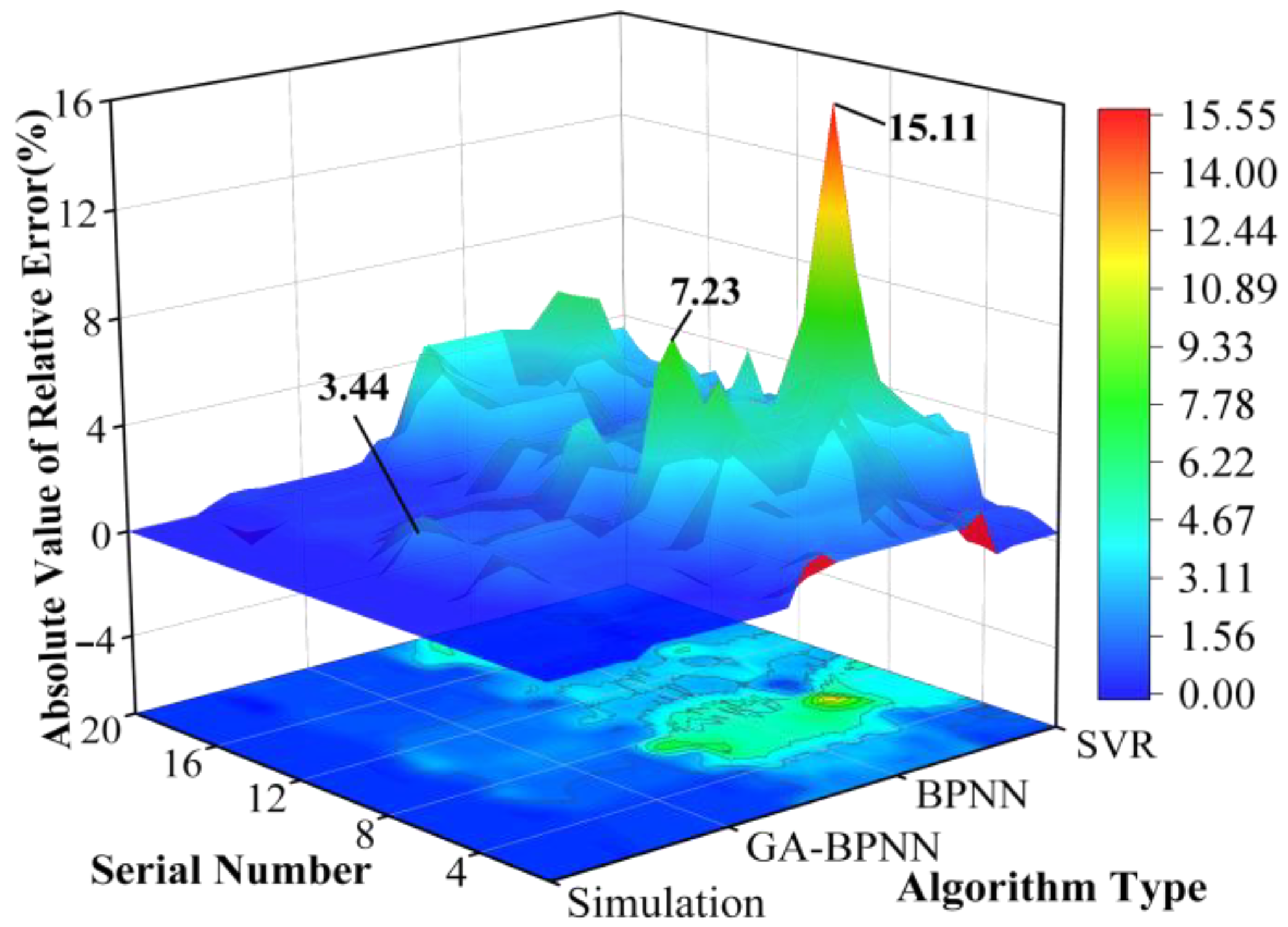
- (2)
- Error analysis
4.2. PEC Optimization Analysis
4.2.1. SFCBHE Parameter Optimization Results
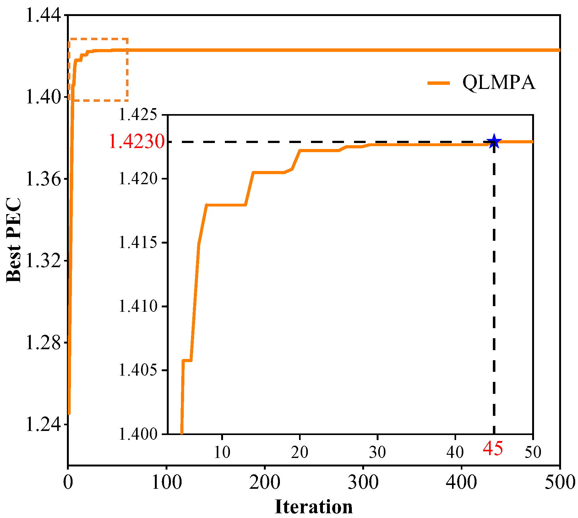
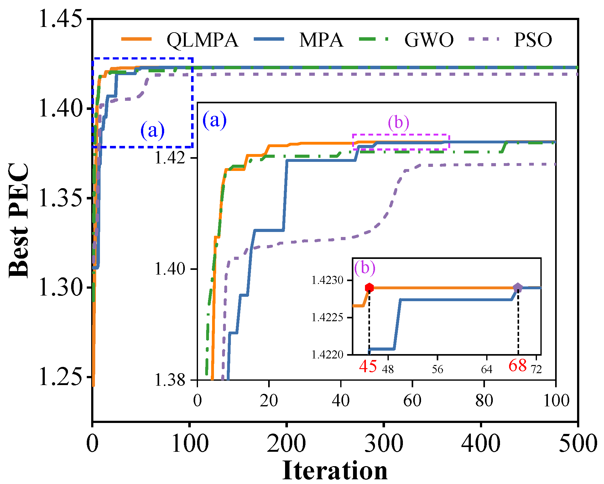
4.2.2. QLMPA Optimization Performance Evaluation
5. Optimized SFCBHE Heat Extraction Analysis
5.1. Heat Extraction Performance Comparison before and after Optimization
5.2. Heating Effect Assessment before and after Optimization
6. Conclusions
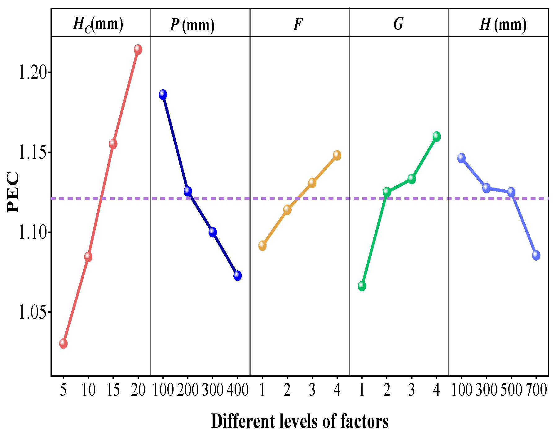
- (1)
- Orthogonal test and principal effect analysis were used to analyze the influence of main structural parameters on PEC. The results show that the degree of their influences was as follows: the fin height Hc > pitch P > number of vortex generators G > the distance of the lower end of the inlet tube from the bottom of the well H > number of fins F.
- (2)
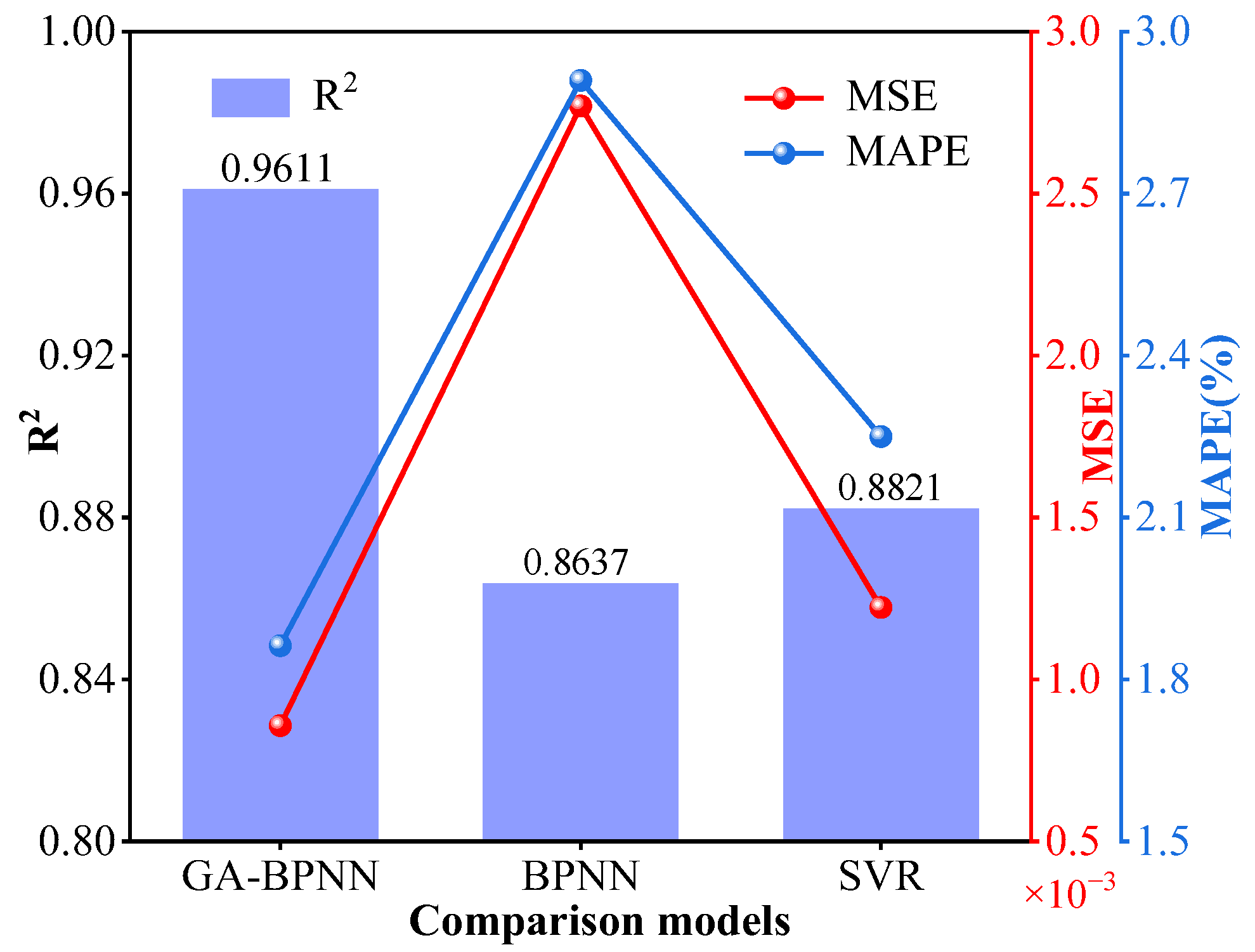
- The PEC prediction model is constructed using GA–BPNN, its prediction accuracy is 96.11%, which is 11.28% and 8.96% higher than that of the BPNN and SVR, respectively.
- (3)
- A fast design method is proposed for the SFCBHE based on the intelligence algorithm GA-BPNN-QLMPA. The PEC of the optimized SFCBHE is 1.36, it has been enhanced by 30.8% compared with traditional CBHE. The heat recovery performance of the optimized SFCBHE has been greatly improved.
- (4)
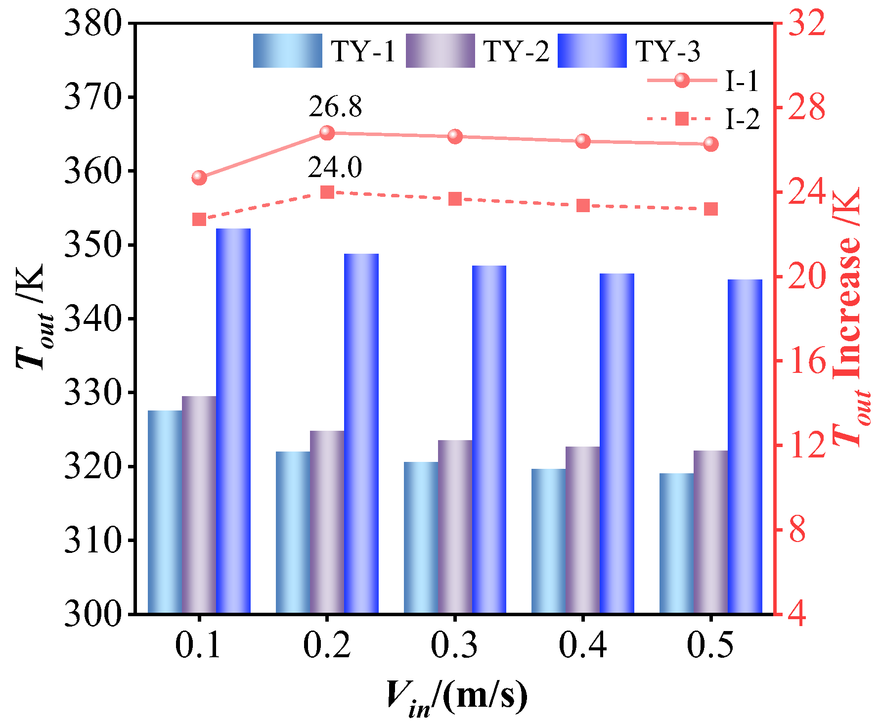
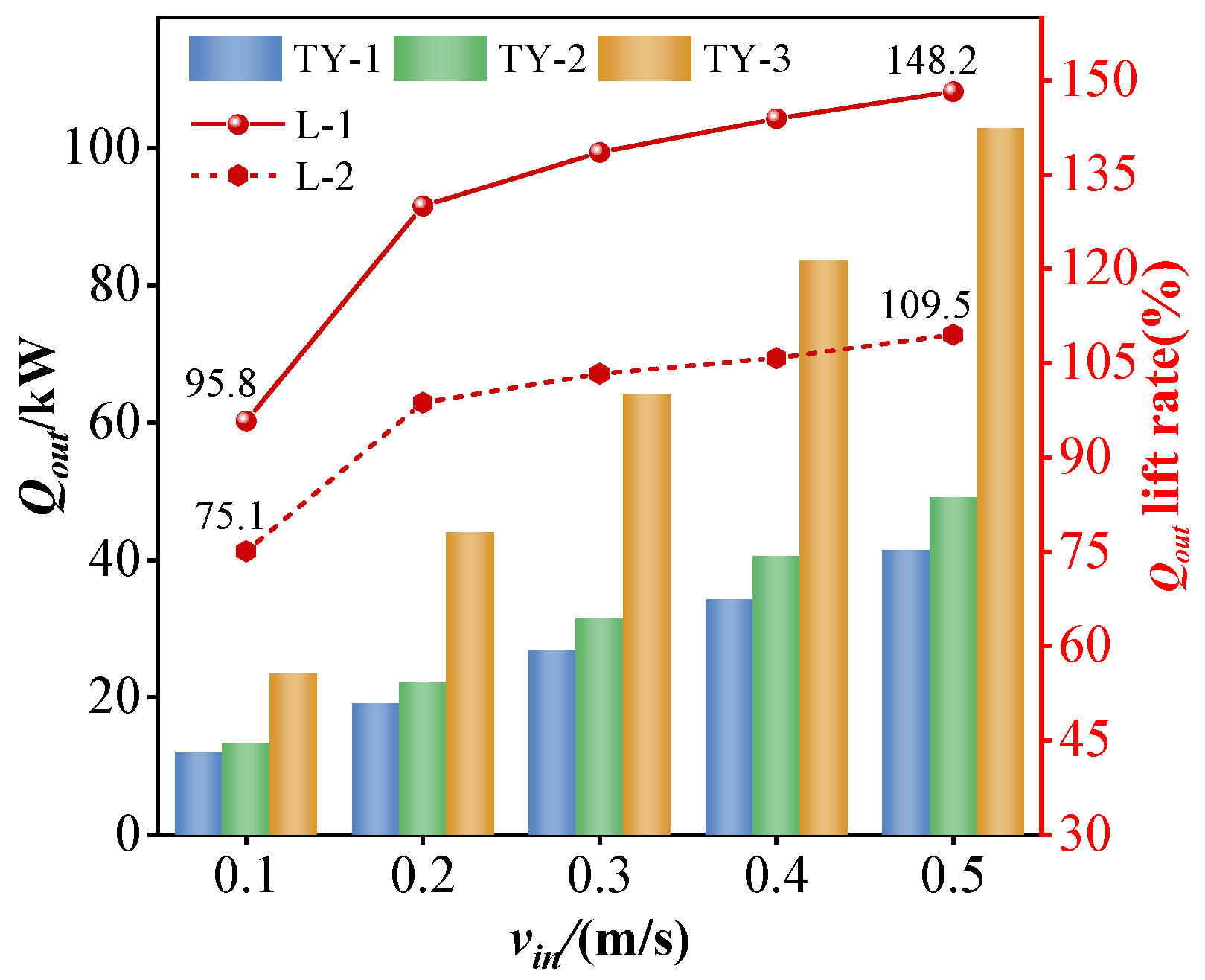
- When the flow rate is 0.2 m/s, the optimized SFCBHE has the highest extracted temperature, which is increased by 26.8 K compared to the smooth tube and 24.0 K compared to the pre-optimized SFCBHE. When the flow rate is 0.5 m/s, the optimized SFCBHE has the highest extracted power 102.8 kW, which is increased by 148.2% and 109.5% compared to the smooth pipe and the pre-optimized SFCBHE, respectively. Therefore, it is crucial to consider the extraction temperature and heat extraction power to determine the injection flow rate to achieve the optimal heat extraction.
Author Contributions
Funding
Data Availability Statement
Acknowledgments
Conflicts of Interest
Nomenclature
| SFCBHE | Spiral fin coaxial borehole heat exchanger |
| PEC | performance evaluation factor |
| GA-BPNN | gen-etic algorithm–back-propagation neural network |
| QLMPA | Q-learning-based marine predator algorithm |
| CBHE | coaxial borehole heat exchanger |
| BHE | borehole heat exchanger |
| DOTVG | the distance of the vortex generator from the bottom of the inner tube |
| TL | the total length of SFCBHE |
| OTD | the outer tube diameter |
| ITI | the insulation tube inner diameter |
| TVGD | the vortex generator’s diameter |
| TW | the rock temperature, K |
| Tsur | the ground surface temperature, K |
| Tg | the land temperature gradient, K/m |
| z | the well depth, m |
| Hc | fin height |
| P | pitch |
| F | number of fins |
| G | the number of vortex generators (uniform arrangement) |
| TDIT(H) | the distance of the lower end of the inlet tube from the bottom of the well |
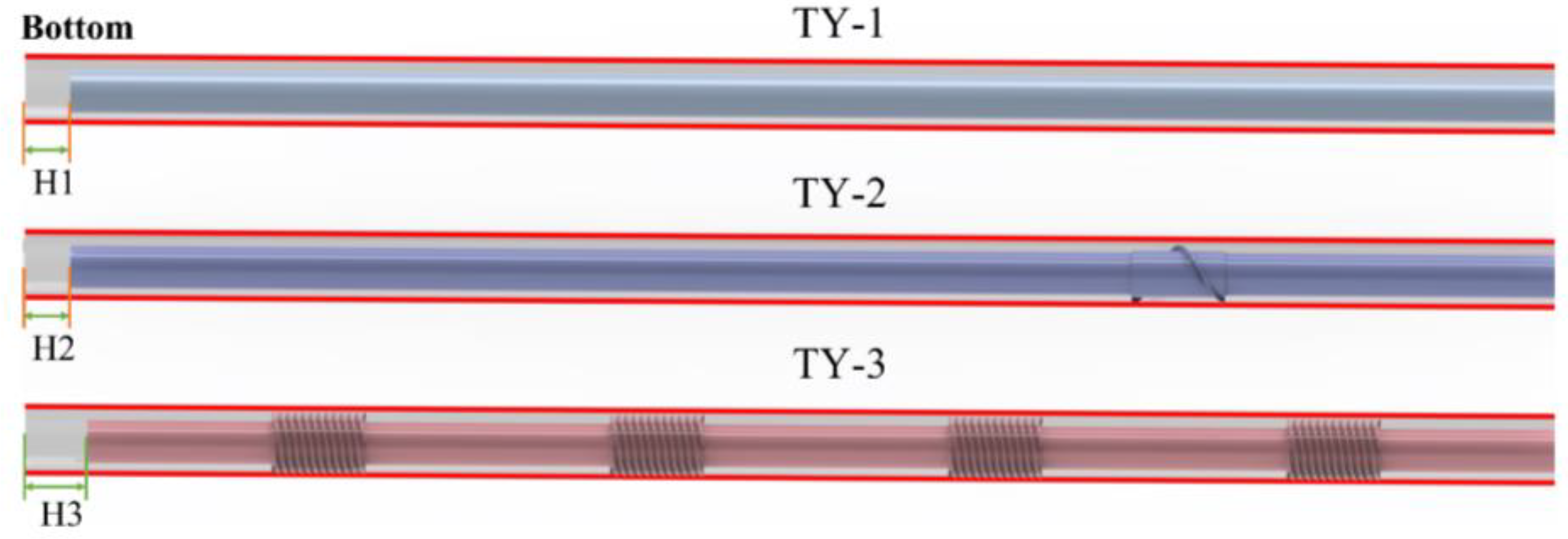
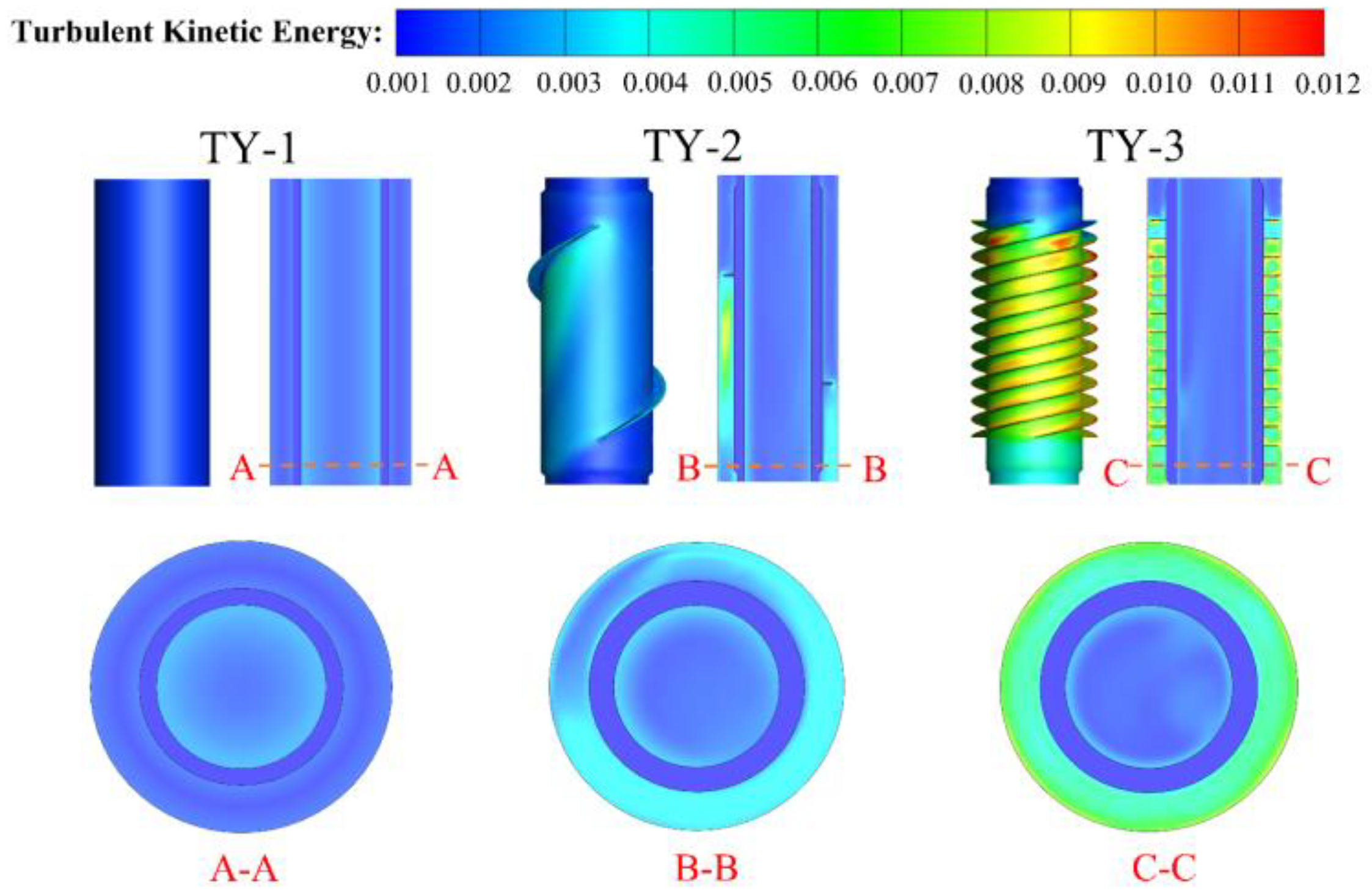
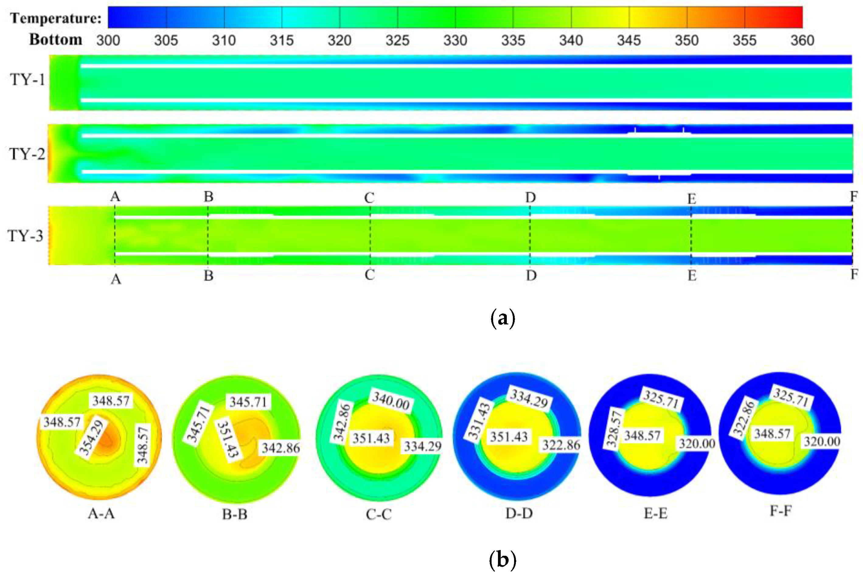
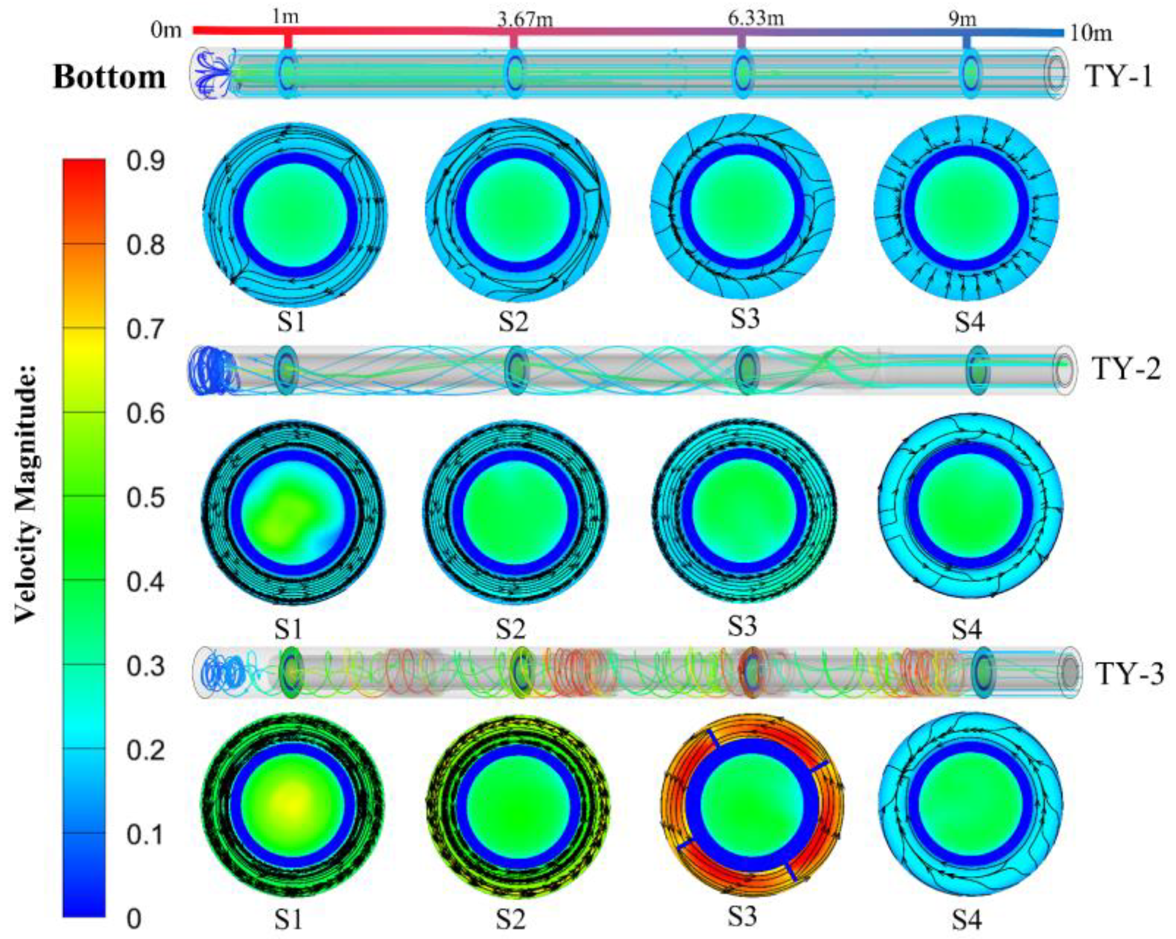
| TY-1 | the smooth pipe structure |
| TY-2 | The structure of considering the single-factor optimization of SFCBHE |
| TY-3 | the structure obtained by considering the multifactorial coupling effect |
| I-1 | the elevated temperature of TY-3 relative to TY-1 |
| I-2 | the elevated temperature of TY-3 relative to TY-2 |
| L-1 | the enhancement rate of heat extraction power of TY-3 relative to TY-1 |
| L-2 | the enhancement rate of heat extraction power of TY-3 relative to TY-2 |
References
- Rohit, R.V.; Kiplangat, D.C.; Veena, R.; Jose, R.; Pradeepkumar, A.P.; Kumar, K.S. Tracing the evolution and charting the future of geothermal energy research and development. Renew. Sustain. Energy Rev. 2023, 184, 113531. [Google Scholar]
- Dincer, I.; Rosen, M.A. Exergy Analysis of Heating, Refrigerating and Air Conditioning: Methods and Applications; Elsevier: Amsterdam, The Netherlands, 2015. [Google Scholar]
- Dor, J.; Wang, G.L.; Zheng, K.Y. Study on the Development and Utilization Strategy of Geothermal Resources in China; Science Press: Beijing, China, 2017. [Google Scholar]
- Dor, J. The basic characteristics of the Yangbajing geothermal field—A typical high temperature geothermal system. Eng. Sci. 2003, 5, 42. [Google Scholar]
- Cao, R.; Dor, J.; Li, Y.; Meng, H.; Cai, Y. Occurrence characteristics, development status, and prospect of deep high-temperature geothermal resources in China. Chin. J. Eng. 2022, 44, 1623–1631. [Google Scholar] [CrossRef]
- Dai, C.; Li, J.; Shi, Y.; Zeng, L.; Lei, H. An experiment on heat extraction from a deep geothermal well using a downhole coaxial open loop design. Appl. Energy 2019, 252, 113447. [Google Scholar] [CrossRef]
- Huang, Y. Research on Heat Transfer Mechanism and Thermal Reservoir Enhancement of Deep Coaxial Borehole Heat Exchanger in Cold Region. Ph.D. Thesis, Jilin University, Jilin, China, 2021. [Google Scholar] [CrossRef]
- Holmberg, H.; Acuña, J.; Næss, E.; Sønju, O.K. Thermal evaluation of coaxial deep borehole heat exchangers. Renew. Energy 2016, 97, 65–76. [Google Scholar] [CrossRef]
- Beier, R.A.; Acuña, J.; Mogensen, P.; Palm, B. Transient heat transfer in a coaxial borehole heat exchanger. Geothermics 2014, 51, 470–482. [Google Scholar] [CrossRef]
- Ramesh, K.; Oudina, F.M.; Souayeh, B. Mathematical Modelling of Fluid Dynamics and Nanofluids; CRC Press: Boca Raton, FL, USA, 2023. [Google Scholar]
- Mebarek-Oudina, F.; Chabani, I. Review on nano-fluids applications and heat transfer enhancement techniques in different enclosures. J. Nanofluids 2022, 11, 155–168. [Google Scholar] [CrossRef]
- Bouselsal, M.; Mebarek-Oudina, F.; Biswas, N.; Ismail, A.A.I. Heat Transfer Enhancement Using Al2O3-MWCNT Hybrid-Nanofluid inside a Tube/Shell Heat Exchanger with Different Tube Shapes. Micromachines 2023, 14, 1072. [Google Scholar] [CrossRef]
- Zanchini, E.; Lazzari, S.; Priarone, A. Improving the thermal performance of coaxial borehole heat exchangers. Energy 2010, 35, 657–666. [Google Scholar] [CrossRef]
- Chen, K.; Zheng, J.; Li, J.; Shao, J.; Zhang, Q. Numerical study on the heat performance of enhanced coaxial borehole heat exchanger and double U borehole heat exchanger. Appl. Therm. Eng. 2022, 203, 117916. [Google Scholar] [CrossRef]
- Gascuel, V.; Raymond, J.; Rivard, C.; Marcil, J.S.; Comeau, F.A. Design and optimisation of deep coaxial borehole heat exchangers for cold sedimentary basins. Geothermics 2022, 105, 102504. [Google Scholar] [CrossRef]
- Jia, L.; Cui, P.; Liu, Y.; Lu, L.; Fang, Z. Analytical heat transfer model for coaxial heat exchangers based on varied heat flux with borehole depth. Appl. Therm. Eng. 2023, 218, 119317. [Google Scholar] [CrossRef]
- Abdelhafiz, M.M.; Oppelt, J.F.; Brenner, G.; Hegele, L.A., Jr. Application of a thermal transient subsurface model to a coaxial borehole heat exchanger system. Geoenergy Sci. Eng. 2023, 227, 211815. [Google Scholar] [CrossRef]
- Rajeh, T.; Al-Kbodi, B.H.; Yang, L.; Zhao, J.; Zayed, M.E. A novel oval-shaped coaxial ground heat exchanger for augmenting the performance of ground-coupled heat pumps: Transient heat transfer performance and multi-parameter optimization. J. Build. Eng. 2023, 79, 107781. [Google Scholar] [CrossRef]
- Sun, L.; Fu, B.; Wei, M.; Zhang, S. Analysis of Enhanced Heat Transfer Characteristics of Coaxial Borehole Heat Exchanger. Processes 2022, 10, 2057. [Google Scholar] [CrossRef]
- Pérez-Zárate, D.; Santoyo, E.; Acevedo-Anicasio, A.; Díaz-González, L.; García-López, C. Evaluation of artificial neural networks for the prediction of deep reservoir temperatures using the gas-phase composition of geothermal fluids. Comput. Geosci. 2019, 129, 49–68. [Google Scholar] [CrossRef]
- Tut Haklidir, F.S.; Haklidir, M. Prediction of reservoir temperatures using hydrogeochemical data, Western Anatolia geothermal systems (Turkey): A machine learning approach. Nat. Resour. Res. 2020, 29, 2333–2346. [Google Scholar] [CrossRef]
- El Jery, A.; Khudhair, A.K.; Abbas, S.Q.; Abed, A.M.; Khedher, K.M. Numerical simulation and artificial neural network prediction of hydrodynamic and heat transfer in a geothermal heat exchanger to obtain the optimal diameter of tubes with the lowest entropy using water and Al2O3/water nanofluid. Geothermics 2023, 107, 102605. [Google Scholar] [CrossRef]
- Tan, Y.; Guo, L.; Gao, H.; Zhang, L. Deep coupled joint distribution adaptation network: A method for intelligent fault diagnosis between artificial and real damages. IEEE Trans. Instrum. Meas. 2020, 70, 3507212. [Google Scholar] [CrossRef]
- Zhong, K.; Zhou, G.; Deng, W.; Zhou, Y.; Luo, Q. MOMPA: Multi-objective marine predator algorithm. Comput. Methods Appl. Mech. Eng. 2021, 385, 114029. [Google Scholar] [CrossRef]
- Ramezani, M.; Bahmanyar, D.; Razmjooy, N. A new improved model of marine predator algorithm for optimisation problems. Arab. J. Sci. Eng. 2021, 46, 8803–8826. [Google Scholar] [CrossRef]
- Zhao, S.; Wu, Y.; Tan, S.; Wu, J.; Cui, Z.; Wang, Y.G. QQLMPA: A quasi-opposition learning and Q-learning based marine predators algorithm. Expert Syst. Appl. 2023, 213, 119246. [Google Scholar] [CrossRef]
- Sun, L.; Fu, B.; Wei, M.; Zhang, S. New Coaxial Borehole Heat Exchanger Strengthens Heat Transfer Research. Chin. Hydraul. Pneum. 2023, 47, 164–173. [Google Scholar]
- Nakhchi, M.E.; Esfahani, J.A. Numerical investigation of heat transfer enhancement inside heat exchanger tubes fitted with perforated hollow cylinders. Int. J. Therm. Sci. 2020, 147, 106153. [Google Scholar] [CrossRef]
- Caulk, R.A.; Tomac, I. Reuse of abandoned oil and gas wells for geothermal energy production. Renew. Energy 2017, 112, 388–397. [Google Scholar] [CrossRef]
- Xing, L.; Spitler, J.D. Prediction of undisturbed ground temperature using analytical and numerical modeling. Part I: Model development and experimental validation. Sci. Technol. Built Environ. 2016, 23, 787–808. [Google Scholar] [CrossRef]
- Webb, R.L. Perform ance evaluation criteria for use of enhanced heat transfer surfacesin heat exchanger design. Int. J. Heat Mass Transf. 1981, 24, 715–726. [Google Scholar] [CrossRef]
- Mei, R. An approximate expression for the shear lift force on a spherical particle at finite Reynolds number. Int. J. Multiph. Flow 1992, 18, 145–147. [Google Scholar] [CrossRef]
- Gnielinski, V. New equations for heat and mass transfer in turbulent pipe and channel flow. Int. Chem. Eng. 1976, 16, 359–368. [Google Scholar]
- Petukhov, B.S. Heat transfer and friction in turbulent pipe flow with variable physical properties. Adv. Heat Transf. 1970, 6, 503–564. [Google Scholar]
- Garcia, A.; Vicente, P.G.; Viedma, A. Experimental study of heat transfer enhancement with wire coil inserts in laminar-transition-turbulent regimes at different Prandtl numbers. Int. J. Heat Mass Transf. 2005, 48, 4640–4651. [Google Scholar] [CrossRef]
- Liu, Y.; Zhang, Y.; Pei, C.; Wang, Z.; Zhang, W. Evaluation on heat transfer performance of horizontal liquid-solid circulating fluidised bed heat exchanger. Chem. Ind. Eng. Prog. 2016, 35, 3421–3425. [Google Scholar]
- Faramarzi, A.; Heidarinejad, M.; Mirjalili, S.; Gandomi, A.H. Marine Predators Algorithm: A nature-inspired metaheuristic. Expert Syst. Appl. 2020, 152, 113377. [Google Scholar] [CrossRef]
- Hassan, M.H.; Yousri, D.; Kamel, S.; Rahmann, C. A modified marine predators algorithm for solving single-and multi-objective combined economic emission dispatch problems. Comput. Ind. Eng. 2021, 164, 107906. [Google Scholar] [CrossRef]
- Bartumeus, F.; Catalan, J.; Fulco, U.L.; Lyra, M.L.; Viswanathan, G.M. Optimising the encounter rate in biological interactions: Lévy versus Brownian strategies. Phys. Rev. Lett. 2002, 88, 097901. [Google Scholar] [CrossRef] [PubMed]
- Filmalter, J.D.; Dagorn, L.; Cowley, P.D.; Taquet, M. First descriptions of the behavior of silky sharks, Carcharhinus falciformis, around drifting fish aggregating devices in the Indian Ocean. Bull. Mar. Sci. 2011, 87, 325–337. [Google Scholar] [CrossRef]
- Mohammed, H.A.; Abbas, A.K.; Sherif, J.M. Influence of geometrical parameters and forced convective heat transfer in transversely corrugated circular tubes. Int. Commun. Heat Mass Transf. 2013, 44, 116–126. [Google Scholar] [CrossRef]
- Ran, Y.; Bu, X. Influence analysis of insulation on performance of single well geothermal heating system. CIESC J. 2019, 70, 4191–4198. [Google Scholar]


| Type | Parameter | Symbol | Initial Value | Ranges |
|---|---|---|---|---|
| Fixed parameters | DOTVG | L1 | 2850 mm | — |
| TL | L | 10,000 mm | — | |
| OTD | D1 | 210 mm | — | |
| ITI | D2 | 100 mm | — | |
| TVGD | D3 | 130 mm | — | |
| Optimized parameters | fin height | HC | 15 mm | 5~20 mm |
| pitch | P | 300 mm | 100~400 mm | |
| Number of fins | F | 1 | 1~4 | |
| Number of TVG | G | 1 | 1~4 | |
| TDIT | H | 200 mm | 100~700 mm |
| Parameter | Symbol | Water | Outlet Tube | Inlet Tube | Unit |
|---|---|---|---|---|---|
| Density | Ρ | 998.2 | 7850 | 962 | kg·m−3 |
| Specific heat capacity | cρ | 4182 | 502.48 | 2630 | J·(kg·K)−1 |
| Thermal conductivity | k | 0.6 | 44.19 | 0.02 | W·(m·K) |
| Viscosity | Μ | 0.001003 | — | — | kg·(m·s)−1 |
| Levels | Experimental Factors | PEC | ||||
|---|---|---|---|---|---|---|
| Hc (mm) | P (mm) | F (N/A) | G (N/A) | H (mm) | ||
| 1 | 5 | 100 | 1 | 1 | 100 | 1.036 |
| 2 | 5 | 200 | 2 | 2 | 300 | 1.038 |
| 3 | 5 | 300 | 3 | 3 | 500 | 1.035 |
| 4 | 5 | 400 | 4 | 4 | 700 | 1.012 |
| 5 | 10 | 100 | 2 | 3 | 700 | 1.119 |
| 6 | 10 | 200 | 1 | 4 | 500 | 1.102 |
| 7 | 10 | 300 | 4 | 1 | 300 | 1.042 |
| 8 | 10 | 400 | 3 | 2 | 100 | 1.075 |
| 9 | 15 | 100 | 3 | 4 | 300 | 1.275 |
| 10 | 15 | 200 | 4 | 3 | 100 | 1.224 |
| 11 | 15 | 300 | 1 | 2 | 700 | 1.073 |
| 12 | 15 | 400 | 2 | 1 | 500 | 1.049 |
| 13 | 20 | 100 | 4 | 2 | 500 | 1.314 |
| 14 | 20 | 200 | 3 | 1 | 700 | 1.138 |
| 15 | 20 | 300 | 2 | 4 | 100 | 1.250 |
| 16 | 20 | 400 | 1 | 3 | 300 | 1.155 |
| Parameter | Symbol | Value |
|---|---|---|
| GA | Population size | 10 |
| Number of iterations | 30 | |
| Crossover probability | 0.8 | |
| Probability of variation | 0.2 | |
| BPNN | Input Variables | 5 |
| Number of hidden layers | 1 | |
| Number of neurons in the hidden layer | 10 | |
| Maximum number of iterations | 1000 | |
| Learning rate | 0.01 | |
| Precision | 0.0001 |
| Parameter | Symbol | Value |
|---|---|---|
| Discount factor | 0.5 | |
| Learning rates | 0.01 | |
| FADs | N/A | 0.2 |
| Step size factors | P | 0.5 |
| Number of iterations | I | 500 |
| Search agent | N/A | 25 |
| Discount factor | 0.5 |
| MPA | Value | GWO | Value | PSO | Value |
|---|---|---|---|---|---|
| Parameter | Parameter | Parameter | |||
| FADs | 0.2 | Dimension | 5 | Population size | 50 |
| Step size factors | 0.5 | Number of Iterations | 500 | Dimension | 5 |
| Number of Iterations | 500 | Search Agent | 25 | Acceleration constant | 0.2 |
| FADs | 0.2 | Dimension | 5 | Population size | 50 |
| Type | Hc | P | F | G | H | PEC | Ibest |
|---|---|---|---|---|---|---|---|
| QLMPA | 20 | 100 | 4 | 3.45 | 408.5 | 1.423 | 45 |
| MPA | 20 | 100 | 4 | 3.45 | 408.5 | 1.423 | 68 |
| GWO | 20 | 100 | 4 | 3.45 | 408.5 | 1.423 | 86 |
| PSO | 19.5 | 100 | 3.83 | 4 | 294.9 | 1.419 | 66 |
| Type | Hc | P | F | G | H | PEC |
|---|---|---|---|---|---|---|
| Unit | mm | mm | pieces | pieces | mm | N/A |
| TY-1 | – | – | – | – | 300 | 1.04 |
| TY-2 | 15 | 300 | 1 | 1 | 300 | 1.10 |
| TY-3 | 20 | 100 | 4 | 4 | 408.5 | 1.36 |
Disclaimer/Publisher’s Note: The statements, opinions and data contained in all publications are solely those of the individual author(s) and contributor(s) and not of MDPI and/or the editor(s). MDPI and/or the editor(s) disclaim responsibility for any injury to people or property resulting from any ideas, methods, instructions or products referred to in the content. |
© 2023 by the authors. Licensee MDPI, Basel, Switzerland. This article is an open access article distributed under the terms and conditions of the Creative Commons Attribution (CC BY) license (https://creativecommons.org/licenses/by/4.0/).
Share and Cite
Fu, B.; Guo, Z.; Yan, J.; Sun, L.; Zhang, S.; Nie, L. Research on the Heat Extraction Performance Optimization of Spiral Fin Coaxial Borehole Heat Exchanger Based on GA–BPNN–QLMPA. Processes 2023, 11, 2989. https://doi.org/10.3390/pr11102989
Fu B, Guo Z, Yan J, Sun L, Zhang S, Nie L. Research on the Heat Extraction Performance Optimization of Spiral Fin Coaxial Borehole Heat Exchanger Based on GA–BPNN–QLMPA. Processes. 2023; 11(10):2989. https://doi.org/10.3390/pr11102989
Chicago/Turabian StyleFu, Biwei, Zhiyuan Guo, Jia Yan, Lin Sun, Si Zhang, and Ling Nie. 2023. "Research on the Heat Extraction Performance Optimization of Spiral Fin Coaxial Borehole Heat Exchanger Based on GA–BPNN–QLMPA" Processes 11, no. 10: 2989. https://doi.org/10.3390/pr11102989
APA StyleFu, B., Guo, Z., Yan, J., Sun, L., Zhang, S., & Nie, L. (2023). Research on the Heat Extraction Performance Optimization of Spiral Fin Coaxial Borehole Heat Exchanger Based on GA–BPNN–QLMPA. Processes, 11(10), 2989. https://doi.org/10.3390/pr11102989