Article

Wear Prediction of Tool Based on Modal Decomposition and MCNN-BiLSTM

1
School of Automation and Electrical Engineering, Shenyang Ligong University, Shenyang 110159, China
2
Liaoning Key Laboratory of Information Physics Fusion and Intelligent Manufacturing for CNC Machine, Shenyang Institute of Technology, Fushun 113122, China
3
School of Automation, Shenyang Institute of Engineering, Shenyang 110136, China
4
Department of Computer Science, University of Bradford, Bradford BD71DP, UK
*
Author to whom correspondence should be addressed.
Processes 2023, 11(10), 2988; https://doi.org/10.3390/pr11102988
Submission received: 31 August 2023 / Revised: 3 October 2023 / Accepted: 7 October 2023 / Published: 16 October 2023

Abstract

:
Metal cutting is a complex process with strong randomness and nonlinear characteristics in its dynamic behavior, while tool wear or fractures will have an immediate impact on the product surface quality and machining precision. A combined prediction method comprising modal decomposition, multi-channel input, a multi-scale Convolutional neural network (CNN), and a bidirectional long-short term memory network (BiLSTM) is presented to monitor tool condition and to predict tool-wear value in real time. This method considers both digital signal features and prediction network model problems. First, we perform correlation analysis on the gathered sensor signals using Pearson and Spearman techniques to efficiently reduce the amount of input signals. Second, we use Complete ensemble empirical mode decomposition with adaptive noise (CEEMDAN) to enhance the local characteristics of the signal, then boost the neural network’s identification accuracy. In addition, the deconstructed signal is converted into a multi-channel input matrix, from which multi-scale spatial characteristics and two-way temporal features are recovered using multi-scale CNN and BiLSTM, respectively. Finally, this strategy is adopted in simulation verification using real PHM data. The wear prediction experimental results show that, in the developed model, C1, C4, and C6 have good prediction performance, with RMSE of 8.2968, 12.8521, 7.6667, and MAE of 6.7914, 9.9263, and 5.9884, respectively, significantly lower than SVR, B-BiLSTM, and 2DCNN models.

1. Introduction

Tool wear and fracture can directly impair surface quality and machining precision throughout the manufacturing process. In severe circumstances, they can potentially lead to machine tool accidents. Traditional machining procedures rely on manual experience to identify when to change tools, such as running duration, cutting sound, and tool surface color, whereas subjective judgment approaches have drawbacks [1]. According to the results in [2], tool breakage accounts for 7% of machine downtime. Tool monitoring systems are expected to be a necessary and vital component of manufacturing systems with the increasing use of flexible manufacturing systems, intelligent manufacturing systems and computer-integrated manufacturing systems [3].

1.1. Literature Review

Three types of widely used prediction models are empirical, mechanism analysis-based, and data-driven [4]. Most academics currently use data-driven life monitoring techniques, since empirical models and mechanism analysis are not universally applicable, and building complicated models is challenging. Machine learning models and degradation-based models are the two primary categories of data-driven models. Cutting tool degradation models have been broken down by researchers into approaches based on gamma processes [5], Markov processes, and Wiener processes [6]. The accuracy of tool life prediction will be impacted by the choice of degradation models, since different types of cutting tools have distinct degradation models. By continually developing the corresponding relationship between the real-time equipment monitoring data (or extracted characteristics) and the present wear value, tool wear prediction is accomplished using machine learning prediction methods. Machine learning-based approaches can solve the issue of incorrect or ambiguous tool degradation model selection; meanwhile, the input of the model is not constrained to a particular type of monitoring data.
The cutting force, vibration, and acoustic emission signals are the most commonly used in tool monitoring studies [7,8,9,10]. The cutting force signal rises when the tool is passivated [11,12]. Acoustic emission signals are created during the machining process as a result of the cutting tool’s quick interaction with the treated material. Acoustic emission sensors have also been widely employed due to their high sensitivity, excellent anti-interference capabilities, and ease of installation [13,14]. Because friction between the cutting tool and the workpiece can modify the dynamic component of the cutting force, vibration during the cutting process includes vital information regarding the cutting tool’s wear condition [15].
The traditional machine learning approaches for predicting tool wear status primarily use multi-layer perceptron (MLP) [16,17], radial basis function (RBF) [18,19], extreme learning machines (ELMS) [20,21], and support vector machines (SVM) [22,23]. However, as sensor technology is rapidly developed in the big data, cloud computing age, industrial systems can now receive an increasing amount of monitoring data. It is challenging to automatically grasp and evaluate large amounts of monitoring data using traditional neural network techniques. With its potent feature extraction capabilities, deep learning, a new technique derived from neural networks, offers a new prediction strategy for training huge amounts of data. Convolutional neural networks (CNN) [24,25] and recurrent neural networks (RNN) [26,27] are the two primary types of prediction algorithms in use today. Additionally, deep learning prediction has been effectively used in several technical disciplines, including the prediction of natural gas and oil extraction [28,29], industrial system faults [30,31], and others.
A brief synopsis of the literature under study is given in Table 1. Specific material physical models, neural networks, support vector machines, deep learning models, and other machine learning techniques have demonstrated great performance in the research of tool wear prediction while processing sizable volumes of nonlinear data. To disclose the intrinsic properties of the sensor signal in the cutting process and increase prediction accuracy, researchers employ methods including attention mechanisms, principal component analysis, and multi-channel fusion. Monitoring the wear status of cutting tools by collecting sensor signals, metal cutting is still a challenging process with highly unpredictable and nonlinear dynamic behavior. It is required to separate out characteristics from a vast number of non-stationary data gathered by sensors to anticipate tool wear effectively and dependably. In addition to information on tool wear, sensor signals also contain a variety of interference signals, such as noise. In order to anticipate the wear state, it is therefore important to analyze the original signal suitably and extract signal elements linked to the tool state along with a better neural network prediction model [32].

1.2. Research Gaps and Contributions

Following the introduction above, the main contributions of this study are summarized as follows:
(1) To reduce the signal amount of the input deep learning model, amplify local signal features, and increase the identification accuracy of the prediction model for tool wear status, correlation analysis and signal modal decomposition algorithms are introduced in the signal processing of the collected tool wear sensor.
(2) To increase the predictability of tool wear status, the tool wear prediction model employs a combination prediction technique, paired with residual structure, employing MCNN to extract multi-scale spatial features and BiLSTM to extract bidirectional temporal features.
The remainder of this paper is organized as follows. The monitoring framework and data processing algorithm design for tool wear status in this study are covered in the second part; Section 3 demonstrates the design of the Deep Learning Network; Section 4, Experimental validation and analysis using real data, compares and analyzes the experimental results of the proposed technique with Support Vector Regression (SVR), Gated Recurrent Unit Neural Network (GRU), Bayesian optimization LSTM and BiLSTM, One-Dimensional Convolutional Neural Network (1DCNN) and LSTM combination prediction algorithm and two-dimensional Convolutional Neural Network (2DCNN).

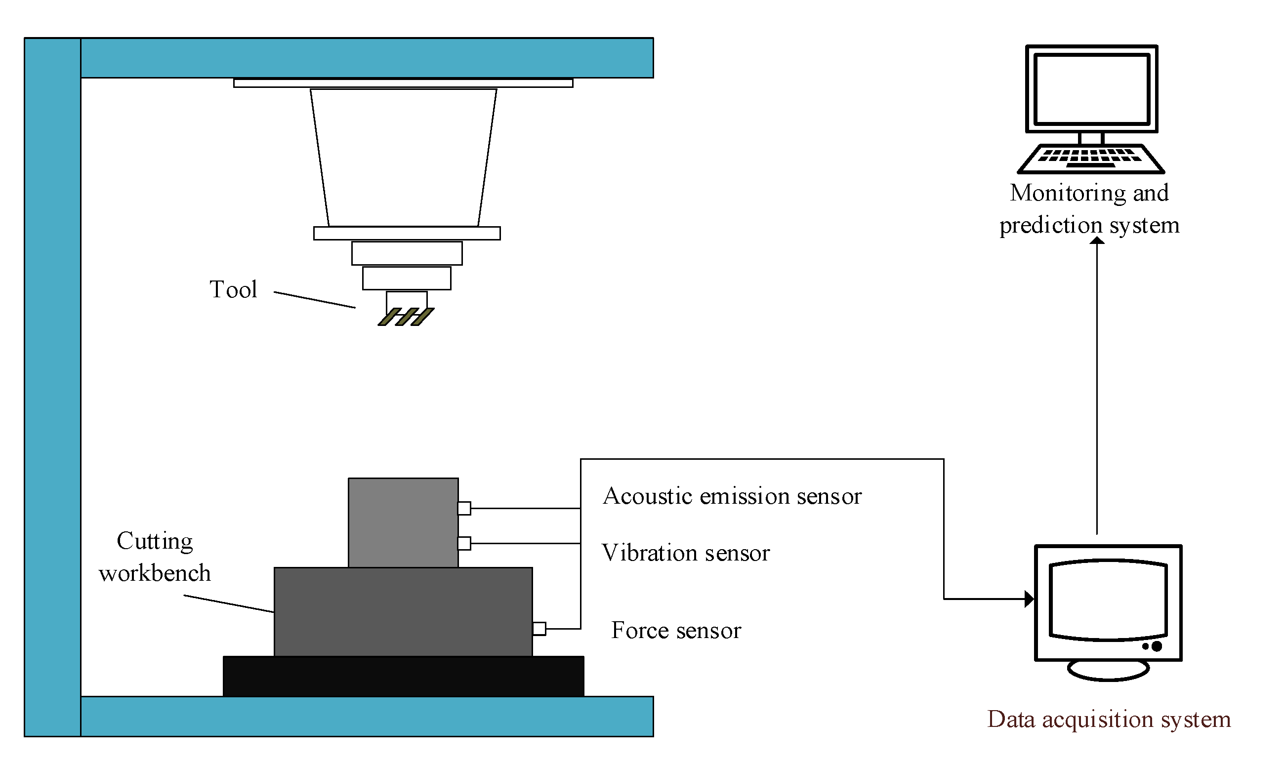
2. Problem Description

The quality of feature extraction limits the accuracy of the “feature extraction + machine learning model” in its conventional sense. There may be some information loss when converting signals to frequency or time-frequency domains for analysis. In addition to being adept at watching and finding, researchers also need to have a certain set of abilities and expertise in order to extract characteristics that are highly associated with tool wear state [42]. Additionally, the retrieved characteristics have poor universality and interpretability, and it is possible that more delicate traits were left out. For the self-coding network, if the number of network layers is too great, the model may not succeed owing to the lack of global optimization of the entire model. The model built by a convolutional neural network relies on the extraction of high-dimensional features by a convolution operation, but a small number of convolution operations cannot accurately predict the tool wear. The method proposed in this article aims to accurately predict the wear value changes of cutting tools during machining by collecting multidimensional sensor signals, as shown in Figure 1. The accuracy of prediction methods is crucial for the operation and efficiency of enterprise production and machine tool processing.

3. Predicting Tool Wear Based on MCNN BiLSTM

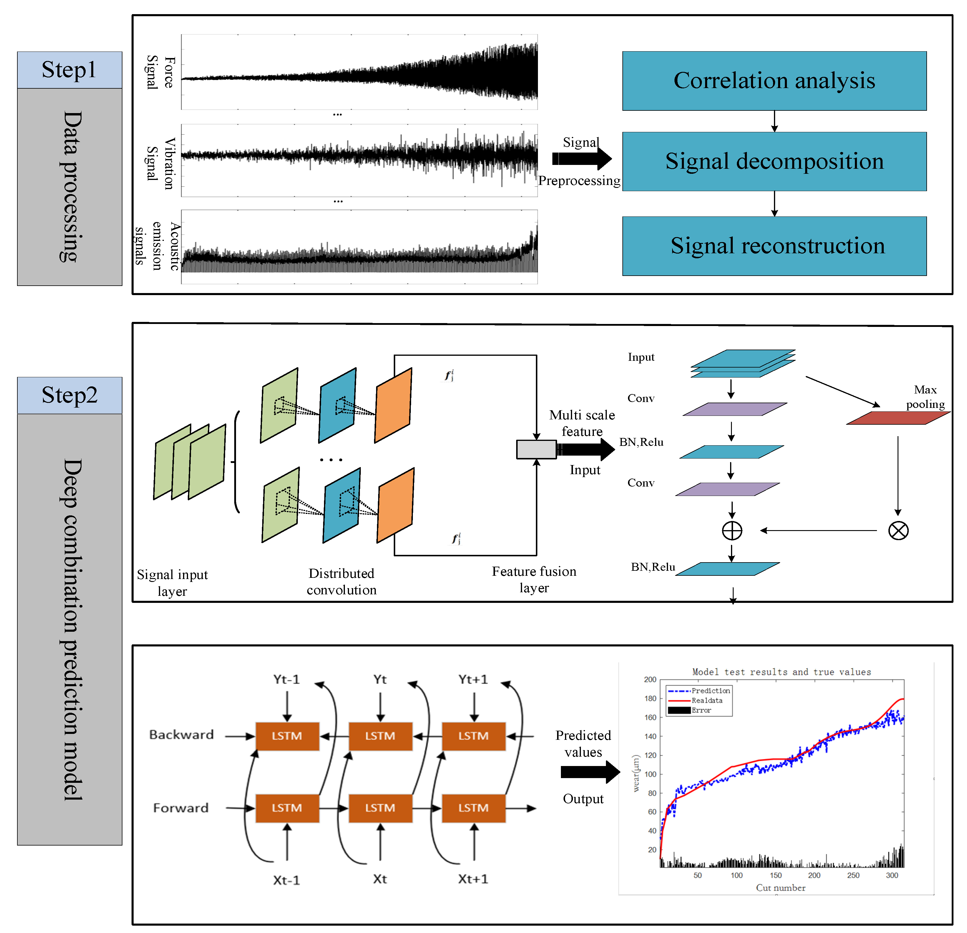
3.1. Tool Wear Prediction Framework

Force, vibration, and acoustic emission sensors are employed during the cutting process to gather indications pertaining to tool wear. The sensor installation is displayed. A three-dimensional force measurement device is installed between the workstation and the object to be machined in order to gauge the cutting forces in the X, Y, and Z axes; a piezoelectric accelerometer is installed on the workpiece to track the X, Y, and Z vibration signals as the tool is being processed; and for the purpose of measuring the high-frequency stress waves produced during the cutting process, an acoustic emission sensor is mounted on the workpiece. Consequently, the data’s final dimension is seven. A structural charge amplifier boosts the sensor signal, which is then recorded by a data gathering system. A microscope is used to assess the tool’s back face offline wear state after the tool’s end face has been milled. A deep learning network is used to process and import the signal for training, creating an entire tool mode monitoring and prediction system. Data processing is used to enhance signal features [43], deep learning networks are used to process and import signals for training, and the entire tool pattern monitoring and prediction system is created, as shown in Figure 2.

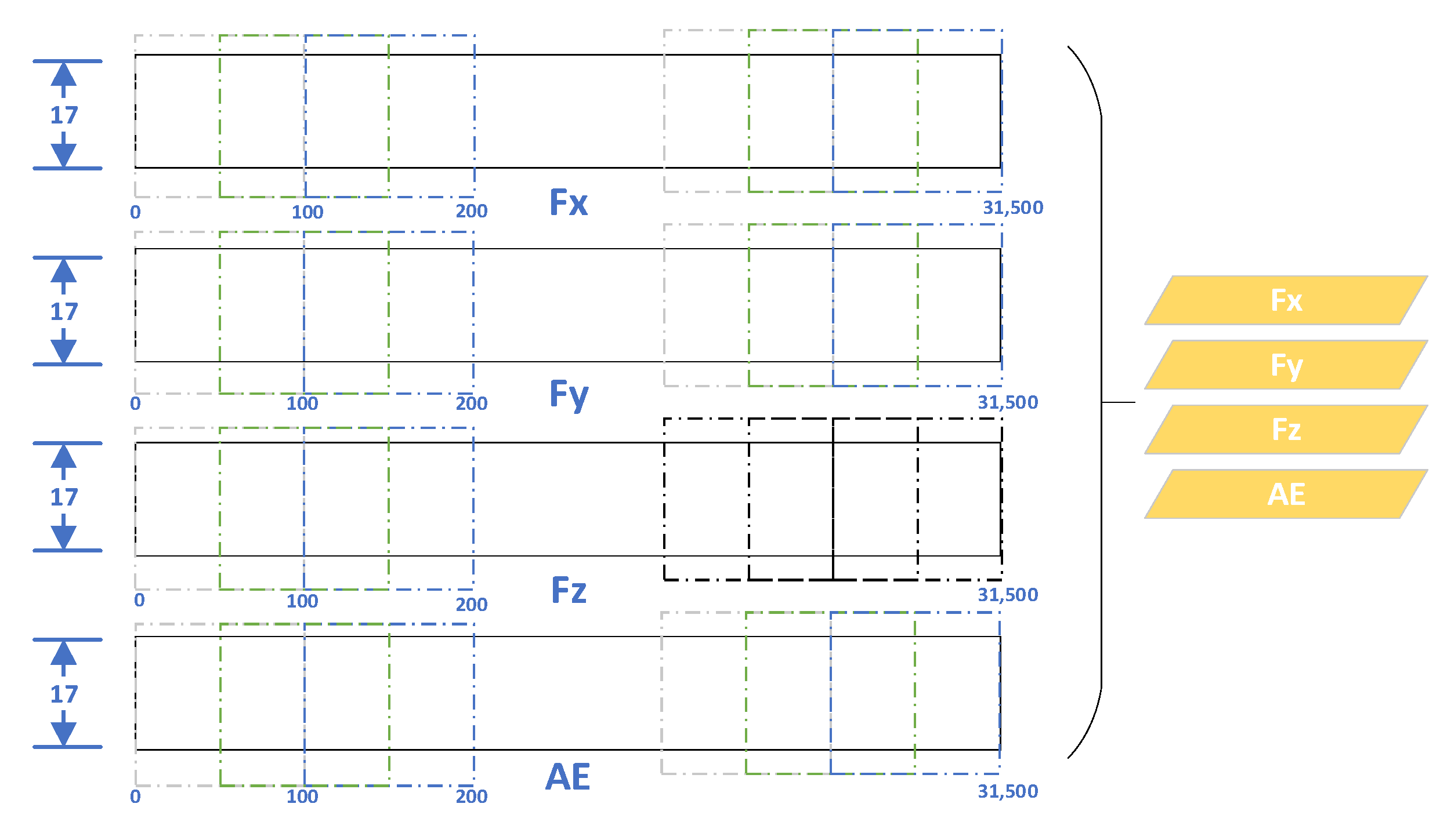
3.2. Data Processing

3.2.1. Multivariate Correlation Analysis

A prominent technique for data correlation analysis is Pearson and Spearman correlation analysis [44]. It may be applied to determine the linear correlation, or relationship between two variables. The related formulae are shown by Equations (1) and (2),
P x y = i = 1 n x i x y i y     i = 1 n x i x 2 i = 1 n y i y 2
S x y = 1 6 i = 1 n R x i R y i 2   n n 2 1
where   P x y , S x y are Pearson correlation coefficients and Spearman correlation coefficients, respectively; x i and y i are the signals for each cutting, respectively; x and y are the mean values of two n-dimensional signals, respectively; and R x i   and R y i are the sorting in their respective signals.

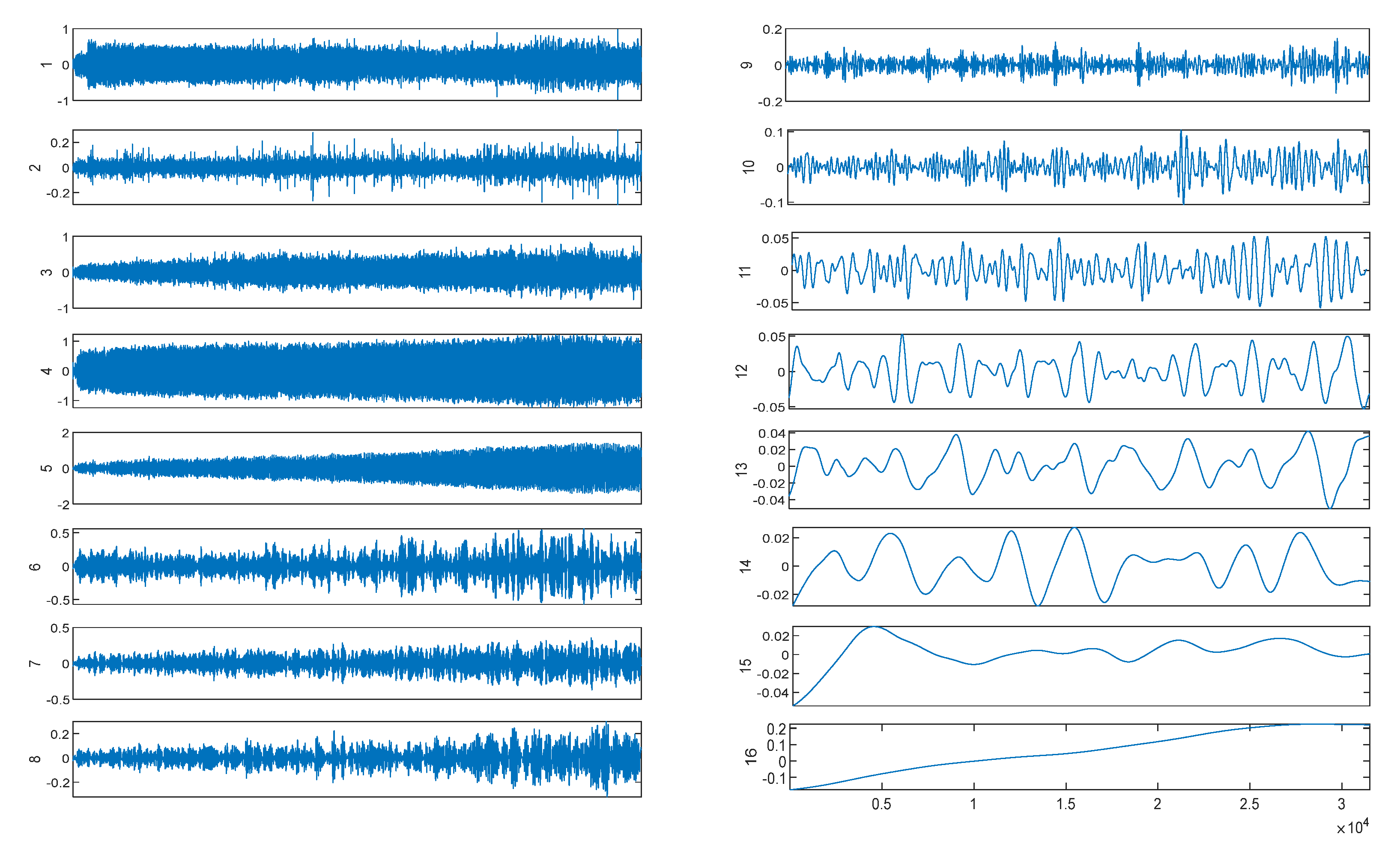
3.2.2. Empirical Mode Decomposition

Complete ensemble empirical mode decomposition with adaptive noise (CEEMDAN) is an improved empirical mode decomposition (EMD) method that can better handle nonlinear and non-stationary signals [45]. CEEMDAN obtains multiple sets of Intrinsic Mode Function (IMF) components by randomly perturbing and decomposing the signal multiple times and averages them to obtain the final IMF component. Let E i ( . ) represent the ith subsequence obtained by EMD decomposition. C i ( t ) represents the ith subsequence obtained by CEEMDAN decomposition, v j represents the Gaussian white noise signal satisfying the standard normal distribution, j = 1, 2, N represents the number of additions of white noise, d represents the standard white noise table, and y ( t ) represents the signal to be decomposed. The specific steps of the CEEMDAN method are illustrated as follows [46].
(1)
Perform multiple random perturbations on the original sensor signal y ( t ) to obtain multiple sets of disturbance signals: y ( t ) + ( 1 ) q ε v j ( t ) , q = 1,2 ; EMD decomposes the new signal to obtain the first subsequence:
E ( y ( t ) + ( 1 ) q ε v j ( t ) ) = C 1 ( t ) + r j
(2)
By averaging the created N subsequences, the first subsequence of the CEEMDAN decomposition is obtained, and the residual of the first subsequence is also calculated to be removed.
C 1 ( t ) = 1 N j = 1 N C 1 j ( t ) r 1 ( t ) = y ( t ) C 1 ( t )
(3)
Add a pair of positive and negative white Gaussian noise to r 1 ( t ) to obtain a new signal. Use the new signal as the carrier for EMD decomposition to obtain the first subsequence D 1 , from which we can obtain the second subsequence of CEEMDAN decomposition and the residual after eliminating the second subsequence.
C 2 ( t ) = 1 N j = 1 N D 1 j ( t ) r 2 ( t ) = y ( t ) C 2 ( t )
(4)
Repeat the above steps until the residual signal obtained is a monotonic function and cannot be further decomposed. The original signal is reproduced as follows:
y ( t ) = k = 1 k C k ( t ) + r k ( t )
The CEEMDAN method can better handle nonlinear and non-stationary signals; by multiple random perturbations and decomposition, the pseudo-components and modal aliasing phenomena of EMD methods can be reduced; the CEEMDAN method does not require a predetermined number of components in the signal and can adaptively decompose the signal. Therefore, the CEEMDAN method has been widely applied in the field of signal processing [47].

3.3. Deep Combination Prediction Model

The MCNN-BiLSTM composite model includes a multi-scale convolution layer, batch normalization layer, activation function layer, max pooling layer, BiLSTM layer, full connection layer and dropout layer. The residual block in the input block consists of two branches: the main path and the branch path. The main path contains convolutional layers, BN layers, and ReLu activation layers, while the branch path only contains max pooling layers. According to the input tensor of the residual block, the two tensors are added through the main and branch paths to form the output of the residual block. Multiple residual blocks are stacked repeatedly using a multi-layer perceptron method. The output block uses the sample specification layer, ReLu activation layer, and fully connected layer to process the output tensor of multiple residual blocks. After passing through the tiling layer, the BiLSTM module generates the output of the entire model, where the model’s diagram is shown in Figure 3. The input of the model is filtered multi-channel signal data, with the corresponding label being the minimum wear label. Extracting features from different signals using multi-scale convolution with kernel sizes of 3 × 3, 4 × 4 and 5 × 5. The number of convolutional layers is set to 64, and the number of layers for BiLSTM is set to 128.
The multi-scale convolutional layers can be expressed as:
f j i = σ r W j i * X j i + B j i
where X j i is the input of the model; W j i is the convolution kernel for each layer of convolution; B j i is the number of offsets for each layer of convolution; and f j i feature vectors extracted for each convolutional block.
An often-used activation function is ReLu. An activation function in neural networks is used to alter neurons’ output, making them nonlinear. The output of the ReLU activation function is zero when the input is negative, while the function is equal to the input when the input is positive. ReLu’s key benefits are its simplicity, quickness, and effective performance in real-world applications. It can efficiently lessen the gradient vanishing issue, speed up neural network training, and improve the accuracy of neural network output. The ReLu activation function is expressed as follows:
σ r x = 0 , x < 0 x , x 0
The flatten layer’s primary function is to reduce multidimensional data structures to one-dimensional ones. This may provide the next fully linked layer or output layer a flattened data structure. The flatten layer is described by the expression:
f i = f l a t t e n f j i M j i
where f j i represents the feature vectors extracted from each convolutional block, and M j i represents the feature vectors after passing through the maximum pooling layer.
The expression for BiLSTM monitoring module to achieve prediction is shown in Equations (10)–(13):
h i = σ t W 1 f i + W 3 h i l
r i = σ t W 2 f i + W 5 r i + 1
Y i = σ t W 4 h i + W 6 r i
σ t x = e x e x e x + e x
where W 1 and W 3 have a weight matrix for feature vectors; W 2 and W 5 have a weight matrix that maps the forward and reverse layer calculation times to the current calculation times; and W 4 and W 6 have a weight matrix that maps the forward and reverse layer outputs to the output layers.

4. Validation and Analysis

4.1. Raw Data

4.1.1. Dataset Selection

The performance of the model was assessed in this study using the public dataset from the 2010 Monitoring Data Challenge [37]. Using the workpiece as a test object, six tungsten carbide ball end cutting tools (C1–C6) were employed for milling trials. Forward milling and dry cutting were used. The workpiece was made of stainless steel HRC52. Accurate cutting standard: feed speed of 1555 mm/min; cutting depths of 0.125 mm in the Y direction and 0.2 mm in the Z direction; spindle speed of 10,400 rpm. The KISTLER three-dimensional force measurement device, KISTLER piezoelectric accelerometer, and KISTLER acoustic emission sensor are the sensor models for gathering signals. The data acquisition card utilizes NIDAQPC1200, and the charge amplifier is a KISTLER charge amplifier.
Force, vibration, and acoustic emission sensors are utilized to gather electrical signals on tool wear while cutting, and Figure 4 shows the sensor installation position. A KISTLER three-dimensional force measurement device was installed between the workstation and the object to be machined in order to gauge the cutting forces in the X, Y, and Z axes; a KISTLER piezoelectric accelerometer was installed on the workpiece to track the X, Y, and Z vibration signals as the tool is being processed; and to track high-frequency stress waves produced during cutting, a KISTLER acoustic emission sensor was mounted on the workpiece. A KISTLER charge amplifier is used to increase the sensor’s output signal, and the NIDAQPC1200 is used to collect it at a sampling frequency of 50 kHz. The LEICAMZ12 microscope was used to assess the tool rear face’s wear state offline after completing 108 mm of end-face milling in the X direction. The data of 315 cuts of a tool were recorded.
Given that the dataset only contains wear-value labels for C1, C4, and C6, a cross-validation approach was utilized to verify the generalizability of the suggested strategy and assess the effectiveness of the suggested model while making full use of the dataset. C1 is the prediction set, for instance, if C4 and C6 are the training sets.

4.1.2. Data Filtering

To limit the amount of data input into the model in this study while minimizing the accuracy of network prediction, the relationship between the gathered seven-dimensional sensor signals and tool wear was checked mathematically and statistically. Thus, using Equations (1) and (2), the Pearson and Spearman correlation coefficients between sensor signals and tool wear values were determined. The results are presented in Table 2.
According to Table 2, the correlation between force signals and wear values has the greatest Pearson and Spearman correlation coefficients, but the connection between triaxial vibration signals and wear values is nearly zero. As a result, the next study will focus on the signals Fx, Fy, Vy, and AE.

4.1.3. Mode Decomposition

This study employs the CEEMDAN to decompose the signal into multiple sub-signals, each with a distinct frequency range, to avoid the deep learning model not completely mining the features in the signal. This makes it possible for the neural network to learn and interpret information throughout various frequency bands more effectively. In the circumstances, CEEMDAN can enhance the capacity of signals to extract local features, hence enhancing the recognition precision of neural networks. The performance of the neural network may be enhanced by feeding it the signal that CEEMDAN has decomposed in order to better extract its characteristics.
Therefore, this study first performs max–min normalization on sensor signals Fx, Fy, Fz, AE with greater correlation between wear values. At the same time, CEEMDAN is used to decompose the normalized signal. Taking the Fy signal as an example, 16 groups of decomposed subsequences are obtained, as shown in Figure 5. The decomposed subsequences of Fx, Fy, Fz and AE signals were combined with the corresponding original signals into a 100 × 17 × 4 multi-channel input matrix, as shown in Figure 6, for the feature extraction and mining timing rules of the model in this paper.

4.2. Evaluating Indicator

This research employs root mean square error (RMSE), mean absolute error (MAE) and coefficient of determination ( R 2 ), which are frequently used in workpiece life prediction, as quantitative indicators to evaluate the influence of the prediction model. A considerable mistake in the prediction findings is shown by bigger values for P m a e and P r m s e ; a greater degree of accuracy is indicated by lower values for P m a e and P r m s e .
P m a e = 1 n   k = 1 n y k p r e y k
P r m s e = 1 n k = 1 n y k p r e y k 2  
R 2 = ( y k p r e y k ) 2 ( y k y ¯ p r e ) 2
where y k is actual data, y k p r e is predicted data, y ¯ is average predicted data, and n is the number of test samples.

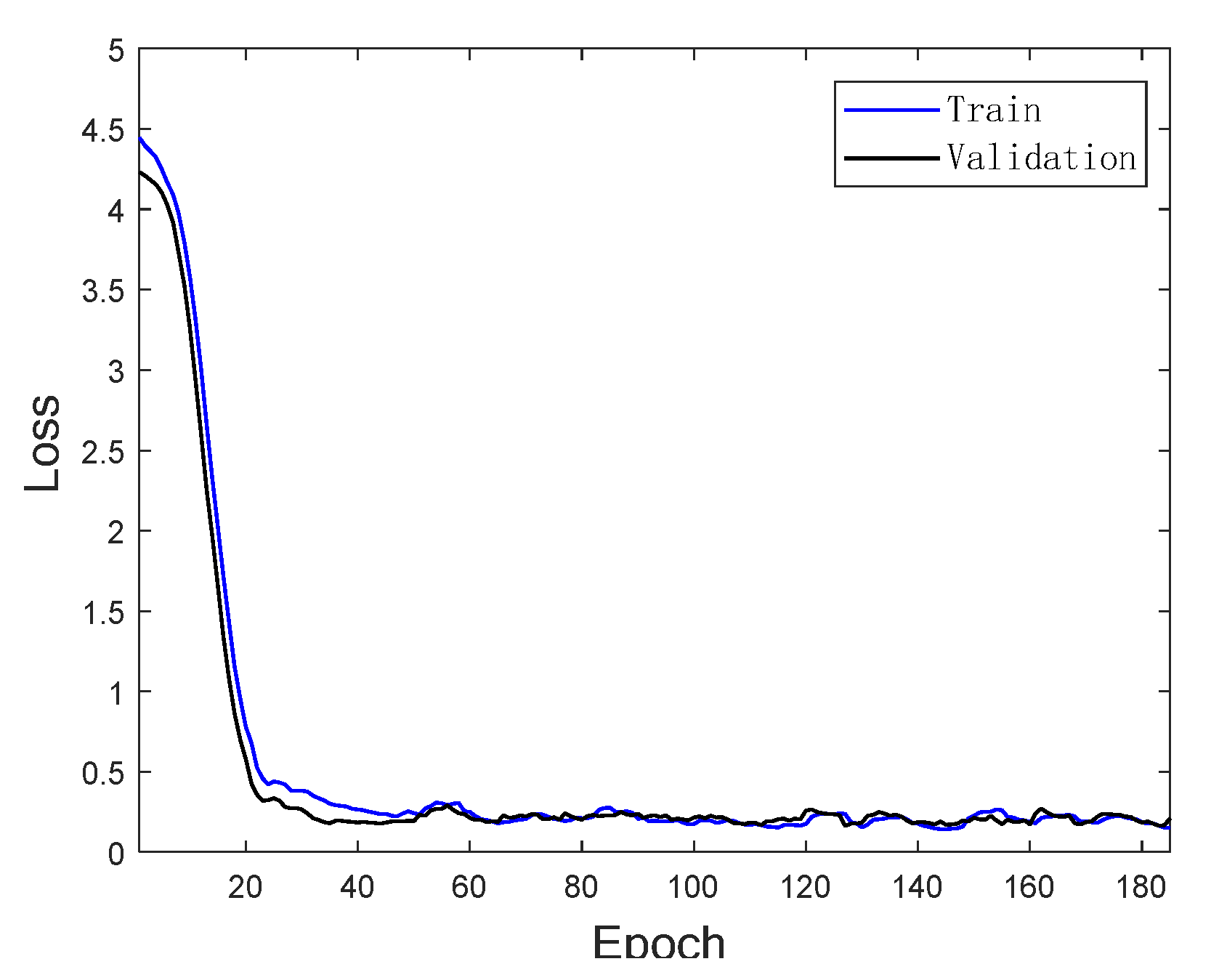
4.3. Experimental Environment

An experimental analysis was conducted on the MATLAB 2021b software platform, with hardware configuration of Intel I CoITM 7700HQ CPU and 16GB RAM, NDIVIA GTX1050, GPU; the operating system is Windows 10.
The proposed MCNN-BiLSTM prediction model includes two parts:
MCNN feature extraction and BiLSTM timing prediction. For the feature extraction part of MCNN, please note that all 2D Convs are used here, and 3D Convs are used for feature extraction, with Conv sizes of {3 × 3, 4 × 4, 5 × 5} with the 64 hidden layers. After two residual extractions, the size of Conv in the residual module is 3 × 3. The activation function of the network is ReLu; for the prediction part of BiLSTM, BiLSTM consists of a one-layer network with 128 hidden layers. The training parameters of other prediction models are shown in Table 3.

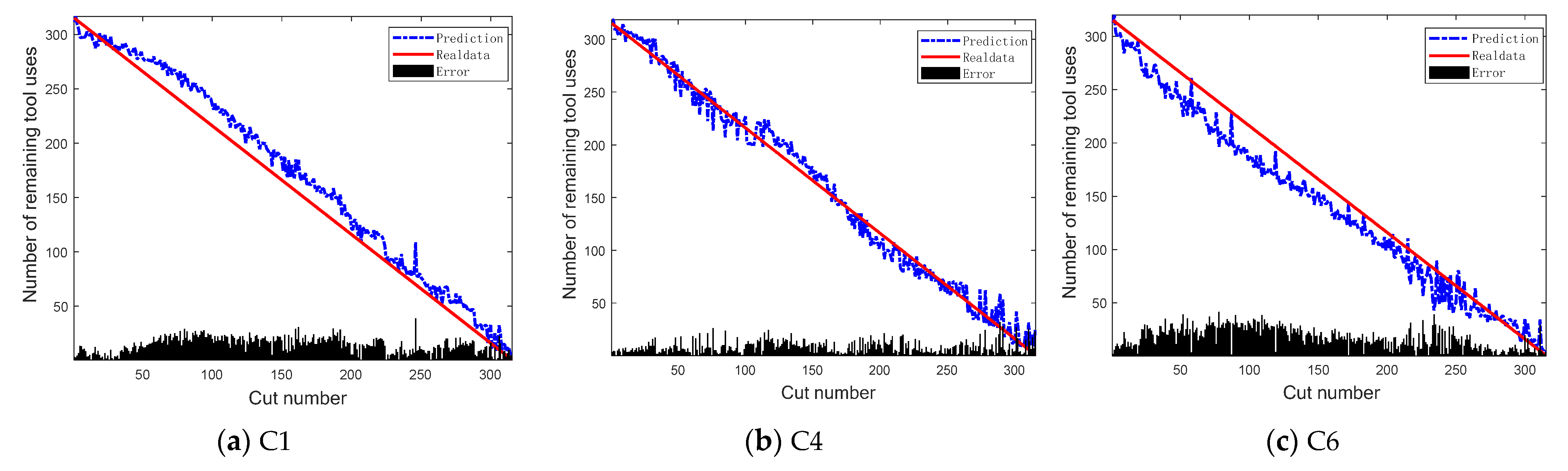
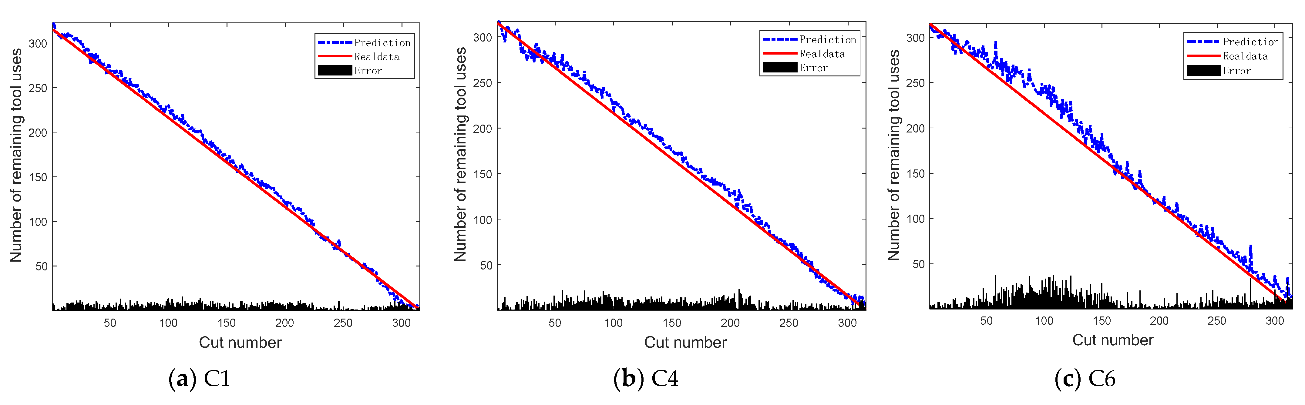
4.4. Result Analysis

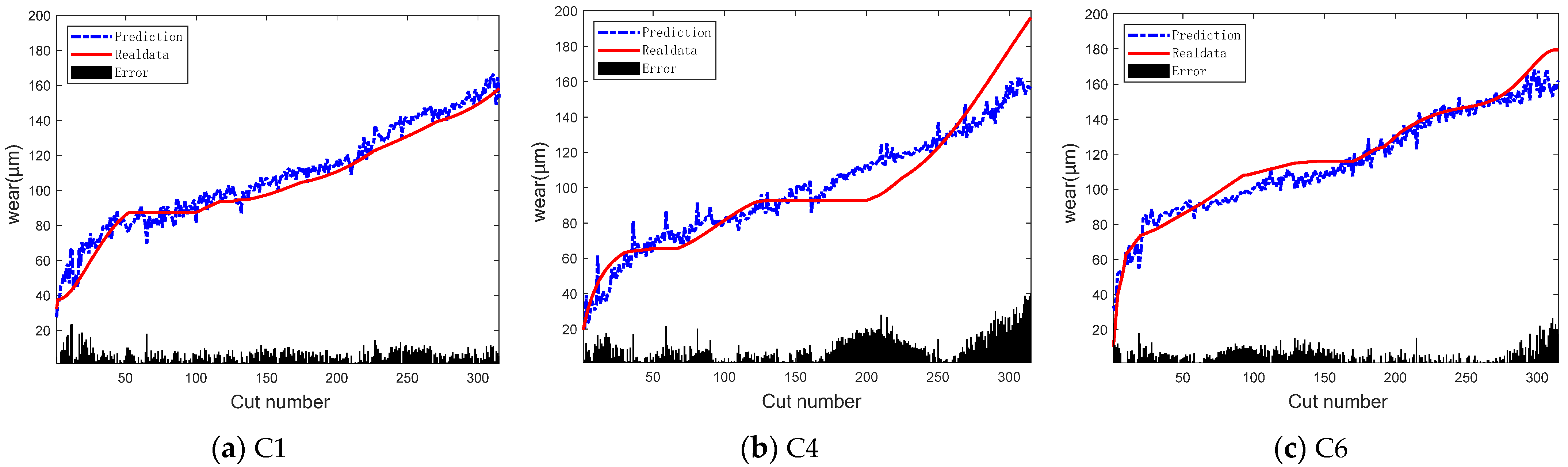
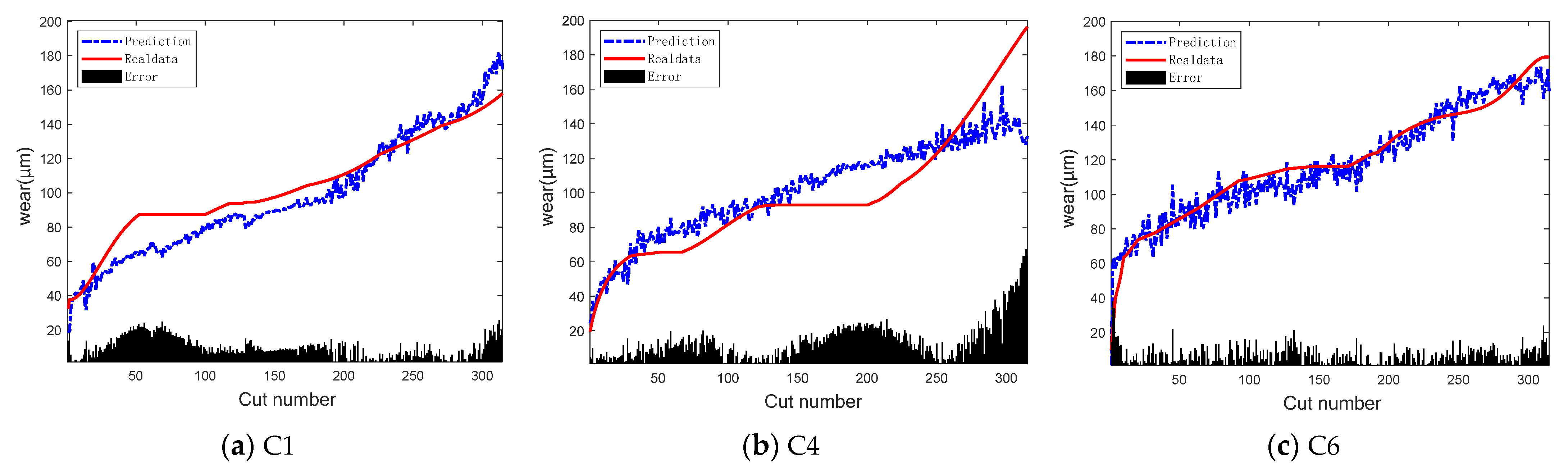
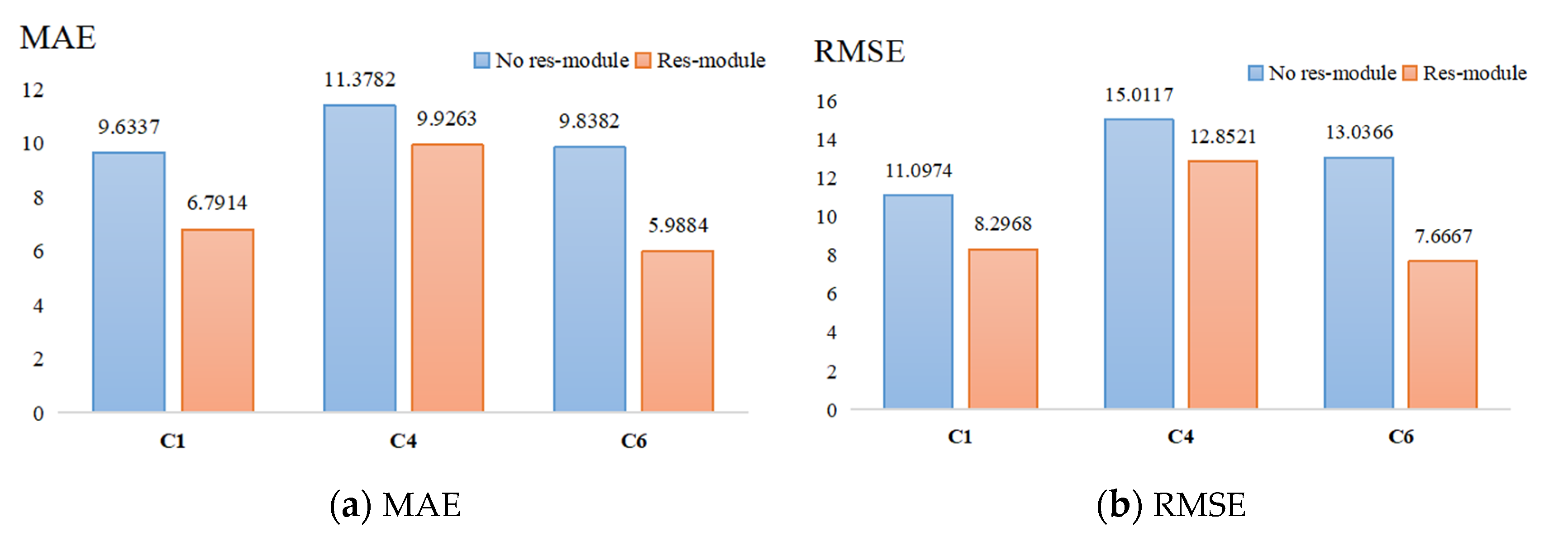
4.4.1. Module Verification

The prediction results of the proposed model under three different test tools are shown in Figure 7. In machine tool processing, milling is a slow process, and the time required for CEEMDAN’s data decomposition as well as the prediction of the model is negligible, so there is not much discussion here. It is clear that the model provides accurate tool prediction results. To better show the effectiveness of the model, the training and validation loss of the model are shown in Figure 8.
Figure 9 shows the prediction results of the original signal directly input into the proposed model, and it can be seen that the prediction effect is not as good as Figure 7.
A more thorough data comparison, examining the quantitative value of the influence of signal decomposition on model performance, may be seen in Table 4. It can be clearly seen that the RMSE and MAE of the signals predicted by tool C1 decreased by 26.54% and 29.10%, respectively, after CEEMDAN decomposition. The RMSE and MAE of C4 decreased by 29.82% and 29.29%, respectively. The RMSE and MAE of C6 decreased by 11.03% and 11.68%, respectively. In addition, the R 2 also increased, which means that using CEEMDAN results in a higher fit for both the predicted and true values.
Residual structures were introduced to the model to improve the network’s representation capabilities. As seen in Figure 10, the deep learning model with residual structures outperforms the one without the res-module. The residual network can solve the vanishing gradient problem. The gradient signal will be backpropagated numerous times in the deep neural network as the network layers expand, resulting in the gradient gradually becoming less. The residual structure allows the input signal to be directly added to the output signal, allowing the gradient of the network to be better propagated and avoiding the vanishing gradient problem. Second, the residual structure enables the network to learn the residual component, allowing it to adapt to complicated data distributions and nonlinear transformations more effectively [48]. Furthermore, employing residual structures can boost the network’s learning efficiency.

4.4.2. Comparison with Other Models

Numerous tool wear prediction techniques were chosen for quantitative comparison in order to confirm the benefits of this suggested methodology. The selected algorithms include: Support Vector Regression (SVR), Gated Recurrent Unit Neural Network (GRU), Bayesian optimization LSTM and BiLSTM, One-Dimensional Convolutional Neural Network (1DCNN), LSTM combination prediction algorithm, and Two-Dimensional Convolutional Neural Network (2DCNN).
For SVR, since SVR cannot handle sequence data, feature extraction must be carried out first. It is necessary to extract 11 characteristics from seven channel data in the time domain, including mean, standard deviation, skewness, kurtosis, pulse factor, peak factor, shape factor, marginal factor, peak-to-peak value, root mean square, and energy. The frequency domain is used to extract four characteristics, including the sk mean, sk standard deviation, and sk kurtosis, giving the seven-dimensional signal a total of 105-dimensional time-frequency features. A 105 × 1 matrix was used to represent each trimmed feature and was entered into the ensuing regression model. The optimal regularization parameters of the SVR model are selected from {0.001, 0.01, 0.1, 1,10}, and the kernel uses the Gaussian basis function (RBF) by default.
For GRU, a layer of GRU, with 64 hidden layers, regularization parameters of 1 × 10⁻², and an initial learning rate of 1 × 10⁻² is considered.
For both LSTM and BiLSTM, model parameter optimization is achieved through Bayesian parameter estimation. LSTM considers one layer, while BiLSTM considers two layers. The maximum number of Bayesian parameter estimates is 30, the regularization range is {1 × 10⁻¹⁰, 1 × 10⁻²}, and the initial learning rate range is {1 × 10⁻³, 1}.
For both 1DCNN-BiLSTM and 2DCNN, the seven channels of original data are the original input for the 1DCNN-BiLSTM prediction model, and the seven channels of signals from the CEEMDAN are the input for the 2DCNN prediction model after they have been decomposed. Table 5 displays the comparative outcomes of trials (using tool C6 as an example).
Compared to a Recurrent Neural Network (RNN), the GRU model can process sequence data better than the SVR model. SVR, on the other hand, is a variation of the Support Vector Machine (SVM) that is frequently employed for regression issues but has poor processing capability for sequential data. SVR, however, outperforms GRU when the dataset is limited, since GRU needs a bigger dataset to train on and making parameter adjustments before overfitting is a possibility. On tiny datasets, SVR performance is a little bit more consistent. In contrast to the GRU model, B-LSTM, and B-BiLSTM, Bayesian optimization establishes a Gaussian process model in the explored parameter space to estimate the unknown region of the function to be optimized, avoiding the need to search the entire parameter space, conserving computing resources, and speeding up the evaluation of the optimal solution. Compared to unidirectional LSTM, BiLSTM utilizes information from both the front and back directions, enabling a more comprehensive understanding of time series data and achieving better results.
According to Table 5, when compared to SVR, GRU, B-LSTM, and B-BiLSTM models, the suggested model in this study dramatically lowers RMSE and MAE. The comparison results demonstrate that the multi-scale data fusion model derived by this model is more sensitive to changes in tool wear status than the spatial or temporal correlation features extracted by conventional deep learning network models. The traditional machine learning approach also requires manual feature extraction and selection, which depend on the expertise and wealth of experience of professionals. In addition, feature adaptation and wear value prediction are carried out separately, and simultaneous optimization of both parts cannot be achieved. Therefore, the model prediction accuracy can easily achieve the upper limit.

4.4.3. Exploring the Expandability of Models

In the aforementioned study, cross experiments were conducted on the data sets C1, C4, and C6 to confirm the model’s efficacy and show its superiority to other models. All of the data from C1 through C6 will be used in the study to examine its generalizability. The output is the tool’s remaining use times, and the input is the matrix following CEEMDAN decomposition and rebuilding. Figure 11 continues the cross-validation using C1,C4,C6, and in Figure 12, if C1 is the validation set, then C2–C6 is the training set.
The prediction results are shown in Figure 11 and Figure 12. The MAE of C1 is 8.1137 and 5.4846, and the RMSE is 11.0498 and 7.3676, respectively. The MAE and RMSE of C4 were 8.1863 and 6.2208, 10.2017 and 8.7289, respectively. The MAE of C6 is 18.7712 and 12.0137, and the RMSE is 22.0223 and 15.9872, respectively. It can be seen that when the dataset is enlarged, the MAE predicted by the model shrinks by 30% and the RMSE by 25% on average. In practical application, with the more data obtained in the actual processing, the more abundant the data of the training model, the life degradation prediction model proposed in this paper will have better accuracy.

5. Conclusions

This study provides a combined prediction method based on modal decomposition, multi-channel input, MCNN and BiLSTM. Using the milling dataset of PHM2010 for experiments and validation, we draw the following conclusions:
(1)
The sensor signals during tool processing may better handle nonlinear and non-stationary signals after filtering and CEEMDAN, boosting local characteristics.
(2)
The developed model will predict tool wear values more accurately because it can more efficiently mine spatiotemporal properties in cutting signals.
(3)
This method’s prediction accuracy outperforms the SVR model, GRU model, B-LSTM model, B-BiLSTM model, 1DCNN-BiLSTM model, and 2DCNN model.
The research on tool wear prediction provided in this article is based on the machining circumstances of utilizing the same type of tool in the same working environment due to the dearth of rich data. Different tools and machining environments still provide difficult issues in actual machining production. This work presented an approach that will be utilized for later research to explore the usage of various cutting tools under various operating circumstances in order to further validate the precision of the forecast and the generalizability of this strategy.

Author Contributions

Conceptualization, Z.H. and Y.L.; methodology, Z.H. and Y.L.; software, Z.H.; validation, Z.H.; formal analysis, Z.H.; investigation, Z.H.; resources, Y.L.; data curation, Z.H.; writing—original draft preparation, Z.H.; writing—review and editing, Z.H., Y.L., X.P. and Q.Z.; visualization, Y.L.; supervision, Y.L.; project administration, Y.L.; funding acquisition, Y.L. All authors have read and agreed to the published version of the manuscript.

Funding

This paper is partly supported by National Science Foundation of China under Grants (62073226), Liaoning Province Natural Science Foundation (2020-KF-11-09, 2022-KF-11-1), Shen-Fu Demonstration Zone Science and Technology Plan Project (2021JH07), State Key Laboratory of Synthetical Automation for Process Industries (2023-kfkt-03).

Data Availability Statement

Not applicable.

Conflicts of Interest

The authors declare no conflict of interest.

References

  1. Yang, Y.; Guo, Y.; Huang, Z.; Chen, N.; Li, L.; Jiang, Y.; He, N. Research on the milling tool wear and life prediction by establishing an integrated predictive model. Measurement 2019, 145, 178–189. [Google Scholar] [CrossRef]
  2. Vetrichelvan, G.; Sundaram, S.; Kumaran, S.S.; Velmurugan, P. An investigation of tool wear using acoustic emission and genetic algorithm. J. Vib. Control. 2014, 21, 3061–3066. [Google Scholar] [CrossRef]
  3. Zhou, J.; Li, P.; Zhou, Y.; Wang, B.; Zang, J.; Meng, L. Toward New-Generation Intelligent Manufacturing. Engineering 2018, 4, 11–20. [Google Scholar] [CrossRef]
  4. Liao, L.; Kottig, F. Review of Hybrid Prognostics Approaches for Remaining Useful Life Prediction of Engineered Systems, and an Application to Battery Life Prediction. IEEE Trans. Reliab. 2014, 63, 191–207. [Google Scholar] [CrossRef]
  5. van Noortwijk, J. A survey of the application of gamma processes in maintenance. Reliab. Eng. Syst. Saf. 2009, 94, 2–21. [Google Scholar] [CrossRef]
  6. Zhang, Z.; Si, X.; Hu, C.; Lei, Y. Degradation Data Analysis and Remaining Useful Life Estimation: A Review on Wiener-Process-Based Methods. Eur. J. Oper. Res. 2018, 271, 775–796. [Google Scholar] [CrossRef]
  7. Toubhans, B.; Fromentin, G.; Viprey, F.; Karaouni, H.; Dorlin, T. Machinability of inconel 718 during turning: Cutting force model considering tool wear, influence on surface integrity. J. Am. Acad. Dermatol. 2020, 285, 116809. [Google Scholar] [CrossRef]
  8. Huang, Z.; Zhu, J.; Lei, J.; Li, X.; Tian, F. Tool wear predicting based on multi-domain feature fusion by deep convolutional neural network in milling operations. J. Intell. Manuf. 2020, 31, 953–966. [Google Scholar] [CrossRef]
  9. Feng, K.; Borghesani, P.; Smith, W.A.; Randall, R.B.; Chin, Z.Y.; Ren, J.; Peng, Z. Vibration-based updating of wear prediction for spur gears. Wear 2019, 426-427, 1410–1415. [Google Scholar] [CrossRef]
  10. Shanbhag, V.V.; Rolfe, B.F.; Arunachalam, N.; Pereira, M.P. Investigating galling wear behaviour in sheet metal stamping using acoustic emissions. Wear 2018, 414–415, 31–42. [Google Scholar] [CrossRef]
  11. Habrat, W.; Krupa, K.; Markopoulos, A.P.; Karkalos, N.E. Thermo-mechanical aspects of cutting forces and tool wear in the laser-assisted turning of Ti-6Al-4V titanium alloy using AlTiN coated cutting tools. Int. J. Adv. Manuf. Technol. 2020, 115, 759–775. [Google Scholar] [CrossRef]
  12. Capasso, S.; Paiva, J.; Junior, E.L.; Settineri, L.; Yamamoto, K.; Amorim, F.; Torres, R.; Covelli, D.; Fox-Rabinovich, G.; Veldhuis, S. A novel method of assessing and predicting coated cutting tool wear during Inconel DA 718 turning. Wear 2019, 432–433, 202949. [Google Scholar] [CrossRef]
  13. Wang, C.; Bao, Z.; Zhang, P.; Ming, W.; Chen, M. Tool wear evaluation under minimum quantity lubrication by clustering energy of acoustic emission burst signals. Measurement 2019, 138, 256–265. [Google Scholar] [CrossRef]
  14. Shanbhag, V.V.; Rolfe, B.F.; Griffin, J.M.; Arunachalam, N.; Pereira, M.P. Understanding Galling Wear Initiation and Progression Using Force and Acoustic Emissions Sensors. Wear 2019, 436–437, 202991. [Google Scholar] [CrossRef]
  15. Özbek, O.; Saruhan, H. The effect of vibration and cutting zone temperature on surface roughness and tool wear in eco-friendly MQL turning of AISI D2. J. Mater. Res. Technol. 2020, 9, 2762–2772. [Google Scholar] [CrossRef]
  16. Shao, Y.; Nezu, K. Prognosis of remaining bearing life using neural networks. Proc. Inst. Mech. Eng. Part I: J. Syst. Control. Eng. 2000, 214, 217–230. [Google Scholar] [CrossRef]
  17. Santhosh, T.; Gopika, V.; Ghosh, A.; Fernandes, B. An approach for reliability prediction of instrumentation & control cables by artificial neural networks and Weibull theory for probabilistic safety assessment of NPPs. Reliab. Eng. Syst. Saf. 2018, 170, 31–44. [Google Scholar] [CrossRef]
  18. Liu, H.; Fan, M.; Zeng, Q.; Shen, X. RBF Network Based on Artificial Immune Algorithm and Application of Predicting the Residual Life of Injecting Water Pipeline. In Proceedings of the 2010 Sixth International Conference on Natural Computation, Yantai, China, 10–12 August 2010. [Google Scholar]
  19. Chen, X.; Xiao, H.; Guo, Y.; Kang, Q. A multivariate grey RBF hybrid model for residual useful life prediction of industrial equipment based on state data. Int. J. Wirel. Mob. Comput. 2016, 10, 90. [Google Scholar] [CrossRef]
  20. Liu, F.; Liu, Y.; Chen, F.; He, B. Residual life prediction for ball bearings based on joint approximate diagonalization of eigen matrices and extreme learning machine. Proc. Inst. Mech. Eng. Part C J. Mech. Eng. Sci. 2017, 231, 1699–1711. [Google Scholar] [CrossRef]
  21. Wang, X.; Han, M. Online sequential extreme learning machine with kernels for nonstationary time series prediction. Neurocomputing 2014, 145, 90–97. [Google Scholar] [CrossRef]
  22. Nieto, P.G.; García-Gonzalo, E.; Lasheras, F.S.; Juez, F.d.C. Hybrid PSO–SVM-based method for forecasting of the remaining useful life for aircraft engines and evaluation of its reliability. Reliab. Eng. Syst. Saf. 2015, 138, 219–231. [Google Scholar] [CrossRef]
  23. Song, Y.; Liu, D.; Hou, Y.; Yu, J.; Peng, Y. Satellite lithium-ion battery remaining useful life estimation with an iterative updated RVM fused with the KF algorithm. Chin. J. Aeronaut. 2018, 31, 31–40. [Google Scholar] [CrossRef]
  24. Li, X.; Ding, Q.; Sun, J.-Q. Remaining useful life estimation in prognostics using deep convolution neural networks. Reliab. Eng. Syst. Saf. 2018, 172, 1–11. [Google Scholar] [CrossRef]
  25. Ren, L.; Sun, Y.; Wang, H.; Zhang, L. Prediction of Bearing Remaining Useful Life With Deep Convolution Neural Network. IEEE Access 2018, 6, 13041–13049. [Google Scholar] [CrossRef]
  26. Heimes, F.O. Recurrent Neural Networks for Remaining Useful Life Estimation. In Proceedings of the 2008 International Conference on Prognostics and Health Management, Denver, CO, USA, 6–9 October 2008. [Google Scholar]
  27. Malhi, A.; Yan, R.; Gao, R.X. Prognosis of Defect Propagation Based on Recurrent Neural Networks. IEEE Trans. Instrum. Meas. 2011, 60, 703–711. [Google Scholar] [CrossRef]
  28. Yang, X.; Zhang, C.; Zhao, S.; Zhou, T.; Zhang, D.; Shi, Z.; Liu, S.; Jiang, R.; Yin, M.; Wang, G.; et al. CLAP: Gas Saturation Prediction in Shale Gas Reservoir Using a Cascaded Convolutional Neural Network–Long Short-Term Memory Model with Attention Mechanism. Processes 2023, 11, 2645. [Google Scholar] [CrossRef]
  29. Liu, X.; Jia, W.; Li, Z.; Wang, C.; Guan, F.; Chen, K.; Jia, L. Prediction of Lost Circulation in Southwest Chinese Oil Fields Applying Improved WOA-BiLSTM. Processes 2023, 11, 2763. [Google Scholar] [CrossRef]
  30. de Abreu, R.S.; Silva, I.; Nunes, Y.T.; Moioli, R.C.; Guedes, L.A. Advancing Fault Prediction: A Comparative Study between LSTM and Spiking Neural Networks. Processes 2023, 11, 2772. [Google Scholar] [CrossRef]
  31. Alhamayani, A. CNN-LSTM to Predict and Investigate the Performance of a Thermal/Photovoltaic System Cooled by Nanofluid (Al2O3) in a Hot-Climate Location. Processes 2023, 11, 2731. [Google Scholar] [CrossRef]
  32. Liu, M.; Yao, X.; Zhang, J.; Chen, W.; Jing, X.; Wang, K. Multi-Sensor Data Fusion for Remaining Useful Life Prediction of Machining Tools by IABC-BPNN in Dry Milling Operations. Sensors 2020, 20, 4657. [Google Scholar] [CrossRef] [PubMed]
  33. Li, N.; Chen, Y.; Kong, D.; Tan, S. Force-Based Tool Condition Monitoring for Turning Process Using v-Support Vector Regression. Int. J. Adv. Manuf. Technol. 2017, 91, 351–361. [Google Scholar] [CrossRef]
  34. Ren, L.; Cheng, X.; Wang, X.; Cui, J.; Zhang, L. Multi-scale Dense Gate Recurrent Unit Networks for bearing remaining useful life prediction. Future Gener. Comput. Syst. 2018, 94, 601–609. [Google Scholar] [CrossRef]
  35. Li, G.; Du, X.; Zhao, L.; Yu, J. Design of milling-tool wear monitoring system based on eemd-svm. Autom. Instrum. 2019, 6, 30–32. [Google Scholar]
  36. Wang, J.; Li, Y.; Zhao, R.; Gao, R.X. Physics guided neural network for machining tool wear prediction. J. Manuf. Syst. 2020, 57, 298–310. [Google Scholar] [CrossRef]
  37. Xu, X.; Wang, J.; Zhong, B.; Ming, W.; Chen, M. Deep learning-based tool wear prediction and its application for machining process using multi-scale feature fusion and channel attention mechanism. Measurement 2021, 177, 109254. [Google Scholar] [CrossRef]
  38. Liang, Y.; Hu, S.; Guo, W.; Tang, H. Abrasive tool wear prediction based on an improved hybrid difference grey wolf algorithm for optimizing SVM. Measurement 2021, 187, 110247. [Google Scholar] [CrossRef]
  39. He, Z.; Shi, T.; Xuan, J.; Li, T. Research on tool wear prediction based on temperature signals and deep learning. Wear 2021, 478–479, 203902. [Google Scholar] [CrossRef]
  40. Duan, J.; Hu, C.; Zhan, X.; Zhou, H.; Liao, G.; Shi, T. MS-SSPCANet: A powerful deep learning framework for tool wear prediction. Robot. Comput. Manuf. 2022, 78, 102391. [Google Scholar] [CrossRef]
  41. Li, Y.; Wang, J.; Huang, Z.; Gao, R.X. Physics-informed meta learning for machining tool wear prediction. J. Manuf. Syst. 2021, 62, 17–27. [Google Scholar] [CrossRef]
  42. Li, N.; Ma, L.; Yu, G.; Xue, B.; Zhang, M.; Jin, Y. Survey on Evolutionary Deep Learning: Principles, Algorithms, Applications and Open Issues. ACM Comput. Surv. 2023, 56, 1–34. [Google Scholar] [CrossRef]
  43. Ma, L.; Li, N.; Guo, Y.; Wang, X.; Yang, S.; Huang, M.; Zhang, H. Learning to Optimize: Reference Vector Reinforcement Learning Adaption to Constrained Many-Objective Optimization of Industrial Copper Burdening System. IEEE Trans. Cybern. 2021, 52, 12698–12711. [Google Scholar] [CrossRef] [PubMed]
  44. Yu, J.; Zhang, X.; Xu, L.; Dong, J.; Zhangzhong, L. A hybrid CNN-GRU model for predicting soil moisture in maize root zone. Agric. Water Manag. 2020, 245, 106649. [Google Scholar] [CrossRef]
  45. Li, Y.; Chen, X.; Yu, J. A Hybrid Energy Feature Extraction Approach for Ship-Radiated Noise Based on CEEMDAN Combined with Energy Difference and Energy Entropy. Processes 2019, 7, 69. [Google Scholar] [CrossRef]
  46. Gao, B.; Huang, X.; Shi, J.; Tai, Y.; Zhang, J. Hourly forecasting of solar irradiance based on CEEMDAN and multi-strategy CNN-LSTM neural networks. Renew. Energy 2020, 162, 1665–1683. [Google Scholar] [CrossRef]
  47. Luo, X.; Huang, Y.; Zhang, F.; Wu, Q. Study of the Load Forecasting of a Wet Mill Based on the CEEMDAN-Refined Composite Multiscale Dispersion Entropy and LSTM Nerve Net. Int. J. Autom. Technol. 2022, 16, 340–348. [Google Scholar] [CrossRef]
  48. Dong, L.; Zhang, H.; Yang, K.; Zhou, D.; Shi, J.; Ma, J. Crowd Counting by Using Top-k Relations: A Mixed Ground-Truth CNN Framework. IEEE Trans. Consum. Electron. 2022, 68, 307–316. [Google Scholar] [CrossRef]
Figure 1. Description of the tool wear prediction problem.
Processes 11 02988 g001
Figure 2. Prediction Framework.
Processes 11 02988 g002
Figure 3. MCNN-BiLSTM prediction model.
Processes 11 02988 g003
Figure 4. Data acquisition system.
Processes 11 02988 g004
Figure 5. Ceemdan Signal Decomposition.
Processes 11 02988 g005
Figure 6. Building a multi-channel input matrix.
Processes 11 02988 g006
Figure 7. Prediction results of the model in this paper on C1, C4, and C6.
Processes 11 02988 g007
Figure 8. The loss curves during the training process of C6.
Processes 11 02988 g008
Figure 9. Prediction results from input of the original signal on C1, C4, and C6.
Processes 11 02988 g009
Figure 10. Comparison of Residual Connections.
Processes 11 02988 g010
Figure 11. Trained using the original dataset.
Processes 11 02988 g011
Figure 12. Trained using expanding the dataset.
Processes 11 02988 g012
Table 1. Literature review summary.
Ref.MethodAdvantageDeficiency
Li [33]SVRAnalyzing the characteristics of specific tools resulted in high prediction accuracyThe time required for analysis is long, and the model lacks universality
Ren [34]GRUMulti sensor feature fusionThe network is simple, but its performance is poor when dealing with big data
Li [35]SVREMD decomposition of signals to amplify signal featuresThe network is simple, but its performance is poor when dealing with big data
Wang [36]Physical modelIntegrating data-driven models to improve universalityThe network is simple, but its performance is poor when dealing with big data
Huang [8]DCNNMulti sensor feature fusionManually extracting features while ignoring hidden features of the data itself
Xu [37]CNNBuilt a more powerful neural networkThe original signal has noise, which affects the prediction speed and accuracy
Liang [38]SVMIntegration with data-driven models, mining more featuresThe model has no universality
He [39]BPNNDesigned a new SSAE model to learn more valuable and deeper features from the original signalOnly one monitoring signal was used, without considering predictive stability
Duan [40]SVRIntegrating MS-SPCANet for autonomous feature extractionPrincipal component analysis, difficult to mine hidden features in data
Li [41]Physical modelIntegrating the parameters of empirical equations to improve the interpretability of modelingThe time required for analysis is long, and the resulting model is not universally applicable
Table 2. Correlation coefficient between multi-dimensional sensing signal and wear value.
SignalSelect or NotPearsonSpearman
Fxyes0.97160.9937
Fyyes0.92930.9541
Fzyes0.97500.9182
Vxno0.06970.0583
Vyno0.06040.0845
Vzno0.06030.1054
AEyes0.57070.4892
Table 3. Model parameter setting.
VariableDescriptionValue
EpochTraining rounds500
Batch sizeBatch size24
Learning rateLearning rate0.001
Step sizeInterval of learning rate decline1000
GammaAdjustment multiple of learning rate1
Dropout rateDropout rate0.3
Table 4. Impact of multi-scale signal decomposition on model performance.
MethodC1C4C6
RMSEMAER2RMSEMAER2RMSEMAER2
Developed model11.29469.57850.9536418.312614.03820.773848.61676.78010.92771
Developed model *8.29686.79140.9646812.85219.92630.881547.66675.98840.95794
Note: * represents the use of CEEMDAN algorithm.
Table 5. Model Comparison.
MethodRMSEMAE
SVR31.524.9
GRU36.361531.422
B-LSTM33.85928.9897
B-BiLSTM26.428421.1652
1DCNN-BiLSTM12.39610.9944
2DCNN15.360411.4455
Developed model7.66675.9884
Disclaimer/Publisher’s Note: The statements, opinions and data contained in all publications are solely those of the individual author(s) and contributor(s) and not of MDPI and/or the editor(s). MDPI and/or the editor(s) disclaim responsibility for any injury to people or property resulting from any ideas, methods, instructions or products referred to in the content.

