MK-DCCA-Based Fault Diagnosis for Incipient Faults in Nonlinear Dynamic Processes

Abstract

Incipient fault diagnosis is particularly important in process industrial systems, as its early detection helps to prevent major accidents. Against this background, this study proposes a combined method of mixed kernel principal components analysis and dynamic canonical correlation analysis (MK-DCCA). The robust generalization performance of this approach is demonstrated through experimental validation on a randomly generated dataset. Furthermore, comparative experiments were conducted on a CSTR Simulink model, comparing the MK-DCCA method with DCCA and DCVA methods, demonstrating its excellent detection performance for incipient faults in nonlinear and dynamic systems. Meanwhile, fault identification experiments were conducted, validating the high accuracy of the fault identification method based on contribution. The experimental findings demonstrate that the method possesses a certain industrial significance and academic relevance.

1. Introduction

As modern process industry systems evolve to become more complex, scaled, integrated, and intelligent, they often consist of numerous devices operating collaboratively, forming complex dynamic systems with multiple variables and significant time delays. The dynamic characteristics of these systems are progressively intricate, making the occurrence of faults inevitable. When a fault in any component of a system device goes unnoticed, the consequences encompass not only equipment damage but also the potential for degraded system performance, abnormal shutdowns, and even catastrophic consequences. Consequently, to uphold the reliability and safety of systems, and to guarantee the high-quality and efficient functioning of process industry systems, there is an urgent requirement to monitor, evaluate, and diagnose the real-time performance and operational state of all devices within the system. This is essential for implementing effective measures to ensure the stable operation of both the system and its components.

Existing research on fault diagnosis in process industries has been predominantly focused on the detection of abrupt faults. However, in recent times, both the industrial sector and the academic community have shown growing interest in detecting incipient faults. In fact, early detection of incipient faults is deemed even more significant than detecting abrupt faults. Hence, within process industry systems, the detection and localization of minor faults and the early stages of incipient fault development carry essential academic value and engineering significance. These efforts play a vital role in enabling effective fault remediation and ensuring the secure operation of the system.

To address the issue of diagnosing incipient faults in process industry systems, the existing approaches mainly fall into two categories: model-based methods and data-driven methods. Given that precise physical models are often unattainable for large-scale industrial processes [1], model-based methods encounter considerable constraints in their real-world implementation. Data-driven methods do not demand precise mechanistic models and are less dependent on process experiential knowledge, making them more suitable for extensive industrial processes. Common data-driven approaches are grounded in multivariate statistical analysis techniques, such as Principal Component Analysis (PCA), Partial Least Squares (PLS), Canonical Variable Analysis (CVA), Canonical Variable Discriminative Analysis (CVDA), and Canonical Correlation Analysis (CCA). These methods have all proven their efficacy in industrial contexts [2]. The application of PCA-based methods has yielded favorable outcomes in the semiconductor manufacturing and aluminum smelting sectors [3,4,5]. Ding et al. utilized an enhanced PLS approach for forecasting and diagnosing key performance indicators in industrial hot-rolled strip steel mills [6], and similarly, a series of investigations have been conducted on PLS-based methods in [7]. In-depth research on the CVA method was undertaken by Ruiz-Cárcel et al. [8], while Pilario et al. proposed the CVDA method and its expanded iterations based on CVA [9,10,11]. Reference [12] first employed data-driven CCA techniques to achieve residual generation based on canonical correlation, yielding favorable fault detection results. Subsequently, CCA-based methods have been extensively researched and improved by numerous scholars [13,14,15,16,17,18,19,20,21,22,23,24,25,26,27].

Nevertheless, the presence of dynamic behavior, nonlinearity, and other complex characteristics in industrial processes, coupled with the existence of closed-loop control strategies, renders the analysis and fault diagnosis of industrial processes even more challenging. Particularly when confronted with incipient faults, these characteristics significantly constrain the applicability of traditional multivariate statistical analysis methods. Despite the extensive efforts by researchers to investigate the diverse characteristics in industrial processes, the majority of research methods tend to concentrate on isolated characteristics rather than composite traits, avoiding the difficulties in the field of incipient fault diagnosis. For instance, [8,12] extended the CVA and CCA methods to dynamic versions, addressing the issue of process dynamics. However, they did not explore other characteristics, especially in the case of incipient faults, which could potentially impact their accuracy and applicability. [9] introduced an extended version of the CVA method called CVDA, along with the incorporation of kernel density estimation (KDE) for calculating statistical indicator thresholds, which effectively addressed dynamic and non-Gaussian issues. Nevertheless, the problem of nonlinearity remained unresolved, and in practical industrial processes, incipient faults are often closely linked to the nonlinear behavior of systems. Although [10] proposed a combination of kernel methods and CVDA to tackle all characteristic issues, research on the relationship between nonlinear dynamic system inputs and outputs remains relatively limited. In the context of incipient faults, the consideration of the nonlinear relationships becomes especially crucial, as incipient faults can manifest as gradual changes in system behavior, where nonlinear characteristics may play a key role.

Building upon the aforementioned research foundation, in the face of the complex characteristics of high-dimensionality, nonlinearity, and dynamics associated with incipient faults in industrial processes, there is an urgent need for a novel multivariate statistical analysis approach to enhance the accuracy and reliability of diagnostics. This paper introduces a fault diagnosis method, called MK-DCCA, and applies it to incipient fault diagnosis, aiming to achieve effective identification and accurate determination of incipient faults in industrial processes by considering multiple complex characteristics. Through this study, our intention is to offer novel perspectives and approaches to contribute to the ongoing development and real-world application of incipient fault diagnosis. The proposed method utilizes mixed kernel principal components analysis (MK-PCA) to map data into high-dimensional or even infinite-dimensional space to address nonlinear issues. The processed data are then employed as input for dynamic canonical correlation analysis (DCCA) to handle system dynamics in process monitoring. Lastly, a contribution-based approach is used for fault identification.

The subsequent sections of the paper are structured as follows: Section 2 provides an introduction to the fundamental theories of KPCA, DCCA, and the contribution-based fault recognition method; in Section 3, the MK-DCCA method used in this paper is proposed and thoroughly explicated; Section 4 employs two case studies to validate the effectiveness of the MK-DCCA method and the contribution-based fault recognition approach. In Case I, the proposed method is first applied to a randomly generated dataset to demonstrate its robust generalization performance. Subsequently, Case II utilizes the method on a simulated model of a continuous stirred tank reactor (CSTR). Comparative experiments are conducted against various versions of CVA and CCA methods, demonstrating the favorable performance of the method in process monitoring and fault diagnosis.

2. Methodological Theory

2.1. Kernel Principal Component Analysis

KPCA employs kernel techniques to map data into a high-dimensional feature space, enabling original data to be linearly separable or approximately linearly separable in the new space. In detail, for nonlinear data matrix X, a nonlinear mapping is first employed to map all samples in X to a high-dimensional or even infinite-dimensional space (i.e., feature space), making them linearly separable. Subsequently, PCA dimensionality reduction is performed in this high-dimensional space.

Based on the method proposed by Schoölkopf et al. [28], the initial step consists of applying a kernel function to calculate the kernel matrix K using the following formula:

$$K(x_i,x_j)\triangleq K_{ij}=(\mathsf{\Phi }\left(x_i\right),\mathsf{\Phi }\left(x_j\right))$$

(1)

where $x_i$ and $x_j(i,j=1,2,\dots ,N)$ represent the ith and jth samples, $\mathsf{\Phi }(·)$ denotes the kernel function, and $K(·,·)$ is the kernel function. The commonly employed kernel functions consist of polynomial kernel functions and Gaussian kernel functions (RBF), with their expressions presented as follows:

$$\begin{array}{c}{K}_{poly}(x,x^{\prime })={\left(\right(x,x^{\prime })+1)}^d\hfill \\ K_{RBF}(x,x^{\prime })=exp(-\frac{\parallel x-x^{\prime }{\parallel }^2}{c})\hfill \end{array}$$

(2)

where $K_{poly}$ represents the polynomial kernel function, d is the parameter indicating the polynomial degree, and $(·,·)$ denotes a scalar product. This kernel satisfies the Mercer condition for $d\in \mathbb{N}$[29], and c denotes the kernel width, which satisfies the Mercer condition for $c>0$ [30].

After obtaining an $N\times N$ symmetric kernel matrix K, it is necessary to perform centering on it. The specific calculation formula is as follows:

$$\widehat{K}=K-1_{N}K-K{1}_N+1_{N}K{1}_N$$

(3)

where $1_N\in {\mathbb{R}}^{N\times N}$ and ${\left(1_N\right)}_{ij}=1/N$. Subsequently, PCA dimensionality reduction is performed on the centered kernel matrix $\widehat{K}$. According to the equation below, perform an eigenvalue decomposition on $\widehat{K}$.

$$\widehat{K}v=N\lambda v$$

(4)

where v represents an eigenvector, and $\lambda$ denotes an eigenvalue. Subsequently, $\widehat{K}$ is diagonalized as

$$\widehat{K}/N=S\mathsf{\Lambda }{S}^T$$

(5)

Here, $S=\left[v_1,v_2,\cdots ,v_N\right]\in {\mathbb{R}}^{N\times N}$ represents N eigenvectors, and $\mathsf{\Lambda }=diag\left({\lambda }_1,\cdots ,{\lambda }_N\right)\in {\mathbb{R}}^{N\times N}$ denotes eigenvalues, where ${\lambda }_1\ge {\lambda }_2\ge \cdots \ge {\lambda }_N$. To preserve relevant information, the first r principal components are selected to explain $85\%$ of the total variance. Subsequently, the kernel principal components $t_k$ are calculated through the following projection:

$$T=\left[t_k\right]=S_r^T\widehat{K}\in {\mathbb{R}}^{r\times N}$$

(6)

where $S_r$ denotes the first r columns of the eigenvector matrix S.

After processing the training set, any test data $x_k^{test}$ at the kth sampling time are standardized using the mean and standard deviation of the training set to obtain ${\widehat{x}}_k^{test}$. Afterward, the constructed kernel mapping from earlier is used to project it into the feature space according to the following formula:

$$k_k^{test}=\left({\widehat{x}}_k^{test},{\widehat{x}}_j\right)\in {\mathbb{R}}^{1\times N}$$

(7)

where ${\widehat{x}}_j$ represents all training samples, $j=1,\cdots ,N$. Then, $k_k^{test}$ is centered by subtracting as

$${\widehat{k}}_k^{test}=k_k^{test}-1_N^{test}K-k_k^{test}{1}_N+1_N^{test}K{1}_N$$

(8)

Here, $1_N^{test}\in {\mathbb{R}}^{1\times N}$ and ${\left(1_N^{test}\right)}_{ij}=1/N$. Ultimately, the kernel principal components of the test data at the kth sampling time are computed using the following formula:

$$t_k^{test}=S_r^T{\left({\widehat{k}}_k^{test}\right)}^T\in {\mathbb{R}}^r$$

(9)

2.2. Dynamic Canonical Correlation Analysis

Given the limitations of methods such as CVA and CVDA, which are unable to adequately and effectively explore the relationship between system input and output variables, this research chooses CCA as the cornerstone of the process monitoring approach, further extending its capabilities. Given the premise that the considered dynamic process is linear time-invariant, we assume that the process has process white noise and measurement white noise and can be represented by a standard model described by a state space. Its mathematical expression is as follows:

$$\begin{array}{c}x\left(k+1\right)=Ax\left(k\right)+Bu\left(k\right)+w\left(k\right)\hfill \\ y\left(k\right)=Cx\left(k\right)+Du\left(k\right)+v\left(k\right)\hfill \end{array}$$

(10)

where $x\in {\mathbb{R}}^n$ is the state vector, $u\in {\mathbb{R}}^l$ and $y\in {\mathbb{R}}^m$ are input and output vectors, and $w\in {\mathbb{R}}^n$ and $v\in {\mathbb{R}}^m$ denote process and measurement noises, respectively. Matrix A, B, C, and D are unknown constant matrices with appropriate dimensions. In this study, it is further assumed that the process is stable. Under steady-state conditions, it holds that ${lim}_{k\to \infty }{\mu }_x\left(k\right)={\mu }_x$ and ${lim}_{k\to \infty }{\Sigma }_x\left(k\right)={\Sigma }_x$, where ${\mu }_x$ and ${\Sigma }_x$ are constants. Therefore, the cross-covariance between input and output remains constant.

In [12], the concept of DCCA was first introduced as an extension of the CCA-based methodology, employed for detecting faults in such dynamic systems under steady-state conditions. Leveraging the stochastic system model (10), an investigation is conducted into the dependency of the future output $y_f$ on past input, past output $z_p$, and future input $u_f$. To achieve this, firstly, data structures and sets are defined, assuming p and f to be lag and lead parameters. The lagged variables and their corresponding data matrices are defined as follows.

$$z_p\left(k\right)=\left[\begin{array}{c}y\left(k-p\right)\\ ⋮\\ y\left(k-1\right)\\ u\left(k-p\right)\\ ⋮\\ u\left(k-1\right)\end{array}\right];y_f\left(k\right)=\left[\begin{array}{c}y\left(k\right)\\ ⋮\\ y\left(k+f\right)\end{array}\right];u_f\left(k\right)=\left[\begin{array}{c}u\left(k\right)\\ ⋮\\ u\left(k+f\right)\end{array}\right]$$

(11)

$$\begin{array}{c}{Z}_p=\left[z_p\left(1\right),\cdots ,z_p\left(N\right)\right]\in {\mathbb{R}}^{\left(s\left(m+l\right)\times N\right)}\hfill \\ Y_f=\left[y_f\left(1\right),\cdots ,y_f\left(N\right)\right]\in {\mathbb{R}}^{\left(\left(f+1\right)m\times N\right)}\hfill \\ U_f=\left[u_f\left(1\right),\cdots ,u_f\left(N\right)\right]\in {\mathbb{R}}^{\left(\left(f+1\right)l\times N\right)}\hfill \end{array}$$

(12)

Qin et al. demonstrated that Equation (10) can be reformulated as:

$$\begin{array}{c}x\left(k+1\right)=A_{K}x\left(k\right)+B_{K}u\left(k\right)+Ky\left(k\right)\hfill \\ y\left(k\right)=Cx\left(k\right)+Du\left(k\right)+e\left(k\right)\hfill \end{array}$$

(13)

where $A_K=A-KC$ and $B_K=B-KD$, with K serving as the Kalman filter gain matrix, ensuring that the eigenvalues of $A_K$ are situated within the unit circle to guarantee system stability, and $e\left(k\right)$ represents the innovation sequence. It is evident from Equation (13) that the following equations hold:

$$x\left(k\right)=A_K^{s}x\left(k-s\right)+\sum _{i=1}^s{A}_K^{i-1}\left[\begin{array}{cc}K& B_K\end{array}\right]\left[\begin{array}{c}y\left(k-i\right)\\ u\left(k-i\right)\end{array}\right]$$

(14)

$A_K$ is stable, and, simultaneously, selecting a sufficiently large value for s results in $A_K^s\approx 0$; subsequently,

$$x\left(k\right)\approx P^T{z}_p\left(k\right)$$

(15)

where $P^T=\left[P_y{P}_u\right]$, $P_y=[A_K^{s-1}K\cdots A_{K}KK]$, and $P_u=\left[\begin{array}{cccc}{A}_K^{s-1}{B}_K& \cdots & A_K{B}_K& B_K\end{array}\right]$. The past measured value $z_p\left(k\right)$ encompasses process input and output data within the time interval $\left[k-s,k-1\right]$, as shown in Equation (12). Additionally, according to Equation (13), the follow equation is also valid:

$$y_f\left(k\right)={\mathsf{\Gamma }}_{K,f}\left(k\right)+H_{K,u,f}{u}_f\left(k\right)+H_{K,y,f}{y}_f\left(k\right)+e_f\left(k\right)$$

(16)

Here,

$$\begin{array}{cc}{\mathsf{\Gamma }}_{K,f}=\left[\begin{array}{c}C\\ C{A}_K\\ ⋮\\ C{A}_K^f\end{array}\right]\hfill & H_{K,u,f}=\left[\begin{array}{cccc}D& 0& \cdots & 0\\ C{B}_K& D& \ddots & ⋮\\ ⋮& \ddots & \ddots & 0\\ C{A}_K^{f-1}{B}_K& \cdots & C{B}_K& D\end{array}\right]\hfill \\ e_f\left(k\right)=\left[\begin{array}{c}e\left(k\right)\\ e\left(k+1\right)\\ ⋮\\ e\left(k+f\right)\end{array}\right]\hfill & H_{K,y,f}=\left[\begin{array}{cccc}0& 0& \cdots & 0\\ CK& 0& \ddots & ⋮\\ ⋮& \ddots & \ddots & 0\\ C{A}_K^{f-1}K& \cdots & CK& 0\end{array}\right]\hfill \end{array}$$

(17)

According to Equation (15),

$$\begin{array}{c}\left(I-H_{K,y,f}\right)y_f\left(k\right)\approx {\mathsf{\Gamma }}_{K,f}{P}^T{z}_p\left(k\right)+H_{K,u,f}{u}_f\left(k\right)+e_f\left(k\right)\hfill \\ =\left[{\mathsf{\Gamma }}_{K,f}{P}^T{H}_{K,u,f}\right]\left[\begin{array}{c}{z}_p\left(k\right)\\ u_f\left(k\right)\end{array}\right]+e_f\left(k\right)\hfill \end{array}$$

(18)

Equation (18) can be further written as:

$$L^T{y}_f\left(k\right)=M^T\left[\begin{array}{c}{z}_p\left(k\right)\\ u_f\left(k\right)\end{array}\right]+e_f\left(k\right)$$

(19)

Here, $L={\left(I-H_{K,y,s_f}\right)}^T$,$M={\left[{\mathsf{\Gamma }}_{K,s_f}{P}^T{H}_{K,u,s_f}\right]}^T$

Subsequently, by employing the CCA technique in residual generation, the issue of fault detection in dynamic processes is resolved. Process input and output data are structured based on time intervals, denoted as $Y_f$ and $\left[\begin{array}{c}{Z}_p\\ U_f\end{array}\right]$. Centralize $Y_f$ and $\left[\begin{array}{c}{Z}_p\\ U_f\end{array}\right]$, and then

$$\left[\begin{array}{cc}{\Sigma }_z& {\Sigma }_{z,y_f}\\ {\Sigma }_{y_f,z}& {\Sigma }_{y_f}\end{array}\right]\approx \frac{1}{N-1}\left(\begin{array}{cc}\left[\begin{array}{c}{Z}_p\\ U_f\end{array}\right]{\left[\begin{array}{c}{Z}_p\\ U_f\end{array}\right]}^T& \left[\begin{array}{c}{Z}_p\\ U_f\end{array}\right]Y_f^T\\ Y_f{\left[\begin{array}{c}{Z}_p\\ U_f\end{array}\right]}^T& Y_f{Y}_f^T\end{array}\right)$$

(20)

Through the utilization of CCA, the weighting matrices $J_d$ and $L_d$ can be obtained from the subsequent equations.

$$\begin{array}{c}{\Sigma }_z^{-1/2}{\Sigma }_{z,y_f}{\Sigma }_{y_f}^{-1/2}=\mathsf{\Gamma }\mathsf{\Lambda }{\Delta }^T;J_d={\Sigma }_z^{-1/2}\mathsf{\Gamma }\left(:.1:n\right);L_d={\Sigma }_{y_f}^{-1/2}\Delta \left(:,1:n\right)\\ \mathsf{\Lambda }=\left[\begin{array}{cc}{\mathsf{\Lambda }}_l& 0\\ 0& 0\end{array}\right]\end{array}$$

(21)

where ${\mathsf{\Lambda }}_n=diag\left({\lambda }_1,\cdots ,{\lambda }_n\right)$. The cumulative percentage value (CPV) method can be utilized to determine the system order n [31]. It is important to highlight that

$$J_d^T\left[\begin{array}{c}{Z}_p\\ U_f\end{array}\right]{\left[\begin{array}{c}{Z}_p\\ U_f\end{array}\right]}^T{J}_d=I;L_d^T{Y}_f{Y}_f^T{L}_d=I$$

(22)

The following equations can be derived from Equation (21):

$$J_d^T\left[\begin{array}{c}{Z}_p\\ U_f\end{array}\right]Y_f^T{L}_d={\mathsf{\Lambda }}_n$$

(23)

It is reasonable to define the residual vector as presented below based on Equation (23),

$$r\left(k\right)=L_d^T{y}_f\left(k\right)-M_d^T\left[\begin{array}{c}{z}_p\left(k\right)\\ u_f\left(k\right)\end{array}\right]$$

(24)

where $M_d^T={\mathsf{\Lambda }}_n{J}_d^T$. Furthermore, the covariance matrix of $r\left(k\right)$ can be estimated as:

$$\begin{array}{c}\left(L_d^T{Y}_f-M_d^T\left[\begin{array}{c}{Z}_p\\ U_f\end{array}\right]\right){\left(L_d^T{Y}_f-M_d^T\left[\begin{array}{c}{Z}_p\\ U_f\end{array}\right]\right)}^T\hfill \\ =L_d^T{Y}_f{Y}_f^T{L}_d+{\mathsf{\Lambda }}_n^2{J}_d^T\left[\begin{array}{c}{Z}_p\\ U_f\end{array}\right]{\left[\begin{array}{c}{Z}_p\\ U_f\end{array}\right]}^T-2{\mathsf{\Lambda }}_n{J}_d^T\left[\begin{array}{c}{Z}_p\\ U_f\end{array}\right]Y_f^T{L}_d\hfill \\ =I-{\mathsf{\Lambda }}_n^2\hfill \end{array}$$

(25)

Residuals of canonical variables follow a multivariate normal distribution with zero mean, and the covariance matrix is given by Equation (25). Therefore, it is reasonable to utilize the following statistical data for detection purposes:

$$T_r^2\left(k\right)=\left(N-1\right)r^T\left(k\right){\left(I-{\mathsf{\Lambda }}_n^2\right)}^{-1}r\left(k\right)$$

(26)

The threshold $J_{th,T^2}$ can be defined as:

$$J_{th,T^2}=\frac{n\left(N^2-n\right)}{N\left(N-n\right)}{\mathcal{F}}_{1-\alpha }\left(n,N-n\right)$$

(27)

2.3. Contribution-Based Fault Identification

Building upon the research by Li et al., this research conducted a comparison of fault identification capabilities among the traditional Q contribution method, the $T^2$ contribution method, and the contribution method based on residuals of canonical variables [32]. In this section, the samples are consolidated into a dataset Y, rather than being partitioned into input and output categories. Initially, lag parameter p and lead parameter f are introduced, followed by a redefinition of data structure and sets to derive past observation vectors and future observation vectors.

$$y_{p,k}=\left[\begin{array}{c}{y}_{k-1}\\ y_{k-2}\\ ⋮\\ y_{k-p}\end{array}\right]\in {\mathbb{R}}^{np};y_{f,k}=\left[\begin{array}{c}{y}_k\\ y_{k+1}\\ ⋮y_{k+f-1}\end{array}\right]\in {\mathbb{R}}^{nf}$$

(28)

Here, $y_k$ represents the kth sample, and n denotes the number of variables included in each sample. To prevent variables with large values from dominating, normalization of $y_{p,k}$ and $y_{f,k}$ is required. Subsequently, the rearranged normalized past and future observation vectors, ${\widehat{y}}_{p,k}$ and ${\widehat{y}}_{f,k}$, are presented as follows:

$$\begin{array}{c}{\widehat{Y}}_p=\left[{\widehat{y}}_{p,k+1},{\widehat{y}}_{p,k+2},\cdots ,{\widehat{y}}_{p,k+M}\right]\in {\mathbb{R}}^{np\times M}\\ {\widehat{Y}}_f=\left[{\widehat{y}}_{f,k+1},{\widehat{y}}_{f,k+2},\cdots ,{\widehat{y}}_{f,k+M}\right]\in {\mathbb{R}}^{nf\times M}\end{array}$$

(29)

Here, $M=N-p-f+1$, where N denotes the number of samples. Then, the covariance matrices of ${\widehat{y}}_p$ and ${\widehat{y}}_f$ can be computed using the following formulas:

$$\begin{array}{c}{\Sigma }_{pp}=\frac{1}{N-1}{\widehat{Y}}_p{\widehat{Y}}_p^T\\ {\Sigma }_{ff}=\frac{1}{N-1}{\widehat{Y}}_f{\widehat{Y}}_f^T\\ {\Sigma }_{fp}=\frac{1}{N-1}{\widehat{Y}}_f{\widehat{Y}}_p^T\end{array}$$

(30)

Subsequently, performing singular value decomposition on the Hankel matrix H yields the following results:

$$H={\Sigma }_{ff}^{-1/2}{\Sigma }_{fp}{\Sigma }_{pp}^{-1/2}=U\Sigma V^T$$

(31)

where $U=\left(u_1,\cdots ,u_l\right)$, $V=\left(v_1,\cdots ,v_m\right)$, $\Sigma =\left[\begin{array}{cc}{\Sigma }_q& 0\\ 0& 0\end{array}\right]$, $u_i$ and $v_j$ are the corresponding singular vectors, ${\Sigma }_q=diag\left({\lambda }_1,\cdots ,{\lambda }_q\right)$, and ${\lambda }_1\ge {\lambda }_2,\cdots ,\ge {\lambda }_q\ge 0$ are the singular values. The value of k can be determined using the CPV method.

2.3.1. Q-Based Contribution

The canonical residual variable $e_k$, employed for contribution calculation, can be obtained from the subsequent formula:

$$e_k=G{\widehat{y}}_{p,k}=V_{np-p}^T{\Sigma }_{pp}^{-1/2}{\widehat{y}}_{p,k}$$

(32)

Following the definition of variable contributions based on CVA proposed by Jiang et al. [33], the calculation of variable contributions using the Q statistical metric is presented as follows:

$$C_Q=Q=e^{T}e=e^{T}G{\widehat{y}}_{p,k}=\sum _{i=1}^n\sum _{j=1}^{np-q}{e}_j{G}_{j,i}{\widehat{y}}_{p,i}=\sum _{i=1}^n{C}_{i,Q}$$

(33)

where $C_{i,Q}$ is the contribution of variable ${\widehat{y}}_i$ to the monitoring statistic Q, and $e_j{G}_{j,i}{\widehat{y}}_{p,i}$ signifies the contribution of variable ${\widehat{y}}_i$ to the jth canonical residual variable $e_j$. Ultimately, by dividing each variable’s contribution of ${\widehat{y}}_i$ to Q by the cumulative contribution $C_Q$, the percentage of each contribution can be determined, thus identifying the variables associated with faults.

$$P_{i,Q}=\frac{C_{i,Q}}{C_Q}$$

(34)

2.3.2. $T^2$-Based Contribution

Also following the CVA method, the calculation formula for the canonical state variable $z_k$, used in the contribution assessment, is provided below:

$$z_k=K{\widehat{y}}_{p,k}=V_q^T{\Sigma }_{pp}^{-1/2}{\widehat{y}}_{p,k}$$

(35)

Additionally, in accordance with [32], the computation of variable contribution based on the $T^2$ statistical indicator can be expressed as:

$$C_{T^2}=T^2=z^{T}z=z^{T}K{\widehat{y}}_{p,k}=\sum _{i=1}^n\sum _{j=1}^q{z}_j{K}_{j,i}{\widehat{y}}_{p,i}=\sum _{i=1}^n{C}_{i,T^2}$$

(36)

where $C_{i,T^2}$ signifies the contribution of variable ${\widehat{y}}_i$ to the monitoring statistic $T^2$, and $z_j{K}_{j,i}{\widehat{y}}_{p,i}$ denotes the contribution of variable ${\widehat{y}}_i$ to the jth typical state variable $z_j$. Ultimately, the percentages of each contribution can be computed by dividing the contribution of each variable ${\widehat{y}}_i$ to $T^2$ by the cumulative contribution $C_{T^2}$, facilitating the identification of variables correlated with faults.

$$P_{i,T^2}=\frac{C_{i,T^2}}{C_{T^2}}$$

(37)

2.3.3. $T_D$-Based Contribution

Apart from the two contribution calculation methods mentioned above, [32] also introduced a contribution calculation approach based on canonical variable residuals (CVR). The central idea is to detect minor changes by examining the deviations between future and past canonical variables. The definition of canonical variable residuals is provided below:

$$r_k=L_q^T{\widehat{y}}_{f,k}-{\Sigma }_q{J}_q^T{\widehat{y}}_{p,k}$$

(38)

where $L_q^T$ denotes the first q rows of the matrix $L^T$, and $L^T=U_q^T{\Sigma }_{ff}^{-1/2}$. Similarly, $J_q^T$ represents the first q rows of the matrix $J^T$, and $J^T=V_q^T{\Sigma }_{pp}^{-1/2}$. ${\Sigma }_q$ represents a diagonal matrix composed of the first q singular values. The calculation of variable contributions using the $T_d$ statistical metric based on CVR is presented below:

$$\begin{array}{c}{C}_{T_d}=T_d=r_k^T{\left(I-{\Sigma }_q^2\right)}^{-1}{r}_k=r_k^T{\left(I-{\Sigma }_q^2\right)}^{-1}\left(L_q{\widehat{y}}_{f,k}-{\Sigma }_q{J}_q{\widehat{y}}_{p,k}\right)\hfill \\ ={\displaystyle \sum _{i=1}^n}{\displaystyle \sum _{j=1}^q}{r}_j{\Sigma }_{d{d}_j}^{-1}\left(L_{j,i}{\widehat{y}}_{f,i}-{\Sigma }_j{J}_{j,i}{\widehat{y}}_{p,i}\right)={\displaystyle \sum _{j=1}^n}{C}_{i,T_d}\hfill \end{array}$$

(39)

where $C_{i,T_d}$ denotes the contribution of variable ${\widehat{y}}_i$ to the monitoring statistic $T_d$, ${\Sigma }_j$ represents the jth singular value, and ${\Sigma }_{d{d}_j}^{-1}$ is the jth diagonal element of the matrix ${\left(I-{\Sigma }_q^2\right)}^{-1}$. Ultimately, the percentages of each contribution can be computed by dividing the contribution of each variable ${\widehat{y}}_i$ to $T_d$ by the cumulative contribution $C_{T_d}$, aiding in identifying variables correlated with faults.

$$P_{i,T_d}=\frac{C_{i,T_d}}{C_{T_d}}$$

(40)

3. MK-DCCA Method

In this section, building upon the aforementioned theoretical foundation, the MK-DCCA method utilized in this study is introduced. To endow the kernel function with both strong interpolation and extrapolation capability, ensuring a robust generalization performance, a combination scheme of local and global kernels is chosen based on the research foundation of KPCA. This involves combining the RBF kernel and polynomial kernel to form a mixture kernel. The detailed formulas are as follows:

$$K_{mix}=\omega K_{poly}+\left(1-\omega \right)K_{RBF}$$

(41)

Here, $\omega \in \left[0,1\right]$ represents the mixing weight, and the mixture kernel reverts to the polynomial kernel and RBF kernel when $\omega =1$ and $\omega =0$, respectively. Reference [34] proposes utilizing a weighted sum of linear ($d=1$) and RBF kernels to balance favorable interpolation and extrapolation capabilities. Accordingly, this study employs a combination of a polynomial kernel with $d=1$ and an RBF kernel.

Subsequently, the data processed by the MKPCA method are employed for performing the DCCA method. Firstly, the input vector u and output vector y are standardized to obtain $\widehat{u}$ and $\widehat{y}$. Subsequently, the data structure and sets are established, assuming p and f as lag and lead parameters, and the past and future observation vectors of u and y are defined as

$$\begin{array}{cc}{u}_p\left(k\right)=\left[\begin{array}{c}u\left(k-p\right)\\ ⋮\\ u\left(k-1\right)\end{array}\right];\hfill & y_p\left(k\right)=\left[\begin{array}{c}y\left(k-p\right)\\ ⋮\\ y\left(k-1\right)\end{array}\right]\hfill \\ u_f\left(k\right)=\left[\begin{array}{c}u\left(k\right)\\ ⋮\\ u\left(k+f\right)\end{array}\right];\hfill & y_f\left(k\right)=\left[\begin{array}{c}y\left(k\right)\\ ⋮\\ y\left(k+f\right)\end{array}\right]\hfill \end{array}$$

(42)

Furthermore, the new past and future observation matrices are defined as

$$\begin{array}{c}{Z}_p=\left[z_p\left(1\right),\cdots ,z_p\left(N\right)\right]\in {\mathbb{R}}^{p\left(m+l\right)\times N}\hfill \\ Y_f=\left[y_f\left(1\right),\cdots ,y_f\left(N\right)\right]\in {\mathbb{R}}^{\left(f+1\right)m\times N}\hfill \\ U_f=\left[u_f\left(1\right),\cdots ,u_f\left(N\right)\right]\in {\mathbb{R}}^{\left(f+1\right)l\times N}\hfill \\ z_p\left(k\right)=\left[\begin{array}{c}{y}_p\left(k\right)\\ u_p\left(k\right)\end{array}\right];Z=\left[\begin{array}{c}{Z}_p\\ U_f\end{array}\right]\hfill \end{array}$$

(43)

Next, Z will be used as the input matrix and $Y_f$ as the output matrix to perform a CCA-based process monitoring method. Initially, compute the self-covariance and cross-covariance matrices ${\Sigma }_{zz}$, ${\Sigma }_{y_f{y}_f}$, and ${\Sigma }_{z{y}_f}$ for Z and $Y_f$ using Equation (45).

$$\begin{array}{c}{\Sigma }_{zz}=\frac{1}{N-1}{\displaystyle \sum _{i=1}^N}\widehat{z}\left(i\right){\widehat{z}}^T\left(i\right)\hfill \\ {\Sigma }_{y_f{y}_f}=\frac{1}{N-1}{\displaystyle \sum _{i=1}^N}{\widehat{y}}_f\left(i\right){\widehat{y}}_f^T\left(i\right)\hfill \\ {\Sigma }_{z{y}_f}=\frac{1}{N-1}{\displaystyle \sum _{i=1}^N}\widehat{z}\left(i\right){\widehat{y}}_f^T\left(i\right)\hfill \end{array}$$

(44)

where N is the number of samples and $\widehat{u}\left(i\right)$ and $\widehat{y}\left(i\right)$ denote the normalized input and output samples at the ith time instance, respectively. Subsequently, the Hankel matrix H is constructed using the subsequent formula:

$$H={\Sigma }_{zz}^{-1/2}{\Sigma }_{z{y}_f}{\Sigma }_{y_f{y}_f}^{-1/2}$$

(45)

Through singular value decomposition, the matrix H can be decomposed into

$$H=\mathsf{\Gamma }\mathsf{\Lambda }{\Delta }^T$$

(46)

where $\mathsf{\Gamma }=\left({\gamma }_1,\cdots ,{\gamma }_l\right)$, $\Delta =\left({\delta }_1,\cdots ,{\delta }_m\right)$, $\mathsf{\Lambda }=\left[\begin{array}{cc}{\mathsf{\Lambda }}_k& 0\\ 0& 0\end{array}\right]$, ${\gamma }_i$ and ${\delta }_j$ are the corresponding singular vectors, ${\mathsf{\Lambda }}_k=diag\left({\lambda }_1,\cdots ,{\lambda }_k\right),$ and ${\lambda }_1\ge {\lambda }_2\ge \cdots \ge {\lambda }_k\ge 0$ represents the singular values. Based on Equation (24), obtaining the unknown constant matrices L and M is all that is required to derive the residual signal. Let

$$\begin{array}{c}{L}_n={\Sigma }_{y_f{y}_f}^{-1/2}\Delta \left(:,1:n\right)\hfill \\ J_n={\Sigma }_{zz}^{-1/2}\mathsf{\Gamma }\left(:,1:n\right)\hfill \\ M_n^T={\mathsf{\Lambda }}_n{J}_n^T\hfill \end{array}$$

(47)

Moreover, the covariance matrix of the residual signal $r\left(k\right)$ can be estimated as

$${\Sigma }_{rr}=I-{\mathsf{\Lambda }}_n^2$$

(48)

where I denotes the identity matrix. Finally, the statistical metric $T^2$ utilized for dynamic system process monitoring can be calculated through the subsequent equation:

$$T^2\left(k\right)=\left(N-1\right)r^T\left(k\right){\Sigma }_{rr}^{-1}r\left(k\right)$$

(49)

The calculation of the corresponding threshold is as follows:

$$T_{th}^2=\frac{n\left(N^2-n\right)}{N\left(N-n\right)}{\mathcal{F}}_{1-\alpha }\left(n,N-n\right)$$

(50)

Here, n represents the chosen number of singular values, and N is the number of samples. After obtaining the threshold, process monitoring is conducted according to the subsequent logic:

If $T^2>T_{th}^2$, it indicates a fault; otherwise, there is no fault.

Ultimately, if a fault is detected, the contribution-based fault identification method from Section 2.3 is utilized to identify the fault variables and achieve accurate fault localization.

4. Case Study

In this section, the experimental validation of the proposed method is conducted through two case studies. Firstly, experimental analysis is conducted on a randomly generated dataset to verify the generalization performance of the proposed method. Subsequently, experimental analysis is conducted on a CSTR simulation model, with a comparison made against CVA and CCA methods, along with their improved versions, to demonstrate the superiority of the proposed approach.

4.1. Case I: Case Study Using Randomly Generated Data

4.1.1. Model Introduction

In this subsection, the process model utilized for data generation is defined as follows:

$$\begin{array}{c}u\left(k\right)=Wx\left(k\right)+e\left(k\right)\hfill \\ y\left(k\right)=\mathsf{\Phi }u\left(k\right)+b+v\left(k\right)\hfill \end{array}$$

(51)

where $u\left(k\right)$ and $y\left(k\right)$ represent the input and output, respectively, W, b, and $\mathsf{\Phi }$ are constants, and $e\left(k\right)$ and $v\left(k\right)$ denote process noise and measurement noise, respectively. Initially, the model is employed to generate a training dataset containing 2000 samples with 6 features each. Subsequently, test datasets are created for actuator faults, sensor faults, and process faults. The algorithm details for generating the dataset randomly are shown in Algorithm 1, and the details of the dataset are provided in

Table 1. The information of datasets.

Fault Index	Fault Location	Fault Category	Fault Variables	Sample Count	Feature Count	Introduction Time (s)
Fault-Free	/	/	/	2000	6	/
Fault 1	Sensor	Incipient	9th	2000	6	1000
Fault 2	Actuator	Abrupt	1st	2000	6	1000

.

Algorithm 1 Generation of Fault-Free and Faulty Data

Input: coefficient matrix $W_{3\times 6}$ and ${\mathsf{\Phi }}_{6\times 3}$, bias vector $b_{3\times 1}$, number of fault-free data samples $N\_free$, number of faulty data samples $N\_fault$, magnitude of additive fault $fg$, Gaussian noise $e_{6\times N\_free}$ and $v_{3\times N\_free}$, sensor fault vector $sens\_f_{3\times 1}$, process fault matrix $para\_f_{3\times 3}$ Output: input data matrix $U_{6\times N\_free}$, output data matrix $Y_{3\times N\_free}$, faulty input data matrix $U_{{fault}_{6\times N\_free}}$, faulty output data matrix $Y_{{fault}_{3\times N\_free}}$ Initialize empty matrices U, Y, $U_{fault}$, and $Y_{fault}$ Generate fault-free data: Generate random vectors $x_1$, $x_2$, and $x_3$ with dimensions $(1\times N\_free)$. Stack them vertically to create vector x with dimensions $(3\times N\_free)$. Generate Gaussian noise vectors $e_1$, $e_2$, $e_3$, $e_4$, $e_5$, and $e_6$ with dimensions $(1\times N\_free)$. Stack them vertically to create matrix e with dimensions $(6\times N\_free)$. Generate Gaussian noise vector v with dimensions $(3\times N\_free)$. for$j=1$ to $N\_free$ do − Calculate $U_{temp}$ as $W★x(:,j)+e(:,j)$. − Append $U_{temp}$ to the U. − Calculate $Y_{temp}$ as $\mathsf{\Phi }★U_{temp}+b+v(:,j)$. − Append $Y_{temp}$ to Y. end for Generate faulty data: Initialize $para\_f$ and $sens\_f$ as an identity matrix. for $j=1$ to $N\_fault$ do    −  Calculate $U_{temp}$ as $W★x(:,j)+e(:,j)$.    −     if j is greater than half of $N\_fault$ then              Add an actuator fault as follows:       *   Calculate $U_{temp}$ as $U_{temp}+{[1,0,0,0,0,0]}^{{}^{\prime }}\ast fg$.       *   Calculate $Y_{temp}$ as $\mathsf{\Phi }★U_{temp}+b+v(:,j)$.              Or add a sensor falut as follows:       *   Calculate $\theta \left(j\right)$ as $(j-1000)/100$.       *   Calculate $sens\_f$ as ${[0,0,1]}^{{}^{\prime }}\ast \theta \left(j\right)$.       *   Calculate $Y_{temp}$ as $\mathsf{\Phi }\ast U_{temp}+b+v(:,j)+sens\_f$.    −     else             don’t add faults    −     end if    −     Append $U_{temp}$ to $U_{fault}$.    −     Append $Y_{temp}$ to $Y_{fault}$. • end for  Return U, Y,$U_{fault}$, and $Y_{fault}$

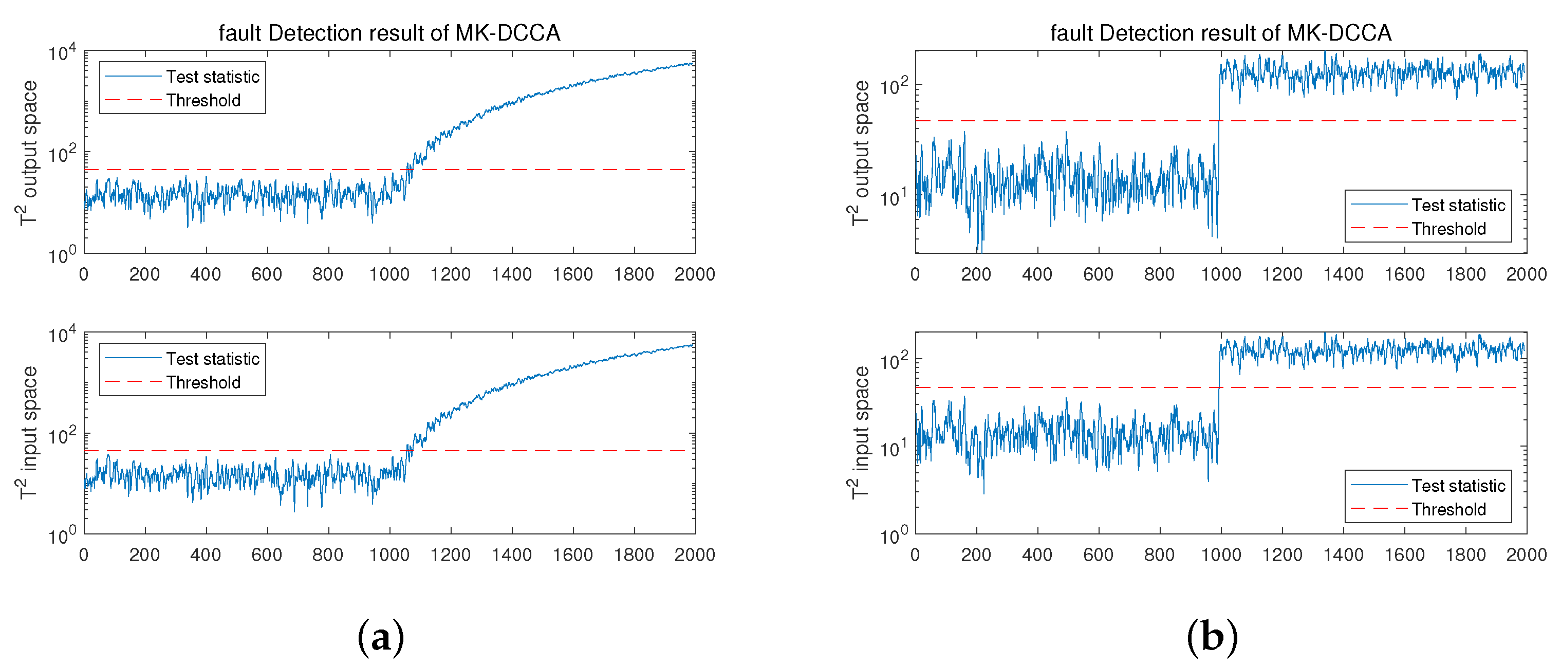
4.1.2. Process Monitoring

In this subsection, the fault-free dataset generated in Section 4.1.1 is employed as the training set to train the model. The fault datasets are then used as the test set for process monitoring to demonstrate the performance of the proposed method. The monitoring results for Fault 1 and Fault 2 are shown in Figure 1, separately.

The monitoring graphs reveal that the proposed approach effectively identifies the abnormal states of the system and provides early warnings. For Fault 1 (incipient fault), the monitoring model can provide an alert at the 54th sample after a fault occurs and effectively forecast evolving trends of faults. Moreover, for another prevalent fault, namely Fault 2 (abrupt fault), the monitoring model can promptly alert about an abnormal operating state of the system as soon as a fault occurs. Simultaneously, the proposed approach exhibits satisfactory performance during the monitoring processes of both aforementioned fault types. To comprehensively evaluate performance of the method, this study quantifies it using four metrics: fault detection rate (FDR), false alarm rate (FAR), miss detection rate (MDR), and fault detection time (FDT). FDT indicates the time when monitoring model initiates the first alert after a fault occurs. The definitions for the other three metrics are provided below:

$$\begin{array}{c}FDR=\frac{TP}{TP+FN}\\ FAR=\frac{FP}{FP+TN}\\ MDR=\frac{FN}{TP+FN}\end{array}$$

(52)

where $TP$ is the number of faults correctly detected, $TN$ represents the number of normals correctly detected, $FP$ denotes the number of normal samples incorrectly reported as faults, and $FN$ signifies the number of faults incorrectly reported as normals. Ultimately, utilizing the aforementioned metrics, the quantified results of monitoring performance are displayed in

Table 2. Monitoring performance indicators of Fault 1 and Fault 2.

Fault Index	Statistical Metrics	FDR(%)	FAR(%)	MDR(%)	FDT(s)
Fault 1	$T_{in}^2$	91.9	0	8.1	1054
	$T_{out}^2$	92.5	0	7.5	1054
Fault 2	$T_{in}^2$	99.9	0	0.1	1000
	$T_{out}^2$	99.9	0.1	0.1	1000

.

It is evident that the proposed approach achieves a fault detection rate of 92.5% for the incipient fault (Fault 1) and attains a higher 99.9% detection rate for the comparatively easily detectable abrupt fault (Fault 2). As for the false alarm rate, the MK-DCCA method maintains an excellent performance of zero false alarms for both fault types. Meanwhile, the proposed method successfully manages to maintain the miss detection rate at an acceptable level of 7.5% for Fault 1, whereas for the more readily detectable Fault 2, the miss detection rate decreases to 0.1%. Ultimately, the fault detection time for Fault 1 occurs at the 1054th sample (54 samples following the fault occurrence), while for Fault 2, it is the 1000th sample (immediately following the fault occurrence). The reason behind this phenomenon is that incipient faults exhibit a relatively minor impact on monitoring indicators during the early stages of fault occurrence, necessitating a certain degree of fault development to trigger model warnings.

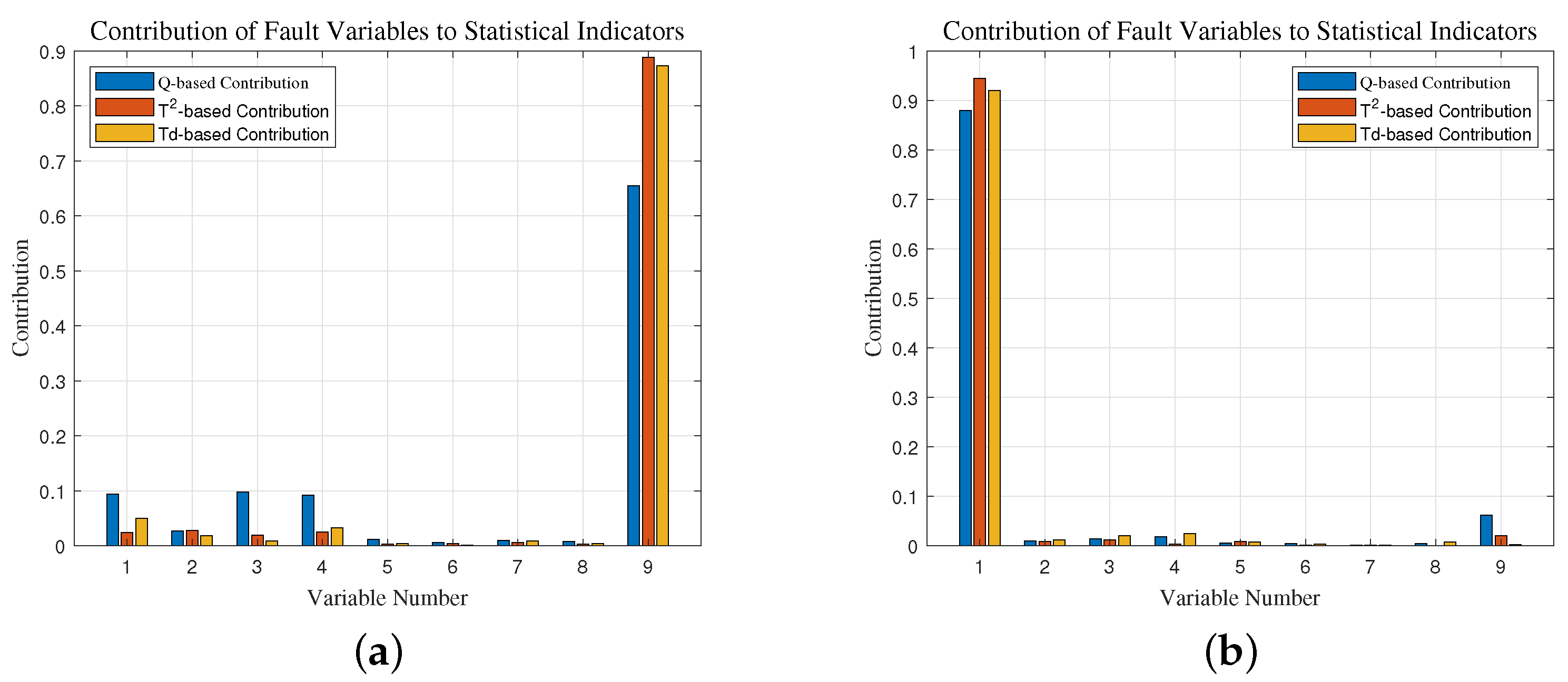
4.1.3. Fault Identification

This section of the experiment primarily aims to evaluate the fault identification capability of the proposed method. It involves identify the fault variables by evaluating the contribution of each variable to the fault detection indicators, with the goal of achieving accurate fault localization. The variable contribution plots of Fault 1 and Fault 2 are illustrated in Figure 2:

Table 1 indicates that the fault variable for Fault 1 is the 9th variable, while for Fault 2, it is the 1st variable. This conclusion is also apparent from Figure 2. It is evident that in both types of fault identification experiments, the $T^2$ indicator contribution performed the best. For Fault 1, variable 9 contributed 96.7% to the fault statistic indicator, while for Fault 2, variable 1 contributed 98.6%. Hence, the fault identification method employed in this research demonstrates a satisfactory level of accuracy.

In conclusion, the process monitoring and fault identification experiments conducted on a randomly generated dataset from a standard process model have demonstrated strong generalization performance of the proposed method. Simultaneously, it has exhibited satisfactory monitoring performance and fault identification accuracy.

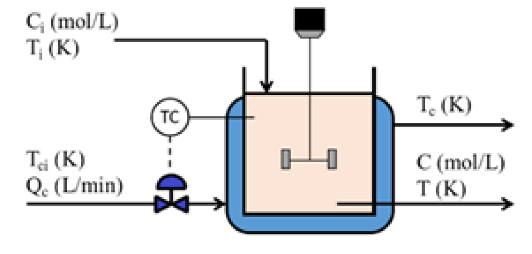
4.2. Case II: Case Analysis of CSTR Simulation Model

4.2.1. Model Introduction

The dataset employed in this case study is generated by a CSTR Simulink simulation model tailored for simulating incipient faults. A detailed description of the model can be found in [9]. The schematic diagram of the CSTR model is shown in Figure 3, and

Table 3. Process variables involved in the CSTR system.

Variable Index	1	2	3	4	5	6	7	8	9	10
Variable Name	$C_i$	$T_i$	$T_{ci}$	$C_i$	$T_i$	C	T	$T_c$	$T_{ci}$	$Q_c$1

¹ Variables 1 to 3 represent measurements without noise; this study utilizes variables 4 to 10.

summarizes all the process variables of the system. The system inputs are $C_i$, $T_i$, and $T_{ci}$, while the system outputs are C, T, $T_c$, and $Q_c$. The dynamic model of the CSTR process is described as follows:

$$\begin{array}{c}\frac{dC}{dt}=\frac{Q}{V}\left(C_i-c\right)-a_{1}kC+v_1\hfill \\ \frac{dT}{dt}=\frac{Q}{V}\left(T_i-T\right)-a_1\frac{\left(\Delta H_r\right)kC}{\rho C_{p}V}\left(T-T_c\right)+v_2\hfill \\ \frac{d{T}_c}{dt}=\frac{Q_c}{V_c}\left(T_{ci}-T_c\right)+b_1\frac{UA}{{\rho }_C{C}_{pc}{V}_c}\left(T-T_c\right)+v_3\hfill \end{array}$$

(53)

where Q is the inlet flow rate, $\Delta H_r$ is the heat of reaction, $UA$ is the heat transfer coefficient, $\rho$ and ${\rho }_C$ are the fluid density, $C_p$ and $C_{pc}$ are the heat capacity of the fluid, and V and $V_c$ are the volumes of the tank and jacket, respectively.

The training and testing sets were collected from the CSTR simulation model during a 1200 s run, with a sampling rate of one sample per second. Each testing set initiates from a fault-free state and introduces faults after running for 200 s. Four fault scenarios were employed to evaluate the effectiveness of the proposed method, including two input subspace faults and two output subspace faults, with detailed fault information provided in

Table 4. Fault detailed information.

Fault Index	Simulated Fault Scenario	Fault Variables	Fault Category	Introduction Time (s)	Associated Subspace
Fault 1	Feed valve malfunction	$C_i$	Incipient	200	Input
Fault 2	High coolant temperature	$T_{ci}$	Abrupt	200	Input
Fault 3	Coolant leakage	$Q_c$	Incipient	200	Output
Fault 4	High reactor temperature	T	Abrupt	200	Output
Fault 5	Both 1 and 3	$C_i$, $Q_c$	Incipient	200	/

.

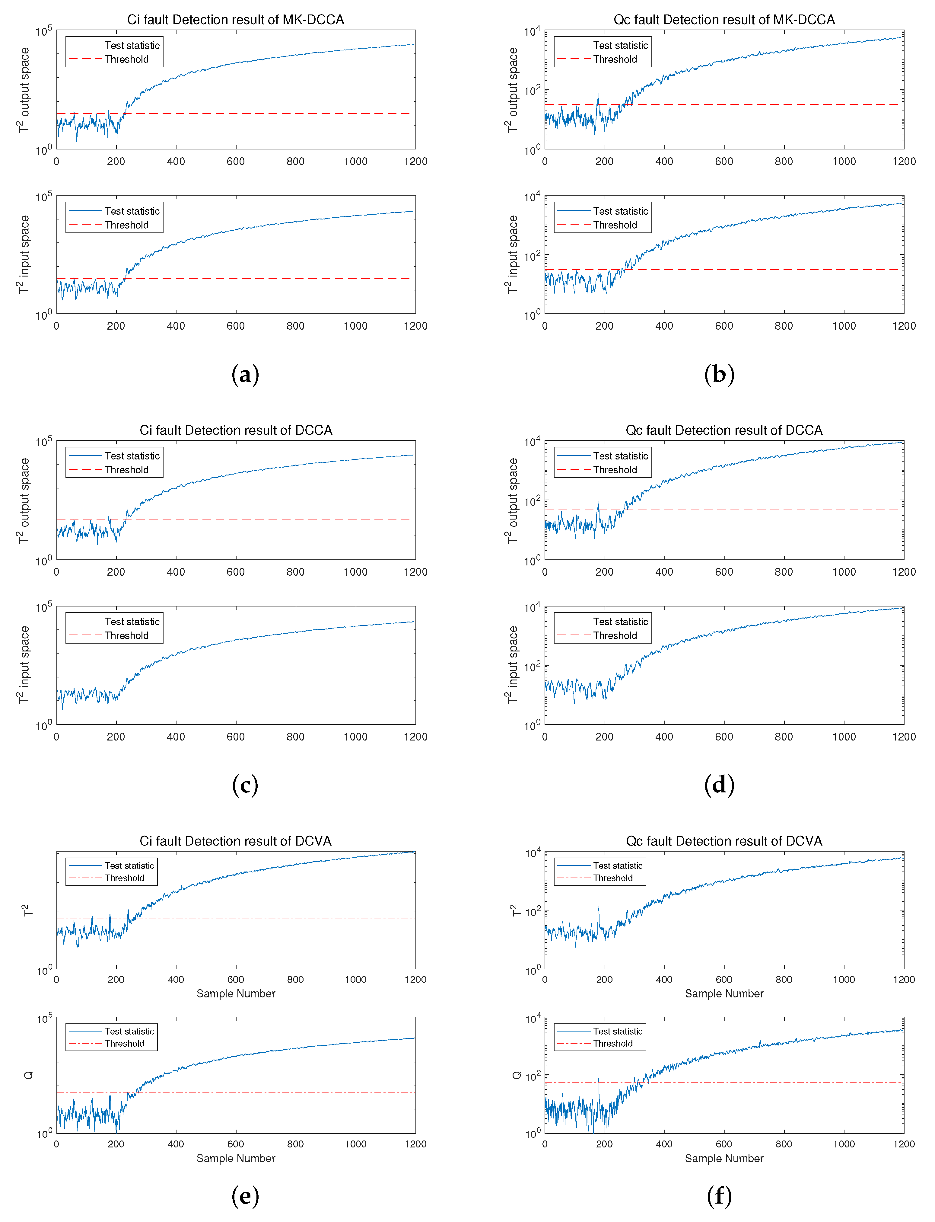
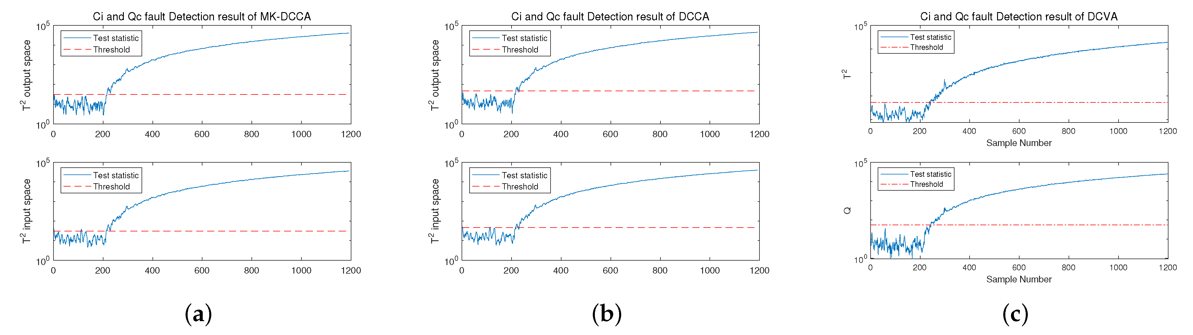
4.2.2. Process Monitoring

In this section, we initiate comparative experiments for the relatively easily detectable abrupt faults, faults 2 and 4. Subsequently, experiments are conducted on faults 1 and 3 (incipient faults), followed by the simultaneous introduction of both incipient faults of Fault 5 for detection. The methods employed include MK-DCCA, DCCA, and DCVA.

The process monitoring experimental results for faults 2 and 4 are illustrated in Figure 4.

From the graphs, it is evident that all three methods can provide early warnings for both Fault 2 and Fault 4 as they occur. However, in terms of false alarm rate, MK-DCCA exhibits the lowest, followed by DCCA, and DCVA performs the poorest. To facilitate better comparison of the three methods,

Table 5. Performance indicators for monitoring of faults 2 and 4 using different methods.

Fault Index	Method	Statistical Metrics	FDR(%)	FAR(%)	MDR(%)	FDT(s)
Fault 2	MK-DCCA	$T_{in}^2$	99.8	0	0.2	202
		$T_{out}^2$	100	0	0	200
	DCCA	$T_{in}^2$	99.9	0	0.1	201
		$T_{out}^2$	100	3.14	0	200
	DCVA	Q	99.5	1.05	0.5	205
		$T^2$	99.5	2.1	0.5	205
Fault 4	MK-DCCA	$T_{in}^2$	100	1.05	0	200
		$T_{out}^2$	100	2.62	0	200
	DCCA	$T_{in}^2$	100	2.62	0	200
		$T_{out}^2$	100	6.81	0	200
	DCVA	Q	99.5	3.66	0.5	205
		$T^2$	99.5	5.24	0.5	205

presents the detailed information of their monitoring performance indicators. The results demonstrate that both the MK-DCCA and DCCA methods achieve a fault detection rate of 100% for both faults 2 and 4, surpassing the DCVA method. Meanwhile, both the MK-DCCA and DCCA methods exhibit no false alarms in the monitoring of fault 2, whereas the DCVA method achieves the best performance with a false alarm rate of 1.05% based on the Q criterion. In experiments for Fault 4, the MK-DCCA method similarly achieves the lowest false alarm rate of 1.05%, followed by the DCCA method at 2.62%, and the DCVA method performs the least favorably with a rate of 3.66%. Furthermore, in terms of missed detection rate, both CCA-based methods maintained the lowest 0 missed detection rate in experiments for faults 2 and 4, while the DCVA method had a rate of 0.5%. Lastly, in comparison to the CVA-based method, the fault detection time of the CCA-based method is slightly reduced in both fault scenarios.

To conclude, in terms of abrupt fault detection, the proposed MK-DCCA method performs the best, followed by the DCCA method, and finally the CVDA method. Therefore, applying the proposed method for detecting abrupt faults in industrial process systems is justified in this study.

Furthermore, the study further compared and analyzed the monitoring performance of the proposed method and the comparative methods in the incipient fault scenarios of faults 1 and 3. The process monitoring experimental results for faults 1 and 3 are depicted in Figure 5.

The figures clearly illustrate that the MK-DCCA, DCCA, and DCVA methods all exhibit the ability to provide alerts after a certain time period following the occurrence of faults, and simultaneously, they are capable of predicting the trend of fault progression. However, in comparison, the MK-DCCA method still performs better and more comprehensively, and detailed analysis of performance indicators can be found in

Table 6. Performance indicators for monitoring of faults 2 and 4 using different methods.

Fault Index	Method	Statistical Metrics	FDR(%)	FAR(%)	MDR(%)	FDT(s)
Fault 1	MK-DCCA	$T_{in}^2$	96.204	5.24	3.80	223
		$T_{out}^2$	96.304	1.57	3.70	225
	DCCA	$T_{in}^2$	96.004	0	4.0	231
		$T_{out}^2$	96.004	3.14	4.0	231
	DCVA	Q	92.607	0	7.40	237
		$T^2$	93.506	3.14	6.50	236
Fault 3	MK-DCCA	$T_{in}^2$	93.007	0	7.0	246
		$T_{out}^2$	92.408	3.14	7.60	259
	DCCA	$T_{in}^2$	92.907	0	7.10	238
		$T_{out}^2$	92.907	2.62	7.10	260
	DCVA	Q	87.013	1.57	12.99	297
		$T^2$	91.009	2.09	8.99	271

. It is evident that the MK-DCCA method attains fault detection rates of 96.304% and 93.007% for the monitoring of fault 1 and fault 3, respectively, surpassing the FDR values of the DCCA and DCVA methods. Concurrently, in the fault scenarios of faults 1 and 3, the CCA-based approach can attain lower false alarm rates than the CVA-based approach. Additionally, in terms of missed detection rates, the MK-DCCA method maintains the lowest rates in the monitoring of both faults, at 3.7% and 7.0%, respectively. As for fault detection time, the CCA-based method significantly reduces detection time compared to the CVA-based method, although the DCCA method also exhibits shorter detection time than the MK-DCCA method, it comes at the cost of slightly higher false alarm rates, making the performance of MK-DCCA more satisfactory in comparison.

In summary, in experiments for detecting incipient faults, the MK-DCCA method proposed in this paper continues to exhibit the best performance, followed by the DCCA method, and finally the CVDA method. Accordingly, the performance of the proposed method has been demonstrated to be satisfactory in both abrupt fault and incipient fault detection scenarios. Additionally, in order to align the research more closely with complex real-world application scenarios, faults 1 and 3 were simultaneously introduced into the CSTR system, referred to as Fault 5. The detailed results of the fault detection experiment for Fault 5 are shown in Figure 6, and the specific values of the related performance indicators are presented in

Table 7. Performance indicators for monitoring of Fault 5 using different methods.

Method	Statistical Metrics	FDR(%)	FAR(%)	MDR(%)	FDT(s)
MK-DCCA	$T_{in}^2$	97.203	1.04	2.80	215
	$T_{out}^2$	97.403	0	2.60	216
DCCA	$T_{in}^2$	97.103	1.05	2.90	215
	$T_{out}^2$	97.303	0	2.70	216
DCVA	Q	94.805	0	5.19	243
	$T^2$	95.105	0	4.90	237

.

It is evident that the CCA-based method holds a notable advantage over the CVA-based method, exhibiting a higher detection rate by around 2%, a lower miss detection rate by approximately 2%, and a reduction in detection time by about 20 s. Simultaneously, in the comparison between MK-DCCA and DCCA methods, the former prevails with a slight advantage in detection rate and miss detection rate. This reasserts the excellence of the proposed MK-DCCA method and its feasibility in intricate application environments.

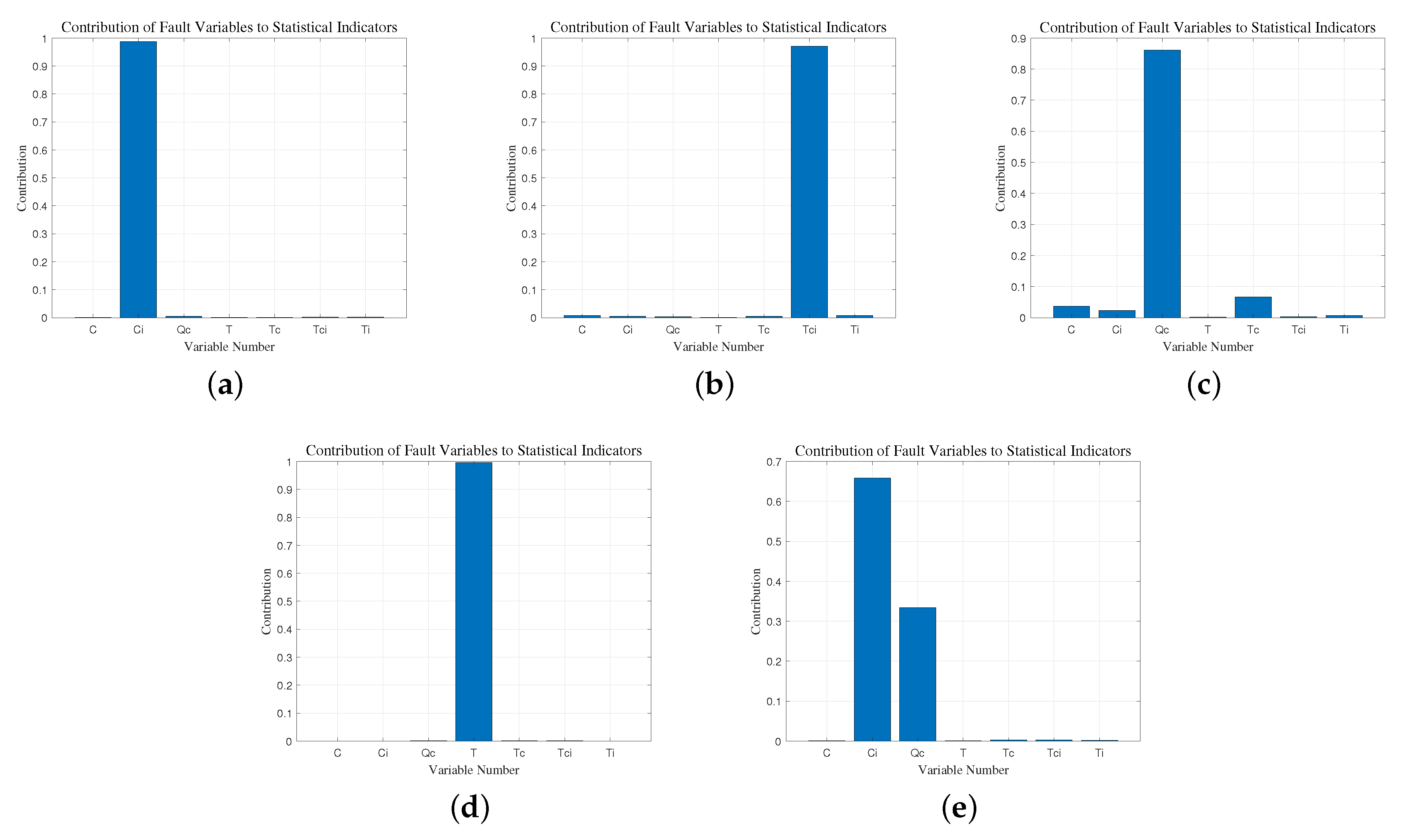
4.2.3. Fault Identification

In the previous section, the fault detection performance of the proposed method has been validated. In this section, the main emphasis lies in the analysis of fault identification capability of the method. Since it has been demonstrated in Section 4.1.3 that the $T^2$-based contribution identification accuracy is the highest, in experiments of this section, only the $T^2$-based contribution is used for fault identification. The contribution plots for faults 1 to 5 are shown in Figure 7.

It can be observed that in Fault 1, the variable $C_i$ contributes 98.66% to the statistical indicator, with the fact that $C_i$ is the actual fault variable; in faults 2, 3, and 4, the contributions of the fault variables $T_{ci}$, $Q_c$, and T are 97.52%, 86.32%, and 99.32%, respectively, far exceeding other variables; in Fault 5, which involves the fault variables $C_i$ and $Q_c$, their contributions are 64.3% and 34.84%, respectively, also significantly higher than other variables. The above findings demonstrate that the fault identification approach adopted in this study exhibits a satisfactory identification accuracy, effectively identifying and locating faults with precision.

5. Conclusions

This paper emphasizes the importance of detecting incipient faults in process industrial systems and extends the widely recognized process monitoring method, CCA, to make it more suitable for early detection of incipient faults. By incorporating time parameters, the method gains the ability to handle system dynamics. The inclusion of kernel methods endows the method with the capability to handle nonlinear data. In the selection of kernel functions, a weighted combination of RBF and polynomial kernels is chosen, allowing the kernel function to possess both good interpolation and extrapolation capabilities. Based on the aforementioned work, this paper proposes an MK-DCCA fault diagnosis method, and its generalization performance is validated on a randomly generated dataset, then comparative experiments are conducted on the CSTR Simulink model. The results demonstrate the superiority of the proposed method in fault detection, especially in the case of incipient faults, over the DCCA and DCVA methods.

Nevertheless, this study has certain limitations. The method requires a considerable number of parameters, and its performance is somewhat dependent on the selection of these parameters. The calculation of thresholds is relatively inflexible, leading to limited adaptability to different monitoring objects. Future research will aim to address these issues by exploring adaptive parameter selection and threshold computation. In addition, the hidden Markov model (HMM) method is mentioned in [35], by which the hidden Markov model (HMM) coupled with the Baum–Welsh algorithm can discover the hidden states that represent the precursors of the accidental events, which enables the system to better identify the fault precursors, which provides a new perspective for the study of early diagnosis of incipient faults. In future work, we also hope to conduct an in-depth comparative study of this method to propose a superior performance method for the early diagnosis of incipient faults.

References

1. Tang, M.; Yang, C.; Gui, W. Fault detection based on cost-sensitive support vector machine for alumina evaporation process. Control. Eng. China 2011, 18, 645–649. [Google Scholar]
2. Qin, S.J. Survey on data-driven industrial process monitoring and diagnosis. Annu. Rev. Control. 2012, 36, 220–234. [Google Scholar] [CrossRef]
3. Wise, B.M.; Gallagher, N.B. The process chemometrics approach to process monitoring and fault detection. J. Process. Control 1996, 6, 329–348. [Google Scholar] [CrossRef]
4. Tessier, J.; Duchesne, C.; Tarcy, G.; Gauthier, C.; Dufour, G. Analysis of a potroom performance drift, from a multivariate point of view. In Proceedings of the Light Metals-Warrendale-Proceedings—TMS, New Orleans, LO, USA, 9–13 March 2008; Volume 2008, p. 319. [Google Scholar]
5. Abd Majid, N.A.; Taylor, M.P.; Chen, J.J.; Stam, M.A.; Mulder, A.; Young, B.R. Aluminium process fault detection by multiway principal component analysis. Control. Eng. Pract. 2011, 19, 367–379. [Google Scholar] [CrossRef]
6. Ding, S.X.; Yin, S.; Peng, K.; Hao, H.; Shen, B. A novel scheme for key performance indicator prediction and diagnosis with application to an industrial hot strip mill. IEEE Trans. Ind. Inform. 2012, 9, 2239–2247. [Google Scholar] [CrossRef]
7. Harkat, M.F.; Mansouri, M.; Nounou, M.N.; Nounou, H.N. Fault detection of uncertain chemical processes using interval partial least squares-based generalized likelihood ratio test. Inf. Sci. 2019, 490, 265–284. [Google Scholar]
8. Ruiz-Cárcel, C.; Cao, Y.; Mba, D.; Lao, L.; Samuel, R. Statistical process monitoring of a multiphase flow facility. Control. Eng. Pract. 2015, 42, 74–88. [Google Scholar] [CrossRef]
9. Pilario, K.E.S.; Cao, Y. Canonical variate dissimilarity analysis for process incipient fault detection. IEEE Trans. Ind. Inform. 2018, 14, 5308–5315. [Google Scholar] [CrossRef]
10. Pilario, K.E.S.; Cao, Y.; Shafiee, M. Mixed kernel canonical variate dissimilarity analysis for incipient fault monitoring in nonlinear dynamic processes. Comput. Chem. Eng. 2019, 123, 143–154. [Google Scholar] [CrossRef]
11. Pilario, K.E.S.; Cao, Y.; Shafiee, M. Incipient Fault Detection, Diagnosis, and Prognosis using Canonical Variate Dissimilarity Analysis. Comput. Aided Chem. Eng. 2019, 46, 1195–1200. [Google Scholar]
12. Chen, Z.; Ding, S.X.; Zhang, K.; Li, Z.; Hu, Z. Canonical correlation analysis-based fault detection methods with application to alumina evaporation process. Control. Eng. Pract. 2016, 46, 51–58. [Google Scholar] [CrossRef]
13. Chen, Z.; Deng, Q.; Zhao, Z.; Tang, P.; Luo, W.; Liu, Q. Application of just-in-time-learning CCA to the health monitoring of a real cold source system. IFAC-PapersOnLine 2022, 55, 23–30. [Google Scholar] [CrossRef]
14. Chen, Z.; Zhang, K.; Ding, S.X.; Shardt, Y.A.; Hu, Z. Improved canonical correlation analysis-based fault detection methods for industrial processes. J. Process. Control 2016, 41, 26–34. [Google Scholar] [CrossRef]
15. Gao, L.; Li, D.; Yao, L.; Gao, Y. Sensor drift fault diagnosis for chiller system using deep recurrent canonical correlation analysis and k-nearest neighbor classifier. ISA Trans. 2022, 122, 232–246. [Google Scholar] [CrossRef] [PubMed]
16. Li, X.; Wang, Y.; Tang, B.; Qin, Y.; Zhang, G. Canonical correlation analysis of dimension reduced degradation feature space for machinery condition monitoring. Mech. Syst. Signal Process. 2023, 182, 109603. [Google Scholar] [CrossRef]
17. Chen, Z.; Liang, K. Canonical correlation analysis–based fault diagnosis method for dynamic processes. In Fault Diagnosis and Prognosis Techniques for Complex Engineering Systems; Elsevier: London, UK, 2021; pp. 51–88. [Google Scholar]
18. Pilario, K.E.; Shafiee, M.; Cao, Y.; Lao, L.; Yang, S.H. A Review of Kernel Methods for Feature Extraction in Nonlinear Process Monitoring. Processes 2020, 8, 24. [Google Scholar] [CrossRef]
19. Cheng, H.; Liu, Y.; Huang, D.; Cai, B.; Wang, Q. Rebooting kernel CCA method for nonlinear quality-relevant fault detection in process industries. Process. Saf. Environ. Prot. 2021, 149, 619–630. [Google Scholar] [CrossRef]
20. Cheng, H.; Wu, J.; Huang, D.; Liu, Y.; Wang, Q. Robust adaptive boosted canonical correlation analysis for quality-relevant process monitoring of wastewater treatment. ISA Trans. 2021, 117, 210–220. [Google Scholar] [CrossRef]
21. Liu, Q.; Zhu, Q.; Qin, S.J.; Chai, T. Dynamic concurrent kernel CCA for strip-thickness relevant fault diagnosis of continuous annealing processes. J. Process. Control 2018, 67, 12–22. [Google Scholar] [CrossRef]
22. Yu, J.; Yang, Z.; Zhou, L.; Ye, L.; Song, Z. A Novel Dynamic Baysian Canonical Correlation Analysis Method for Fault Detection. IFAC-PapersOnLine 2020, 53, 13707–13712. [Google Scholar] [CrossRef]
23. Chen, Q.; Wang, Y. Key-performance-indicator-related state monitoring based on kernel canonical correlation analysis. Control. Eng. Pract. 2021, 107, 104692. [Google Scholar] [CrossRef]
24. Zhu, Q.; Liu, Q.; Qin, S.J. Concurrent monitoring and diagnosis of process and quality faults with canonical correlation analysis. IFAC-PapersOnLine 2017, 50, 7999–8004. [Google Scholar] [CrossRef]
25. Huang, Z.-J.; Yuan, S.-J.; Li, D.-S.; Li, H.-N. A kernel canonical correlation analysis approach for removing environmental and operational variations for structural damage identification. J. Sound Vib. 2023, 548, 117516. [Google Scholar] [CrossRef]
26. Amorosi, L.; Padellini, T.; Puerto, J.; Valverde, C. A Mathematical Programming Approach to Sparse Canonical Correlation Analysis. Expert Syst. Appl. 2024, 237, 121293. [Google Scholar] [CrossRef]
27. Luo, L.; Wang, W.; Bao, S.; Peng, X.; Peng, Y. Robust and sparse canonical correlation analysis for fault detection and diagnosis using training data with outliers. Expert Syst. Appl. 2024, 236, 121434. [Google Scholar] [CrossRef]
28. Schölkopf, B.; Smola, A.; Müller, K.R. Nonlinear component analysis as a kernel eigenvalue problem. Neural Comput. 1998, 10, 1299–1319. [Google Scholar] [CrossRef]
29. Smola, A.; Ovári, Z.; Williamson, R.C. Regularization with dot-product kernels. Adv. Neural Inf. Process. Syst. 2000, 13, l308–1314. [Google Scholar]
30. Cristianini, N.; Shawe-Taylor, J. An Introduction to Support Vector Machines and Other Kernel-Based Learning Methods; Cambridge University Press: Cambridge, UK, 2000. [Google Scholar]
31. Negiz, A.; Çlinar, A. Statistical monitoring of multivariable dynamic processes with state-space models. AIChE J. 1997, 43, 2002–2020. [Google Scholar] [CrossRef]
32. Li, X.; Mba, D.; Diallo, D.; Delpha, C. Canonical variate residuals-based fault diagnosis for slowly evolving faults. Energies 2019, 12, 726. [Google Scholar] [CrossRef]
33. Jiang, B.; Huang, D.; Zhu, X.; Yang, F.; Braatz, R.D. Canonical variate analysis-based contributions for fault identification. J. Process. Control 2015, 26, 17–25. [Google Scholar] [CrossRef]
34. Jordaan, E. Development of Robust Inferential Sensors: Industrial Applications of Support Vector Machines for Regression. Ph.D. Thesis, Eindhoven University of Technology, Eindhoven, Holland, 2002. [Google Scholar] [CrossRef]
35. Vairo, T.; Pettinato, M.; Reverberi, A.P.; Milazzo, M.F.; Fabiano, B. An approach towards the implementation of a reliable resilience model based on machine learning. Process. Saf. Environ. Prot. 2023, 172, 632–641. [Google Scholar] [CrossRef]
Figure 1. Monitoring results of the randomly generated dataset by MK-DCCA: (a) Monitoring results for Fault 1. (b) Monitoring results for Fault 2.
Processes 11 02927 g001
Figure 2. Contribution plot of process variables under fault scenarios: (a) Contribution plot of Fault 1. (b) Contribution plot of Fault 2.
Processes 11 02927 g002
Figure 3. Schematic diagram of the CSTR model.
Processes 11 02927 g003
Figure 4. Monitoring results for faults 2 and 4 by three methods: (a) Monitoring results of MK-DCCA approach for Fault 2. (b) Monitoring results of MK-DCCA approach for Fault 4. (c) Monitoring results of DCCA approach for Fault 2. (d) Monitoring results of DCCA approach for Fault 4. (e) Monitoring results of DCVA approach for Fault 2. (f) Monitoring results of DCVA approach for Fault 4.
Processes 11 02927 g004
Figure 5. Monitoring results for faults 1 and 3 by three methods: (a) Monitoring results of MK-DCCA approach for Fault 1. (b) Monitoring results of MK-DCCA approach for Fault 3. (c) Monitoring results of DCCA approach for Fault 1. (d) Monitoring results of DCCA approach for Fault 3. (e) Monitoring results of DCVA approach for Fault 1. (f) Monitoring results of DCVA approach for Fault 3.
Processes 11 02927 g005
Figure 6. Monitoring results for Fault 5 by three methods: (a) Monitoring results of MK-DCCA. (b) Monitoring results of DCCA. (c) Monitoring results of DCVA.
Processes 11 02927 g006
Figure 7. Monitoring results for Fault 5 by three methods: (a) Contribution plot of variables for Fault 1. (b) Contribution plot of variables for Fault 2. (c) Contribution plot of variables for Fault 3. (d) Contribution plot of variables for Fault 4. (e) Contribution plot of variables for Fault 5.
Processes 11 02927 g007