Research on Optimal Scheduling of Multi-Energy Microgrid Based on Stackelberg Game

Abstract

In recent years, rapid industrialization has driven higher energy demand, depleting fossil-fuel reserves and causing excessive emissions. China’s “dual carbon” strategy aims to balance development and sustainability. This study optimizes microgrid efficiency with a tiered carbon-priced economy. A Stackelberg game establishes microgrid-user equilibrium, solved iteratively with a multi-population algorithm (MPGA). Comparative analysis can be obtained without considering demand response scenarios, and the optimization cost of microgrid operation considering price-based demand response scenarios was reduced by 5%; that is 668.95 yuan. In addition, the cost of electricity purchase was decreased by 23.8%, or 778.6 yuan. The model promotes user-driven energy use, elevating economic and system benefits, and therefore, the scheduling expectation of “peak shaving and valley filling” is effectively realized.

1. Introduction

With the rapid development of modern industry, the contradiction between energy consumption and the environment has become increasingly prominent, and the large emission of greenhouse gases has led to a more severe ecological environment and more serious global warming: according to the BP World Energy Statistical Yearbook 2022 [1], global primary energy consumption in 2021 showed a rebound trend, an increase of nearly 6%. This significantly reversed the sharp decline in energy consumption due to lockdowns in many countries around the world in 2020. Therefore, all countries are seeking energy transformation, and any successful and long-lasting energy transformation cannot be separated from the three elements: safety, burden, and low-carbon. Therefore, countries have formulated corresponding emission reduction targets, focusing on policy incentives and government economic investment as the main body to achieve excessive excess of traditional energy to low-carbon energy. In the daily production and consumption process led by electricity as a high-quality energy source, according to the theoretical guidance of “high energy, high energy, low energy and low-use, temperature-oriented, step use”, the three-energy coupling of electricity–heat–gas are explored and improved energy conversion. The new way of rate, especially the utilization of thermal energy, has achieved results in the energy terminal. As a large country of energy use, China strives to achieve carbon peaks by 2030 and achieve carbon neutralization by 2060 [2]. In order to achieve the ambitions and commitments of decarburization and achieve promise, China must establish a relatively sound energy system, with the development of clean energy as the guide, and take the first step in the transformation of China’s energy industry structure [3].

In recent years, many scholars have conducted a lot of research on the optimization of the comprehensive energy system. Zhou Nan and others introduced the time-sharing pricing strategy into the optimization scheduling of energy storage to maximize the annual profit and utilization rate of photovoltaic systems [4]. Li Xiulei et al. established a general model for energy storage and demand response optimization planning, and analyzed the impact of energy storage and demand response on goals in operational strategies. The end of the energy cycle in demand response is usually thermal energy, so the main coupling method is the electrical thermal component, and the load type mainly exists in the form of temperature-controlled loads. However, due to its inherent limitations, thermal energy is often strongly influenced by external weather factors and has a delay effect. Therefore, through research on modeling, optimization, and control of electrical thermal coupling components, its impact on power system stability can be reduced [5]. Wang Dan et al. provided an energy-saving design for temperature-controlled loads in buildings, while considering the limitations of user comfort to determine the operating method of the power plant, and established the optimal allocation model for energy-saving power plants [6]. Wang Chengshan et al. used a simplified equivalent thermodynamic model with first-order parameters and a state control model to smooth out renewable energy in microgrids by replacing energy storage technology with demand side and load response technology [7]. Tang Xiaoting et al. constructed a mathematical model that includes input and output energy balance constraints of energy hubs, system capacity constraints, and energy storage efficiency constraints of renewable energy generation technology [8]. Heiskanin et al. Proposed the Energy System Analysis Environmental Assessment Framework (EAFESA) [9]. This framework can minimize the shortcomings of the two models and maximize the combination of the two models to analyze the no climatic environmental impacts of energy scenarios based on the life cycle. Wu Yong et al. established a multi-objective optimization model for comprehensive planning of various energy storage capacities with the goal of minimizing economic costs and network carbon emissions, but did not consider the impact of different energy storage components on the system [10]. Zhang Xizheng searched algorithm (GSA) and particle swarm optimization (PSO) algorithm by combining gravitational, a hybrid modified GSA-PSO (MGSA-PSO) scheme is proposed to optimize the load dispatch of the microgrid containing electric vehicles. The load dispatch optimization are implemented and analyzed, including the unordered charging strategy, the ordered charging–discharging strategy, and the ordered charging–discharging strategy with distributed generations [11]. Zhang Feng et al. applied a robust ALO optimizer (ALO) algorithm for MPP tracking of solar photovoltaic system, designed the charge controller of the energy storage system, and designed the DC–AC converter to match the frequency of RES with the frequency of DG [12].

In summary, due to the continuous improvement of energy coupling in microgrids and the continuous reform of the electricity market, the mathematical models of equipment in microgrids have increased, and operation scheduling strategies have become more complex. Traditional control methods for loads need to be reformed. In addition, in the context of huge carbon emissions, carbon reduction and environmental benefits cannot be achieved in parallel. Therefore, this article conducts reasonable scheduling of devices in microgrids, seeks more reasonable and economical device matching methods, introduces a demand response mechanism, constructs a low-carbon economic optimization model for microgrids with tiered carbon prices, and establishes a Stackelberg game model to control user load, achieving the goal of “peak shaving and valley filling”, which is of great significance for the overall energy utilization of microgrids.

Considering the multi-energy micro-network planning process under the carbon trading mechanism, there are many stakeholders during energy transactions: the distribution network–microcyllar network and user side. In order to meet the demands of various interests at the same time, the main game framework was introduced. At the same time, because there is an energy interaction between the distribution network and the microcontrollers, the relationship between the energy demand response and the user’s side has the relationship between the micro grid and the user. That is to say, on the upper layer of the main game, the microblogs are maximized to the system’s efforts to maximize the effort of the system according to the price signal given by the distribution network. To participate in the scheduling for the goal, and to obtain a balanced solution, micro-network response strategies through price demand can guide users to participate in micro-network scheduling can achieve energy transition. As the main body of energy use, the spontaneous use of the electricity price incentive signal transfer period or cut load based on the spontaneous operator’s electricity price incentive signal can be used to achieve the goal of peak-cutting the valley of the load of the microblog.

Therefore, this article proposes a multi-energy microfinance low-carbon tone considering the main game, and the establishment of the overall micro-power grid.

This article does the following:

• A low-carbon economic optimization model of microgrid with tiered carbon price was constructed. The carbon emissions involved in the operation of each equipment are finally traded through the carbon trading market, and the sensitivity analysis of the system is carried out by adjusting the ladder carbon trading parameters.
• A Stackelberg game model with microgrid as the main body of the game and user response as the follower of the game was established, which further improved the level of load participation in the energy system and proved the existence of equilibrium solutions in the game. The model is iteratively solved by a variety of group algorithms, and immigration operators and artificial selection operators are added to the traditional genetic algorithm to prevent all individuals in the population from tending to the same state and stop evolution, and at the same time increase the memory population and improve the model calculation efficiency.

2. Optimization Model of Micro-Grid Low-Carbon Economy with Ladder Carbon Price

2.1. Stepped Carbon Trading Model

Carbon emission quota trading can limit the amount of carbon emissions according to specific emission industries. At the same time, the real-time price of the carbon market is determined by the carbon trading market, and the carbon emission quota is managed in a reasonable and efficient way [13].

2.1.1. Calculation Model of Carbon Emissions

The main carbon sources in microgrid are power consumption process, heat generation and power generation process of cogeneration unit, gas-fired boiler, and coal-fired unit. Because the coal-fired units are equipped with carbon capture power plants, it can help the microgrid consume part of $\mathrm{C}{\mathrm{O}}_2$. Therefore, when calculating the actual carbon emissions, the $\mathrm{C}{\mathrm{O}}_2$ absorbed by the carbon capture equipment needs to be removed. The total carbon emission model of microgrid is shown in Formula (1), and the total amount of gas purchased is shown in Formula (2).

$$\begin{array}{c}{E}_{all}={\lambda }_e{\displaystyle \sum _{t=1}^T}{P}_{e,buy}+{\lambda }_g{\displaystyle \sum _{t=1}^T}{P}_{g,buy}+Q_{C{O}_2}^{PGU}-{\displaystyle \sum _{t=1}^T}{Q}_{C{O}_2}^{CCS}\end{array}$$

(1)

$$\begin{array}{c}{P}_{g,buy}=P_{g,CHP}+P_{g,GB}\end{array}$$

(2)

$P_{e,buy}$, $P_{g,buy}$ are purchase electricity and gas, ${\lambda }_e$, ${\lambda }_g$ are carbon emission coefficients of electricity-consuming equipment and gas-consuming equipment, $Q_{C{O}_2}^{PGU}$ is emissions for coal-fired power plants $\mathrm{C}{\mathrm{O}}_2$ quantity, and $Q_{C{O}_2}^{CCS}$ is the amount of carbon capture equipment $\mathrm{C}{\mathrm{O}}_2$.

2.1.2. Carbon Decentralization Quota Model

The initial allocation of carbon emission rights in this paper mainly includes electricity purchase quota, cogeneration unit quota, gas boiler quota, and coal-fired power plant quota. The carbon emission quota model for power purchase in microgrid is shown in Formula (3), and the model synthesis of cogeneration unit, gas boiler, and coal-fired power plant is shown in Formula (4).

$$\begin{array}{c}{E}_e={\epsilon }_e{\displaystyle \sum _{t=1}^T}{P}_{e,buy}\end{array}$$

(3)

$$\begin{array}{c}{E}_x={\epsilon }_x\cdot P_x\end{array}$$

(4)

${\epsilon }_e$, ${\epsilon }_x$ are carbon emission quotas for unit electric power and unit power consumed by different equipment.

2.1.3. Stepped Carbon Trading Model

Based on the above carbon emission model and carbon emission rights allocation model, a ladder carbon trading model is established, and a plurality of carbon emission rights purchase intervals are set in the ladder carbon trading mechanism. The initial carbon emission quota allocated by the system is removed from the total carbon emission, and the mathematical Formula is shown in Formula (5). At the same time, pricing with different gradients is carried out according to the net carbon emission of the system in different charging intervals, when the net carbon emission is less than a given interval length. In the internal time, only the transaction amount at the base price of carbon trading is paid. When the price is higher than a given interval length, the price in each step interval is fixed. Every step increase, the carbon trading price increases exponentially, the carbon emission right purchase ratio increases, and the corresponding price will also increase. According to this trading model, the mathematical model Formula of ladder carbon trading as shown in Formula (6) is obtained.

$$\begin{array}{c}E=E_{all}-E_e-{\displaystyle \sum _i^N}{E}_x\end{array}$$

(5)

$$C_{C{O}_2}=\left\{\begin{array}{l}c\cdot E,E\le l\\ c\cdot \left(1+\lambda \right)\left(E-l\right)+cl,l\le E\le 2l\\ c\cdot \left(1+2\lambda \right)\left(E-2l\right)+c\left(2+\lambda \right)l,2l\le E\le 3l\\ c\cdot \left(1+3\lambda \right)\left(E-3l\right)+c\left(3+3\lambda \right)l,3l\le E\le 4l\\ c\cdot \left(1+4\lambda \right)\left(E-4l\right)+c\left(4+6\lambda \right)l,E\ge 4l\end{array}\right.$$

(6)

$C_{C{O}_2}$ is carbon transaction costs, $E$ is carbon emission of the system, $i$ is equipment selection, including cogeneration units, gas-fired boilers and coal-fired power plants, $N$ is the total number of device, $\lambda$ is the price growth rate, $l$ is the interval length, $c$ is the base price of carbon trading.

2.2. Microgrid Low-Carbon Economic Optimization Model with Step Carbon Price

Based on the established carbon trading mechanism, a low-carbon optimization model of microgrid with ladder carbon trading mechanism is proposed. The model considers the lowest comprehensive operating cost of the whole microgrid from the economic level, implements the initial carbon emission quota form from the environmental level, and comprehensively considers the operating cost, system power consumption cost, gas consumption cost, and carbon trading cost of the whole system exceeding the carbon emission quota. The electric balance, thermal balance, gas balance and hydrogen balance in the overall operation of the system are taken as equality constraints, and the climbing constraints and output upper limit constraints of each device are taken as inequality constraints, so as to improve the economy and low carbon of the microgrid [14].

2.2.1. Objective Function

The overall objective function of microgrid not only minimizes the fuel cost and the cost of purchasing electricity and gas, but also supplements the environmental problems according to the carbon trading mechanism. Among them, the carbon transaction cost is the ladder carbon price cost considering exceeding the carbon emission quota. On the premise of ensuring the safety and reliability of the whole microgrid system, the environmental factors are quantified, and the output degree of each micro-source is optimized according to the load change, so as to obtain the minimum comprehensive cost of the system.

$$\begin{array}{c}\mathit{min}F=\mathit{min}{\displaystyle \sum _{t=1}^T}\left(C_{PGU}+C_{e,buy}+C_{g,buy}+C_{C{O}_2}\right)\end{array}$$

(7)

$F$ is the minimum operate cost of the system, $C_{PGU}$ is fuel costs, $C_{e,buy}$ is the cost of electricity purchase, $C_{g,buy}$ is gas purchase cost, and $C_{C{O}_2}$ is carbon transaction costs.

• Fuel cost

$$\begin{array}{c}{C}_{pgu}=a{p}_{PGU}^2+b{p}_{PGU}+c\end{array}$$

(8)

b.

Energy purchase cost

$$\begin{array}{c}{C}_{e,buy}+C_{g,buy}=c_e{\sum }_{t=1}^T{P}_{e,buy}+c_g{\sum }_{t=1}^T{P}_{g,buy}\end{array}$$

(9)

$P_{e,buy}$ is the total power consumption of the system, $P_{g,buy}$ is the total gas consumption of the system, $c_e$ is real-time electricity prices, $c_g$ is real-time gas price, and $T$ takes 24 h.

2.2.2. System Operation Constraints

According to the law of conservation of energy, when the microgrid is running as a whole, the output energy of each form should always be equal to the input energy of each form to maintain the system operation. At the same time, the output energy of each equipment is kept within the rated power and cannot exceed the specified maximum output, so the related mathematical Formulas of balance constraint and imbalance constraint in the system are integrated, respectively.

The equality constraints are as follows:

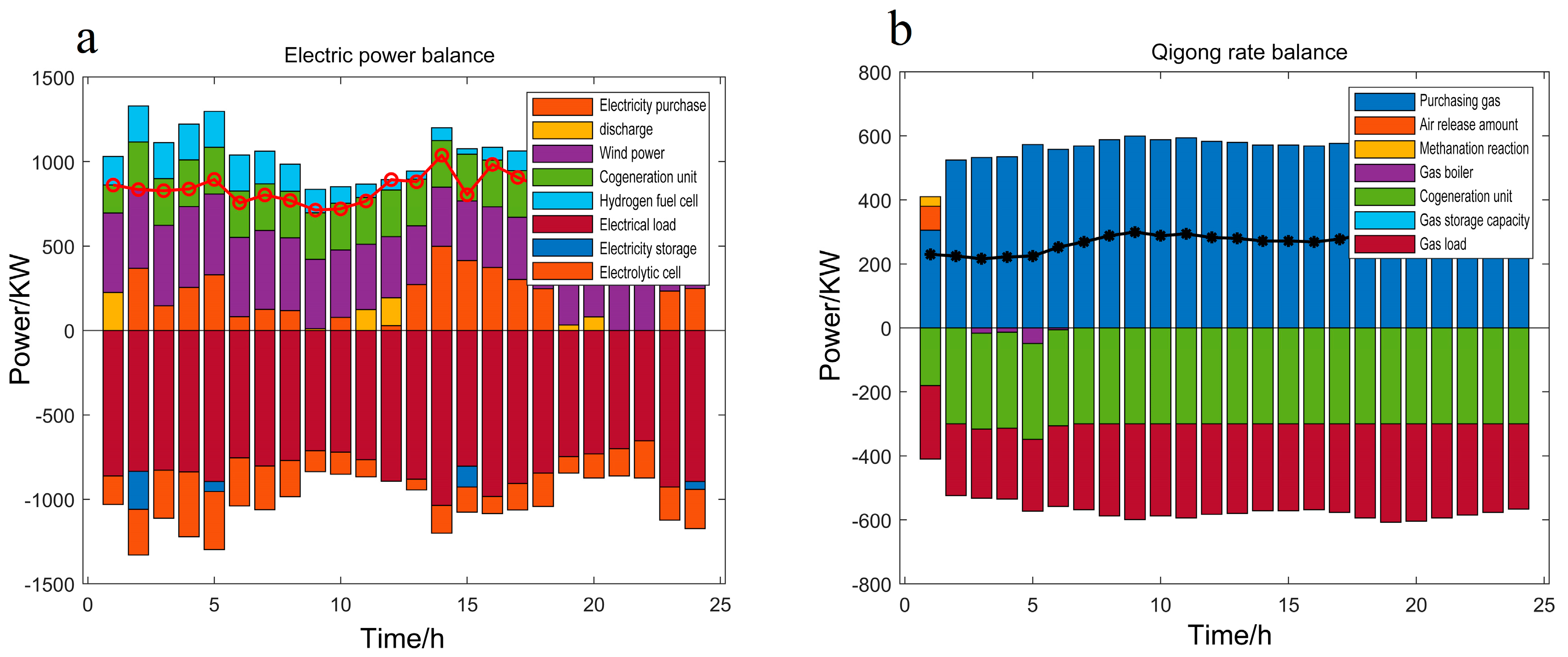
• Electric power balance

On the premise of ignoring the network loss, the discharge of wind power, cogeneration units, and power storage equipment, the purchase of electricity from the superior power grid and the overall output of hydrogen fuel cells are equal to the sum of the electric power consumed by the electric load and the charging of power storage equipment, as shown in Formula (10).

$$\begin{array}{c}{P}_{WT}\left(t\right)+P_{CHP}\left(t\right)+P_{SB,dis}\left(t\right)+P_{e,buy}\left(t\right)+P_{HFC,e}\left(t\right)=P_{load}\left(t\right)+P_{SB,chr}\left(t\right)\end{array}$$

(10)

$P_{WT}\left(t\right)$ is output power for wind energy, $P_{CHP}\left(t\right)$ is output power for electric energy of cogeneration unit, $P_{SB,dis}\left(t\right)$ is the discharge power for electric storage device, $P_{HFC,e}\left(t\right)$ is electricity production of hydrogen fuel cell, $P_{load}\left(t\right)$ is the electrical load, and $P_{SB,chr}\left(t\right)$ is charging the power storage equipment.

b.

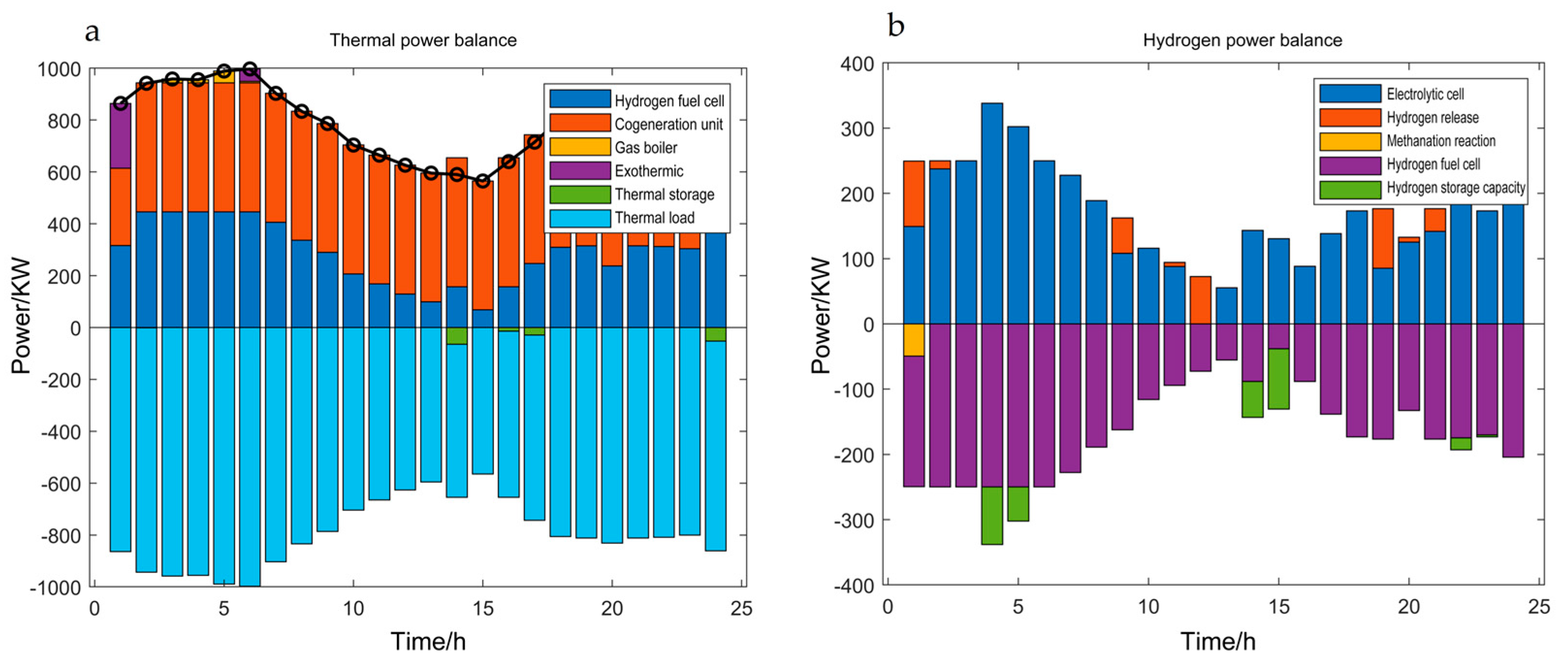
Thermal power balance

The input heat of the system is equal to the output heat; that is, the sum of the exothermic power of cogeneration unit, gas boiler, and heat storage equipment is equal to the thermal power consumed by heat storage equipment and heat load.

$$\begin{array}{c}{P}_{HFC,h}\left(t\right)+H_{CHP}\left(t\right)+H_{GB}\left(t\right)+H_{TS,dis}\left(t\right)=H_{TS,chr}\left(t\right)+H_{Load}\left(t\right)\end{array}$$

(11)

$H_{CHP}\left(t\right)$ the thermal energy output power of the cogeneration unit, $H_{GB}\left(t\right)$ is the heat generation of gas boilers, $H_{TS,dis}\left(t\right)$ is released for the heat storage device, $H_{TS,chr}\left(t\right)$ is the heat release of heat storage equipment, and $H_{Load}\left(t\right)$ is the heat load.

c.

Natural gas power balance

Similarly, the output of natural gas is equal to the input, that is, the sum of gas purchase, gas storage tank, gas release, and gas conversion technology output is equal to the gas load, gas storage tank, gas storage, cogeneration unit, and gas boiler gas consumption.

$$\begin{array}{c}{G}_{buy}\left(t\right)+G_{ES,dis}\left(t\right)+G_{MR}\left(t\right)=G_{load}+G_{ES,chr}\left(t\right)+G_{CHP}\left(t\right)+G_{GB}\left(t\right)\end{array}$$

(12)

$G_{buy}\left(t\right)$ is the amount of gas purchased, $G_{ES,dis}\left(t\right)$ is the amount of gas vented by the gas receiver, $G_{MR}\left(t\right)$ is the amount of ${CH}_4$ dioxide produced by methanation of electricity-to-gas technology, $G_{load}$ is gas load, $G_{ES,chr}\left(t\right)$ is the gas storage capacity of the gas storage equipment, $G_{CHP}\left(t\right)$ is the air consumption of the cogeneration unit, and $G_{GB}\left(t\right)$ is the amount of natural gas consumed by the gas boiler unit.

d.

Hydrogen power balance

Because the two steps of electro-gas conversion technology in microgrid are modeled separately and equipped with hydrogen storage tank and hydrogen fuel cell, hydrogen energy balance is added.

$$\begin{array}{c}{P}_{EL,H_2}\left(t\right)+P_{HS,dis}\left(t\right)=P_{H_2,MR}\left(t\right)+P_{H_2,HFC}\left(t\right)+P_{HS,chr}\left(t\right)\end{array}$$

(13)

$P_{EL,H_2}\left(t\right)$ is the hydrogen production capacity of the electrolytic cell in the first step of converting electricity to gas, $P_{HS,dis}\left(t\right)$ is the hydrogen storage capacity of the hydrogen storage device, $P_{H_2,MR}$ is the hydrogen consumption of methanation reaction, $P_{H_2,HFC}$ is the hydrogen consumption of the hydrogen fuel cell, $P_{HS,chr}\left(t\right)$ is amount of hydrogen released for hydrogen storage equipment.

Inequality constraints are as follows:

• Coal-fired units

During the operation of coal-fired units, it is necessary to ensure that the output is within the allowable range, that is, to ensure the output constraint.

$$\begin{array}{c}{P}_{PGU}^{min}\le P_{PGU}\le P_{PGU}^{max}\end{array}$$

(14)

$P_{PGU}^{max}$ and $P_{PGU}^{min}$ are the upper and lower limits of the output of coal-fired units.

The output adjustment of coal-fired units should be within the allowable range, that is, climbing constraint.

$$\begin{array}{c}\Delta P_{PGU}^{min}\le \Delta P_{PGU}\le \Delta P_{PGU}^{max}\end{array}$$

(15)

$$\begin{array}{c}\Delta P_{PGU}^{min}\le \Delta P_{PGU}\le \Delta P_{PGU}^{max}\end{array}$$

(16)

$\Delta P_{PGU}^{max}$ is the maximum upward climb power of the coal-fired unit, $\Delta P_{PGU}^{min}$ is the maximum downward climb power of the coal-fired unit, $\Delta P_{PGU}$ is the amount of power change, $P_{PGU}\left(t\right)$ is the power of the coal-fired unit at the time of t, $P_{PGU}\left(t-1\right)$ is the power of the coal-fired unit at the time of t − 1.

b.

Cogeneration unit

Because the cogeneration unit meets both the electric load and the heat load, it needs to meet both the electric output constraint and the heat output constraint.

$$\begin{array}{c}{P}_{CHP,e}^{min}\le P_{CHP,e}\le P_{CHP,e}^{max}\end{array}$$

(17)

$$\begin{array}{c}{H}_{CHP,h}^{min}\le H_{CHP,h}\le H_{CHP,h}^{max}\end{array}$$

(18)

$P_{CHP,e}^{max}$ and $P_{CHP,e}^{min}$ are the upper and low limits of the electric output of the cogeneration unit, $H_{CHP,h}^{min}$ and $H_{CHP,h}^{max}$ are the upper and lower limits of thermal output of cogeneration unit.

Climbing constraints are shown in Formulas (19) and (20).

$$\begin{array}{c}\Delta P_{convert,e}^{min}\le \Delta P_{convert,e}\le \Delta P_{convert,e}^{max}\end{array}$$

(19)

$$\begin{array}{c}\Delta P_{convert,e}=P_{convert,e}\left(t\right)-P_{convert,e}\left(t-1\right)\end{array}$$

(20)

$\Delta P_{convert,e}^{max}$ is the maximum upward climb power of that cogeneration unit, $\Delta P_{convert,e}^{min}$ is the maximum downward climb power of the cogeneration unit, $\Delta P_{convert,e}$ is the amount of power change under the pure condensation condition, $P_{convert,e}\left(t\right)$ is the electrical power of the cogeneration unit after the t time conversion, $P_{convert,e}\left(t-1\right)$ is the electrical power of the cogeneration unit after the t − 1 time conversion.

c.

Electro-gas conversion technology

The electrolyzer and methanation reaction should meet the hydrogen production output constraint and the $C{H}_4$ output constraint, respectively.

$$\begin{array}{c}{P}_{EL,H_2}^{min}\le P_{EL,H_2}\le P_{EL,H_2}^{max}\end{array}$$

(21)

$$\begin{array}{c}{G}_{MR}^{min}\le G_{MR}\le G_{MR}^{max}\end{array}$$

(22)

$P_{EL,H_2}^{max}$ and $P_{EL,H_2}^{min}$ are the upper and lower limits of hydrogen production by the electrolyzer, $G_{MR}^{max}$ and $G_{MR}^{min}$ are the upper and lower limits of the $C{H}_4$ quantity obtained by the reaction.

Climbing constraints are shown in Formulas (23)–(26).

$$\begin{array}{c}\Delta P_{EL,H_2}^{min}\le \Delta P_{EL,H_2}\le \Delta P_{EL,H_2}^{max}\end{array}$$

(23)

$$\begin{array}{c}\Delta P_{EL,H_2}=P_{EL,H_2}\left(t\right)-P_{EL,H_2}\left(t-1\right)\end{array}$$

(24)

$$\begin{array}{c}\Delta G_{MR}^{min}\le \Delta G_{MR}\le \Delta G_{MR}^{max}\end{array}$$

(25)

$$\begin{array}{c}\Delta G_{MR}=G_{MR}\left(t\right)-G_{MR}\left(t-1\right)\end{array}$$

(26)

$\Delta P_{EL,H_2}^{max}$ and $\Delta G_{MR}^{max}$ is the maximum upward climb power of that electrolytic cell and methanation reaction, $\Delta P_{EL,H_2}^{min}$ and $\Delta G_{MR}^{min}$ are the electrolyzer and methanation reaction large downward climb power, $\Delta P_{EL,H_2}$ and $\Delta G_{MR}$ are the amount of power change, $P_{EL,H_2}\left(t\right)$ and $G_{MR}\left(t\right)$ are the power of the electrolyzer and methanation reaction at the time of t, $P_{EL,H_2}\left(t-1\right)$ and $G_{MR}\left(t-1\right)$ are the power of the electrolyzer and methanation reaction at the time of t − 1.

d.

Gas-fired boiler unit

The output constraint and climbing constraint of gas-fired boilers are similar to those of coal-fired units, as shown in Formulas (27)–(29).

$$\begin{array}{c}{H}_{GB}^{min}\le H_{GB}\le H_{GB}^{max}\end{array}$$

(27)

$$\Delta \begin{array}{c}{H}_{GB}^{min}\le \Delta H_{GB}\le \Delta H_{GB}^{max}\end{array}$$

(28)

$$\begin{array}{c}\Delta H_{GB}=H_{GB}\left(t\right)-H_{GB}\left(t-1\right)\end{array}$$

(29)

$H_{GB}^{max}$ and $H_{GB}^{min}$ are the upper and lower limits of gas boiler output, $\Delta H_{GB}^{min}$ is the maximum upward climbing power of the gas boiler, $\Delta H_{GB}^{min}$ is the maximum downward climbing power of the gas boiler, $\Delta H_{GB}$ is the amount of power change, $H_{GB}\left(t\right)$ is the gas boiler power at the time of t, $H_{GB}\left(t-1\right)$ is the gas boiler power at the time of t.

e.

Hydrogen fuel cell

Similarly, the output constraints and climbing constraints of hydrogen fuel cells are shown in Formulas (30)–(32).

$$\begin{array}{c}{P}_{HFC,e}^{min}\le P_{HFC,e}\le P_{HFC,e}^{max}\end{array}$$

(30)

$$\begin{array}{c}\Delta P_{HFC,e}^{min}\le \Delta P_{HFC,e}\le \Delta P_{HFC,e}^{max}\end{array}$$

(31)

$$\begin{array}{c}\Delta P_{HFC,e}=P_{HFC,e}\left(t\right)-P_{HFC,e}\left(t-1\right)\end{array}$$

(32)

$P_{HFC,e}^{max}$ and $P_{HFC,e}^{min}$ are the upper and lower limits of hydrogen fuel cell output, $\Delta P_{HFC,e}^{max}$ is the maximum upward climb power of the hydrogen fuel cell, $\Delta P_{HFC,e}^{min}$ is the minimum upward climb power of the hydrogen fuel cell, $\Delta P_{HFC,e}$ is the amount of power change, $P_{HFC,e}\left(t\right)$ is the hydrogen fuel cell power at the time of t, $P_{HFC,e}\left(t-1\right)$ is the hydrogen fuel cell power at the time of t − 1.

3. Game Theory Basis

Gaming theory refers to the influence of the individual income of each participant in the case of the interdependence and interdependence of the participants. Therefore, because the income of all parties in the game receives the influence of multiple parties, each participant is considered to make rational judgments. Through the information obtained by themselves, they will give their strategies in real time to the overall feedback. The complete game consists of three basic elements:

3.1. Participants

Participants refer to the subjects that can Formulate strategies and make rational judgments in the overall game. Among them, the collection mathematics represents the participants (33).

$$\begin{array}{c}N=\left\{1,2,3,\dots ,n\right\}\end{array}$$

(33)

3.2. Strategy Set

Strategy is an important factor in the overall game. Participants have changed different strategies by collecting information, that is, the methods and means of maximizing their own interests to achieve their own interests. The number of strategies can be selected by themselves. Because the game is the mutual impact of the main body Formulation strategy, the sequence of the strategy Formulation has a huge impact on the results of the game. Among them, all participants Formulated the strategy collection mathematics indication (34).

$$\begin{array}{c}S=\left\{S_1,S_2,S_3,\dots S_n\right\}\end{array}$$

(34)

3.3. Effectiveness

The effect refers to the benefits that the participating entities of each game are after the game. Among them, benefits can be positive income or negative benefits, that is, the maximum benefits to obtain. The goal of the participants is to maximize the benefit by adjusting the strategy, and the benefit collection mathematical representation of the participants is shown in the math indication (35).

$$\begin{array}{c}u=\left\{u_1,u_2,u_3,\dots u_n\right\}\end{array}$$

(35)

After determining the basic three elements of the game, the establishment of a complete game is completed.

3.4. Stackelberg Game

Because the microgrid and the user side consider the price-based demand response, that is, there is no relevant agreement between the participants, users spontaneously change their energy consumption habits. Participants constantly adjust their own strategies to maximize their own interests during the scheduling process. There is still an obvious decision-making sequence between the microgrid and the client, with the microgrid acting first as the leader and the client following up as the follower. Among them, the leader first makes the appropriate decision, occupying the position of priority decision, and the follower makes the decision after receiving the signal from the leader. That is, microgrid is the leader to adjust the real-time price of distribution network, and the client is the follower to respond to the real-time price proposed by microgrid. This game type is called Stackelberg game. Stackelberg game is divided into dynamic non-cooperative game, also known as Stackelberg game. The model problems solved by the Stackelberg game mainly have the following characteristics [15]:

(1)

There is no agreement among the participants, and they make their own decisions.

(2)

The decision of each participant has an impact on the benefits of other participants.

(3)

Because of the different market positions, there is a decision-making order among the participants. The leader first makes appropriate decisions according to the target benefit, and the followers make decisions on their own goals after receiving the leader’s decision-making signal. There is a restrictive relationship between them.

(4)

The final decision-making scheme of each participant needs the unanimous consent of all participants.

The mathematical definition model of Stackelberg game is as follows:

Let the leader’s strategy set is $X$, the follower’s strategy set is $Y$, the leader’s utility function is $f:X\times Y\to R$, the utility function of the follower is $g:X\times Y\to R$.

As a dynamic game, leaders send out decision signals $x_n\in X$, followers make decisions according to the leader’s strategy, and the set of followers’ balance points is $A\left(x\right)$. Therefore, the mechanism mapping is generated: $X\to A\left(Y\right)$. When the next leader makes a decision, in order to maximize their own interests at all times, they will consider the follower scheme, and the overall game optimization goal is $maxf\left(x,y\right)$. Let $\left(x^{*},y^{*}\right)$ be the equilibrium point of the game, then the equilibrium condition is shown in Formula (4) [16].

$$\begin{array}{c}\left\{\begin{array}{c}\underset{x\in X}{max}f\left(x^{*},y^{*}\left(x^{*}\right)\right)\\ g\left(x^{*},y^{*}\right)\ge g\left(x^{*},y\right)\end{array}\right.\end{array}$$

(36)

4. Multi-Energy Microgrid Model Based on Stackelberg Game

4.1. The Demand Response Type

For the classification of electric energy demand response, the response method is mainly used as a differentiation method, both of which require a contract with the energy supply company, one is the price-based demand response, including time-of-use electricity price, real-time electricity price and peak electricity price. Compared with the incentive type, the price type has a lower degree of change in the user’s energy habits, and only needs to make voluntary adjustments to the price signal. The incentive-type response is to adjust the energy-using behavior strictly according to the load reduction calculation method and response time signed in the contract, and carry out the corresponding compensation mechanism for the adjusted energy-using behavior or impose corresponding fines for the part that does not meet the response requirements. Compared with the two corresponding methods, the current user acceptance of price-based demand response is higher, and the project implementation scope is wider, and this paper mainly studies price-based electricity price in the subsequent microgrid-user game stage.

The relationship model between electricity and electricity price is mainly divided into: electricity price elasticity matrix, user psychology model, exponential function fitting model, and statistical principle model [17]. Among them, the elasticity matrix of electricity and electricity prices is described as the change in electricity demand caused by the change in electricity price, and the elastic coefficient of electricity price is defined, and the calculation Formula is shown in Formula (37).

$$\begin{array}{c}\epsilon =\frac{\Delta P_e}{P_e}\frac{C_e}{\Delta C_e}\end{array}$$

(37)

In the Formula, $\Delta P_e$ is the amount of electricity increase, and $\Delta C_e$ is the increase in electricity price.

The electricity price response mechanism is divided into single period and multi-period, that is, fixed ladder electricity price and real-time electricity price, due to the peak and valley hours and price of the ladder electricity price is fixed, users will only change energy demand in a certain period, and real-time electricity price will prompt users to change energy consumption behavior according to different time periods. Therefore, a multi-period response mechanism is introduced, in which the multi-period elasticity coefficient is divided into the self-elasticity coefficient of the user response in the current period and the cross-elasticity coefficient of the user response behavior in other periods, and the mathematical model of the self-elasticity coefficient and cross-elasticity coefficient obtained according to the above definition is shown in Formulas (38) and (39).

$$\begin{array}{c}{\epsilon }_{ii}=\frac{\Delta P_i}{P_i}\frac{C_i}{\Delta C_i}\end{array}$$

(38)

$$\begin{array}{c}{\epsilon }_{ij}=\frac{\Delta P_i}{P_i}\frac{C_j}{\Delta C_j}\end{array}$$

(39)

In the Formula, ${\epsilon }_{ii}$ is the self-elastic coefficient and ${\epsilon }_{ij}$ is the cross-elastic coefficient. $i$ is the $i$th dispatch period and $j$ is the $j$th dispatch period.

According to the definition of the above elasticity coefficient and the mathematical model, the user price response model of the overall period is obtained as shown in Formula (40) and the electricity price elasticity matrix as shown in Formula (41)

$$\left[\begin{array}{c}\frac{\Delta C_1}{C_1}\\ \frac{\Delta C_2}{C_2}\\ ⋮\\ \frac{\Delta C_n}{C_n}\end{array}\right]=E\left[\begin{array}{c}\frac{\Delta P_1}{P_1}\\ \frac{\Delta P_2}{P_2}\\ ⋮\\ \frac{\Delta P_n}{P_n}\end{array}\right]$$

(40)

$$\begin{array}{c}E=\left[\begin{array}{cccc}{\epsilon }_{11}& {\epsilon }_{12}& \cdots & {\epsilon }_{1n}\\ {\epsilon }_{21}& {\epsilon }_{22}& \dots & {\epsilon }_{2n}\\ ⋮& ⋮& \ddots & ⋮\\ {\epsilon }_{n1}& {\epsilon }_{n2}& \dots & {\epsilon }_{nn}\end{array}\right]\end{array}$$

(41)

$\Delta C_n$ is the change in electricity price at $n$ moments after the demand response, $\Delta P_n$ is the load change at $n$ times after the demand response, $P_n$ is the load before the $n$ time response.

4.2. Microgrid-User Stackelberg Game Structure

As the leader in the Stackelberg game, microgrids generate revenue by developing pricing strategies different from those of distribution networks, selling electricity to users at different energy purchase prices [18,19]. Users, as followers in the Stackelberg game relationship, formulate a decision plan to reduce the cost of electricity purchase, that is, increase the amount of load transfer to reduce the cost of electricity purchase, and achieve the maximization of the follower’s benefits, that is, the maximum value of the follower’s objective function, as shown in Formula (51). Then, the scheme obtained by changing the load transfer amount is transmitted to the microgrid, which makes the next optimal decision based on the user’s response results. At this point, the output plan of the microgrid may not match the user’s demand, thereby reducing the maximum profit of the microgrid. Therefore, at this point, the microgrid will redesign its output plan and energy prices to achieve the highest return on the microgrid, which is the maximum value of the leader’s objective function, as shown in Formula (42). The Stackelberg game structure of microgrids is shown in Figure 1.

4.3. Microgrid Revenue Model

As the leader in the game, microgrid should achieve the optimal scheduling strategy of microgrid operation as a whole [20,21], set the price of electricity sales within 24 h in combination with the load change given by the user, realize the highest income, and construct the optimal operation income scheduling model of components of microgrid as a whole.

4.3.1. Objective Function

S is the minimum operating cost of the system in the game model, $C_{es,buy}$ is the cost of purchasing electricity from the superior power grid in the game model, $C_{eu,sell}$ is the electricity price income sold by microgrid to users, $C_{gs,buy}$ is the cost of buying gas, $C_{C{O}_2,s}$ is that transaction cost of carbon in the game model, $e_{es,buy}$ is the unit price of selling electricity for the distribution network, $e_{eu,sell}$ is the amount of electricity purchased for the microgrid, $P_{es,buy}$ is the electricity purchased by the user sold by the microgrid, $P_{user}$ is the amount of power after the user responds.

$$\begin{array}{c}minS=min{\displaystyle \sum _{t=1}^T}\left(C_{es,buy}-C_{eu,sell}+C_{gs,buy}+C_{C{O}_2,s}\right)\end{array}$$

(42)

$$\begin{array}{c}{C}_{es,buy}=e_{es,buy}{P}_{es,buy}\end{array}$$

(43)

$$\begin{array}{c}{C}_{eu,sell}=e_{eu,sell}{P}_{user}\end{array}$$

(44)

4.3.2. Constraints

Due to the introduction of the demand response mechanism, the upper and lower limits of the microgrid’s power purchase from the distribution network and the upper and lower limits of the microgrid’s selling price to users are increased, in which the power balance is shown in Formula (47). Thermal power balance, natural gas power balance, and hydrogen power balance are shown in the Formulas (12)–(14). The operating models, contribution models, and climbing models of thermoelectric units are as follows (17)–(20). The two-stage operation model, the power model, and the climbing model of the electrical rotation technology are as follows (21)–(26). The power boiler crew and the climbing models are shown in the Formulas (27)–(29), respectively. Hydrogen fuel cell operation models, contribution models, and climbing models are shown in the Formulas (30)–(32).

$$\begin{array}{c}{P}_{es,buy}^{min}\le P_{es,buy}\le P_{es,buy}^{max}\end{array}$$

(45)

$$\begin{array}{c}{e}_{eu,sell}^{min}\le e_{eu,sell}\le e_{eu,sell}^{max}\end{array}$$

(46)

$P_{es,buy}^{min}$ and $P_{es,buy}^{max}$ are the upper and lower limits of the amount of electricity that the microgrid purchases from the distribution network, $e_{eu,sell}^{max}$ and $e_{eu,sell}^{min}$ are the upper and lower limits of electricity price sold by microgrid to users.

$$\begin{array}{c}{P}_{WT}\left(t\right)+P_{CHP}\left(t\right)+P_{SB,dis}\left(t\right)+P_{e,buy}\left(t\right)+P_{HFC,e}=P_{user}\left(t\right)+P_{SB,chr}\left(t\right)\end{array}$$

(47)

$P_{WT}\left(t\right)$ is output power for wind energy, $P_{CHP}\left(t\right)$ is output power for electric energy of cogeneration unit, $P_{SB,dis}\left(t\right)$ is discharge power for that electric storage device, $P_{HFC,e}\left(t\right)$ is electricity production of hydrogen fuel cell, $P_{SB,chr}\left(t\right)$ is charging the power storage equipment.

Due to the introduction of price-based demand response, the relevant constraints of demand response should be increased. First, it is required that the total amount of load in the whole dispatching period remains unchanged, as shown in Formulas (48) and (49). At the same time, in order to achieve the ultimate goal of demand response, it is necessary to control the load of each step in the scheduling between the upper and lower limits of the load value before response, as shown in Formula (50).

$$\begin{array}{c}{\sum }_{t=1}^T\Delta P_{user,t}=0\end{array}$$

(48)

$$\begin{array}{c}\begin{array}{c}\Delta P_{user,t}=P_{user,t}^0-P_{user,t}\end{array}\end{array}$$

(49)

$$\left\{\begin{array}{c}{P}_{user,t}^{max}\le P_{user,t}^{0,max}\\ P_{user,t}^{min}\ge P_{user,t}^{0,min}\end{array}\right.$$

(50)

$\Delta P_{user,t}$ is the change in user electricity consumption before and after demand response, $P_{user,t}^0$ is the electricity consumption of users before demand response, $P_{user,t}^{0,max}$ and $P_{user,t}^{0,min}$ are the upper and lower limits of the demand response preload value, $P_{user,t}^{max}$ and $P_{user,t}^{min}$ are the upper and lower limits of the demand response afterload value.

4.4. User Benefit Model

User benefit refers to the reasonable adjustment of required energy according to its own demand for electricity and energy price in the process of demand response [22]. In this paper, the user satisfaction model is introduced to constrain the load variation. While considering the microgrid to guide users to adjust their own energy consumption period, the satisfaction of power consumption mode and expenditure satisfaction are used as constraints to participate in dispatching.

4.4.1. Objective Function

As a follower of the game, the user responds after the price signal is given by the microgrid. Considering the user’s power consumption income and cost, the goal is to maximize the user’s benefit, and the objective function is shown in Formula (51).

$$\begin{array}{c}maxU=C_{UE}-C_{eu,sell}\end{array}$$

(51)

$$\begin{array}{c}{C}_{UE}=\alpha \log \left(1+P_{user,t}\right)\end{array}$$

(52)

$U$ is that maximum benefit of user in the game model, $C_{UE}$ is the benefit of users, $\mathsf{\alpha }$ is energy preference coefficient for users.

4.4.2. Constraints

• Satisfaction with electricity consumption mode

Before the introduction of electricity price demand response, users’ electricity consumption periods were mainly selected according to their own preferences, and at this time, users’ satisfaction with electricity consumption methods was the highest [23]. However, after the introduction of electricity price demand response, the user changes his own electricity preference to reduce electricity expenditure by responding to the price signal given by the microgrid. The mathematical model is shown in Formula (53) and the satisfaction constraint is shown in Formula (54).

$$\begin{array}{c}M=1-\frac{{\sum }_{t=1}^T\left|\Delta P_{user,t}\right|}{{\sum }_{t=1}^T{P}_{user,t}^0}\end{array}$$

(53)

$$\begin{array}{c}M\ge M_{min}\end{array}$$

(54)

$M_{min}$ is the lower limit of user’s satisfaction with electricity consumption.

b.

Expenditure satisfaction

After the price-based demand response is implemented in the microgrid, users will adjust according to the real-time electricity price to ensure that the electricity expenditure will not have a great impact [24]. Therefore, expenditure satisfaction is usually used to measure the change in user expenditure. The mathematical model is shown in Formula (55), and the satisfaction constraint is shown in Formula (56).

$$\begin{array}{c}N=1+\frac{{\sum }_{t=1}^T(e_{eu,sell}^0{P}_{user,t}^0-e_{eu,sell}{P}_{user,t})}{e_{eu,sell}{P}_{user,t}}\end{array}$$

(55)

$$\begin{array}{c}N\ge N_{min}\end{array}$$

(56)

In the Formula, $e_{eu,sell}^0$ is the unit price of electricity sales for microgrid before demand response, $P_{user}^0$ is power consumption of users before demand response. $N_{min}$ is the lower limit of user spend satisfaction.

4.5. Establishment and Proof of Microgrid-Client Stackelberg Game

As shown in Figure 2, the microgrid and the user constitute a dynamic non-cooperative game, and the game relationship constitutes a Stackelberg game Formula as shown in Formula (57).

$$\begin{array}{c}G=\left\{\left(MGO\cup USER\right);{\Phi }_{MGO};{\Psi }_{USER};S_{MGO};U_{USER}\right\}\end{array}$$

(57)

Formula (52) contains three elements of the game: participants, strategy sets, and utility.

• Game participants: participants in the game of microgrid and users as the main slave, expressed in the form of set as follows $\left(MGO\cup USER\right)$.
• Strategy set: The microgrid is the leader in the Stackelberg game and the optimization strategy is Formulated first, and the electricity price strategy proposed by the microgrid to the user is represented by the set ${\Phi }_{MGO}$. The set of load adjustment strategies made by the user is represented by set ${\Psi }_{USER}$.
• Utility: The cost set of the microgrid is represented by set $S_{MGO}$, and the benefit set of users is represented by $U_{USER}$. the cost collection of microgrid.

When the follower in the game responds to the leader’s strategy, and the leader accepts the response, it shows that the upper and lower game as a whole has reached the equilibrium condition [24]. That is, when the user responds to the electricity price strategy proposed by the microgrid according to the optimized operation scheme, and the microgrid accepts the response strategy, the microgrid-user reaches the equilibrium condition. Make ${\Phi }_{MGO}^{*}$ a vector set representing all optimal strategies of a microgrid, and ${\Psi }_{USER}^{*}$ a vector set representing all the response strategies of the client. To reach the Stackelberg equilibrium condition, Formula (58) must be satisfied.

$$\left\{\begin{array}{l}{S}_{MGO}\left({\Phi }_{MGO}^{*},{\Psi }_{USER}^{*}\right)\ge S_{MGS}\left({\Phi }_x,{\Phi }_{n-x}^{*},{\Psi }_{USER}^{*}\right)\\ U_{USER}\left({\Phi }_{MGO}^{*},{\Psi }_{USER}^{*}\right)\ge U_{USER}\left({\Phi }_{MGO}^{*},{\Psi }_y,{\Psi }_{n-y}^{*}\right)\\ \forall {\Phi }_x\in {\Phi }_{MGO}\\ \forall {\Psi }_y\in {\Psi }_{USER}\end{array}\right.$$

(58)

${\Phi }_x$ is the optimal operation scheme of the microgrid, ${\Psi }_y$ is the optimal response scheme of the user terminal, ${\Phi }_{n-x}^{*}$ is yeah, except ${\Phi }_x$ other strategies than, ${\Psi }_{n-y}^{*}$ yeah, and except ${\Psi }_y$ other strategies outside.

In the equilibrium state of Stackelberg game, neither party can obtain greater benefits by unilaterally proposing new strategies, and it is necessary to verify the existence and uniqueness of the equilibrium solution before solving it. The theorems for verifying the existence of the equilibrium solution are as follows:

• The decision schemes of leaders and followers are all non-empty bounded convex sets;
• After the top leaders make decisions, the followers have corresponding unique solutions;
• After the lower followers respond, the leader has a unique solution.

Compared with the above definitions, the existence and uniqueness of Stackelberg equilibrium solution of microgrid-user Stackelberg game model established in this chapter are proved:

• As shown in Formulas (46) and (50), the policy set ${\Phi }_{MGO}$ and ${\Psi }_{USER}$ are non-null bounded convex set;
• As shown in Formulas (52)–(54), each term in $S_{MGO}$ is a linear or constant function with respect to $P_{es,buy}$ or $P_{user}$, then $S_{MGO}$ is a concave function with respect to $P_{es,buy}$ and $P_{user}$.
• As shown in Formulas (51) and (52), $U_{USER}$ is a continuous function with respect to $P_{es,buy}$ and $P_{user}$.

5. The Solution Method of Game Model Based on Multi-Population Genetic Algorithm

The previous chapter analyzed the energy flow relationship between devices in the microgrid and the optimization functions of various game entities, and established a Stackelberg game model for the microgrid user. As the function to be solved is a large-scale linear programming problem, compared to other algorithms, using multiple population genetic algorithms can effectively reduce the complexity of the solution and improve the efficiency of the solution.

Genetic Algorithm (GA) is an adaptive global optimization probability search algorithm proposed by Professor Holland in the United States in 1975 that simulates the genetic evolution of biological organisms in nature. Organisms evolve through heredity, variation, and natural selection, and genetic algorithms are inspired by Darwin’s theory of natural selection. The solution of the example corresponds to the chromosomes in the genetic process, and the set of all chromosomes is a population, and the individuals are eliminated between the populations according to the principle of “natural selection, survival of the fittest”, and the selection between individuals in the corresponding population is in programming. Starting from the initialization of the population, the interval judgment of the fitness function is carried out for each generation of the population, and according to the designed fitness ratio, the appropriate strategy is selected to select the excellent individuals of the current population, and the selected excellent individuals are crossed and mutated to form a new population. Analogous to the evolution process of species, generation-by-generation, continuously enhancing the fitness of the population until the optimal solution is output after the desired conditions are completed. Since the genetic algorithm does not rely on gradient calculation, it has strong robustness and global optimization ability [24,25].

Multi-population genetic algorithm divides a single population into multi-threaded populations and adds immigration operators. In the evolution process of different populations, the migration operator introduces the optimal individuals to other populations every certain number of iterations, which realizes the information exchange between different populations and the balance of global and local search performance. Secondly, the elite population is established, and each generation of evolution selects the best individuals of other populations to join the elite population and save them through artificial selection operators, and no genetic operation is carried out to ensure that the best individuals are not destroyed, so all the optimal solutions produced by each evolution can be completely preserved [26,27,28,29]. The simplified process of improvement is shown in Figure 3.

The solution process for the whole game system is as follows:

(1)

Initializing the operation parameters of the microgrid and the load data of the user terminal, and sending the electricity price strategy drawn up by the microgrid to the lower layer;

(2)

Converting the maximum energy consumption benefit of the user terminal into a negative cost, feeding back according to the pricing signal of the microgrid, and feeding back the load signal to the upper-level dispatching;

(3)

The microgrid solves the objective function through the feedback signal;

(4)

Judging whether the game equilibrium solution is reached, and if so, outputting the result; otherwise, return to (2) to continue scheduling.

6. Example Analysis

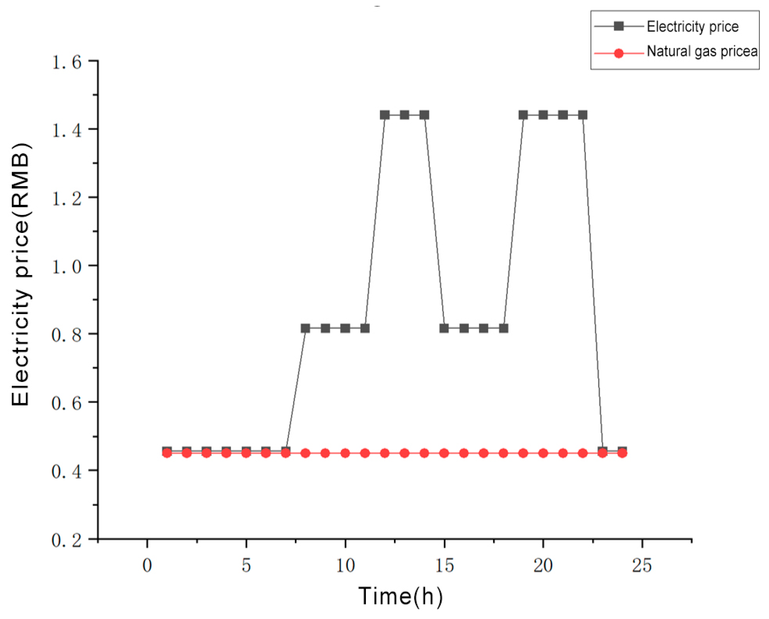
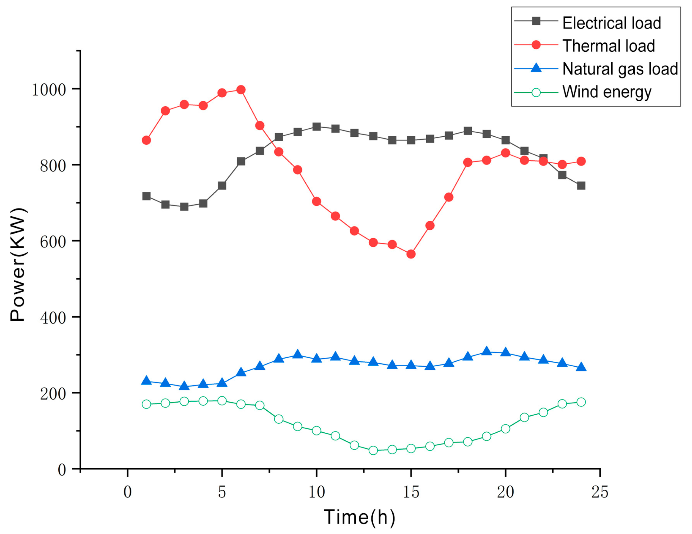
6.1. Basic Data

The reaction parameters of each equipment are shown in

Table 1. Operating parameters of each device.

Equipment	Value	Efficiency/Carbon Emissions Quota	Value
Carbon capture power plant contribution range/kw$·$h	[0, 200]	${\eta }_{CHP}$	0.92
The range of thermal power union crew/kw$·$h	[0, 300]	${\eta }_{EL}$	0.88
Thermoelectrician Unit is a thermal power ratio	1.8	${\eta }_{MR}$	0.6
The range of electrolytic tank equipment/kw$·$h	[0, 500]	${\eta }_{HFC}$	0.85
Methane reaction force range/kw$·$h	[0, 250]	${\epsilon }_e$	0.798
Hydrogen fuel cell contribution range/kw$·$h	[0, 250]	${\epsilon }_h$	0.985

. The electricity price and natural gas price are shown in Figure 3, but considering the price-based user demand response, the initial tiered price is adopted as shown in Figure 4, and the new demand response parameter data are shown in

Table 2. Demand Response Related Parameters.

Parameter Name	Value	Parameter Name	Value
$M_{min}$	0.9	${\epsilon }_{ii}$	−0.2
$N_{min}$	0.9	${\epsilon }_{ij}$	0.033

[30]. The typical electricity load, heat load, and gas load curves of the multi energy microgrid, as well as the predicted output power of wind power generation, are shown in Figure 5. Peak and valley time of use electricity prices are used for billing, with low peak periods ranging from 23.00 to 7.00, flat peak periods ranging from 8.00 to 11.00 and 15.00 to 18.00. Daytime peak periods are reached from 12.00 to 14.00, and nighttime peak periods are reached from 19.00 to 22.00.

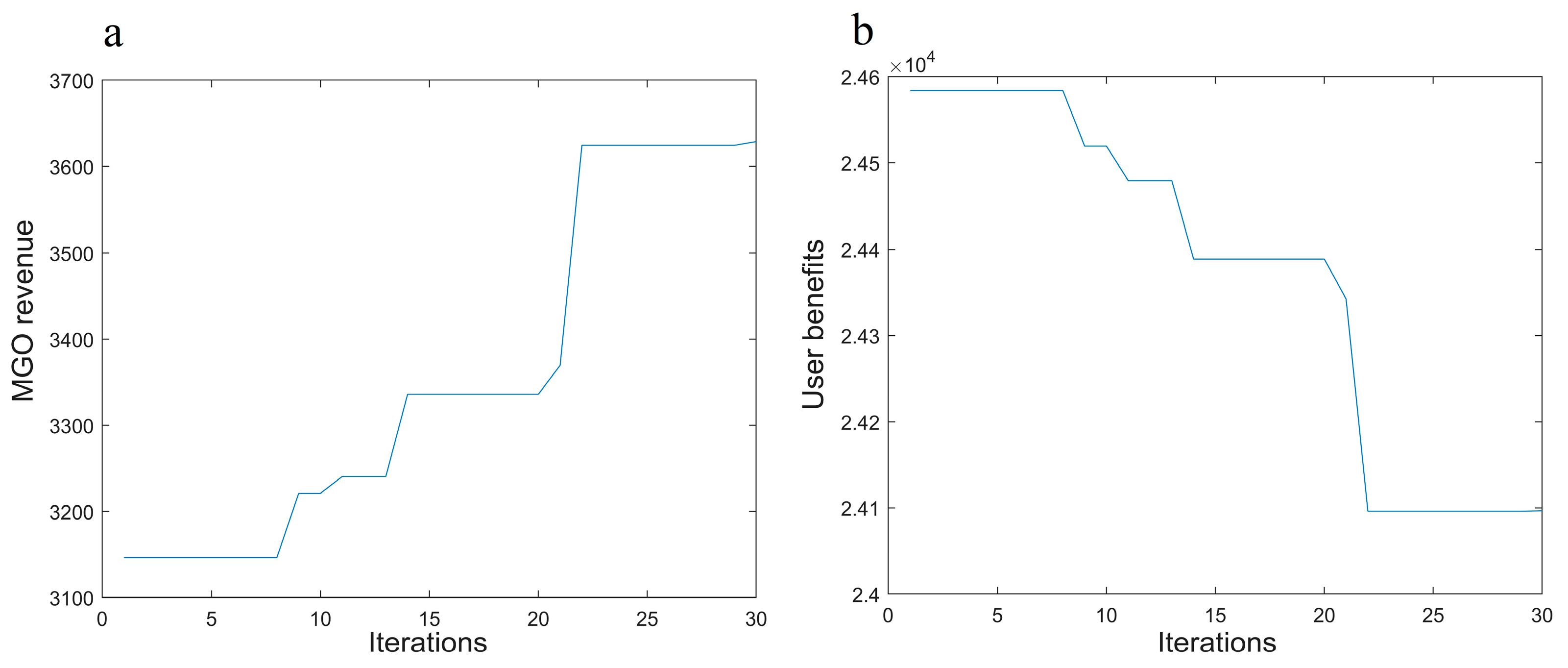
6.2. Game Equilibrium Results

The lowest comprehensive cost of the microgrid is 11,667.044709 yuan, which takes 692.513986 s. Comparing Figure 6a with Figure 6b, the game process between the microgrid and the user terminal can be analyzed. When the number of iterations is 1–8 times, the results of the game between microgrid and user do not change, and the microgrid has the lowest return and the highest user benefit. When the number of iterations is between 8 and 14, the revenue of microgrid gradually increases, and the corresponding user income gradually decreases. At a time of 15–20 iterations, both microgrid and user benefits remain the same. When the number of iterations is between 21 and 24, the revenue of microgrid increases significantly, and the corresponding user revenue decreases sharply. When the number of iterations is between 25 and 30, the microgrid revenue and user revenue once again enter a stable state.

The electricity sales plan of microgrid to users obtained by game solution is shown in Figure 7, and the load after the price-based demand response of the user is shown in Figure 8. According to Figure 7, it can be seen that the purchase price of microgrid is lower than the transaction price between microgrid and users at any time, which is the result of microgrid’s game in order to encourage users to respond and achieve the optimal overall economic dispatching level. The price signal sent by the microgrid between 12:30–18:00 and 0:00–1:00 and 2:00–5:00 at the peak time of electricity prices continues to be low, encouraging users to adjust the load during this period. According to Figure 8, it can be seen that after the introduction of price-based demand response, the user’s load curve has changed greatly, and the load has been transferred according to the real-time price adjustment given by the microgrid.

In order to verify the optimization effect of the proposed multi-group optimization method on the model, the multi-group optimization algorithm (MPGA) is compared with particle swarm optimization (PSO) and standard genetic algorithm (GA), and the results are shown in Figure 9.

As shown in

Table 3. Comparison of optimization results of different algorithms.

Algorithm	Micro-Net Total Cost/RMB	Number of Iterations
MPGA	11,667.04	31
PSO	12,306.73	74
GA	13,368.85	87

, the total cost of microgrid obtained by MPGA algorithm is 11, 667.04 yuan, which reaches convergence in 31 times. The total cost of PSO algorithm is 12, 306.7 yuan, which reaches convergence in 74 times. The total cost of GA algorithm is 13, 368.8 yuan, which reaches convergence in 87 times. It is proved that the convergence speed and one-day expenditure cost of MPGA algorithm are the best, and the optimal solution is due to other algorithms.

6.3. Optimization of Operation Results

In order to further analyze the impact of price-based demand response on the system, two comparison scenarios are set up. The carbon transaction cost, carbon emission, electricity purchase cost, gas purchase cost, and total cost of microgrid in different scenarios are shown in

Table 4. Optimization results for different scenarios.

Parameter	Consider Demand Response	Ignore Demand Response
Carbon emission/kg	4857.90	4733.93
Carbon trading cost/RMB	2303.95	2261.96
Power purchase cost/RMB	3268.39	4046.99
Gas purchase cost/RMB	6094.70	6027.04
Total cost/RMB	11,667.04	12,335.99

.

As shown in Table 3, compared with not considering demand response, in the scenario of considering demand response, the gas purchase cost has slightly increased, while the initial carbon emissions of natural gas related equipment are low, so the carbon emissions and carbon transaction costs have increased. However, based on a low-carbon model with a tiered carbon trading mechanism, the cost of electricity and total costs significantly decrease, but the increase in environmental costs is relatively small and within a reasonable range. Moreover, considering demand response can enable users to participate in the response, which is conducive to the consumption of renewable energy. The price is based on demand response and leads the user to transfer the load, so the power purchase cost is reduced. Through comprehensive calculation, the total cost of the scenario considering demand response is reduced, and the goal of economic optimal scheduling of the microgrid system is achieved.

The equipment scheduling level of the microgrid after considering the demand response is shown in Figure 10 and Figure 11, and the equipment scheduling level of the microgrid without considering the demand response is shown in Figure 12 and Figure 13.

By comparing Figure 10a and Figure 11a, it can be seen that the energy purchase period, without considering demand response, is mainly in the peak time of energy consumption, and the power purchase period in the micro grid scenario after considering demand response is mainly distributed in the peak and valley time of electricity price. By comparing the gas consumption of methanation reactions in Figure 10b, Figure 11, Figure 12b, and Figure 13, it can be seen that, considering demand response scenarios, it is 26.4% and 16.7% of the gas consumption without considering demand response scenarios, respectively. Without considering demand response, methanation reactions account for a larger proportion of the gas consumption. This is because in this scenario, the microgrid does not consider user load transfer, and purchases during the low electricity price period for the first step of hydrogen production from electricity to gas. Therefore, the hydrogen production is more than considering demand response scenarios, and as a raw material for methanation reactions and hydrogen fuel cells, it relatively reduces the purchase of natural gas during this scheduling period.

7. Conclusions

This article further rationalizes the configuration of microgrids and analyzes the respective needs of the two stakeholders, microgrids, and users. Therefore, a low-carbon economic optimization model for microgrids with a tiered carbon trading mechanism is constructed to ensure system economy while reducing carbon emissions. In addition, on this basis, a Stackelberg game model with price-based demand response, led by microgrids and followed by users, was introduced. The microgrid benefits are determined as the optimal scheduling of device operation, while the user side benefits are determined as having the highest energy efficiency, with the lowest cost. Firstly, the three elements and types of game are proposed, and the applicable game type in this chapter is Stackelberg game. Secondly, a microgrid user Stackelberg game structure was established, and the goal of the micro grid game was to achieve optimal operational economy, as well as constraints due to the consideration of increased demand response. The game goal of the user end was proposed to maximize revenue, and a satisfaction model including user electricity consumption and electricity expenditure was analyzed as a constraint to participate in the game. Once again, a Stackelberg game model was established between the microgrid and users, and it was proven that there exists an equilibrium solution to the game. Finally, an example analysis was conducted to verify the feasibility of the model. The specific conclusions are as follows:

(1)

Comparative analysis without considering demand response scenarios shows that the optimization cost of microgrid operation considering price-based demand response scenarios has decreased by 5%, which is 668.95 yuan. Among them, the power purchase cost has decreased by 23.8%, which is 778.6 yuan, the carbon emissions have increased by 17%, which is 83.96 kg, and the carbon trading cost has increased by 1.8%, which is 41.98 yuan. This proves that the introduction of demand response can improve the overall economic benefits of microgrids while slightly increasing environmental costs.

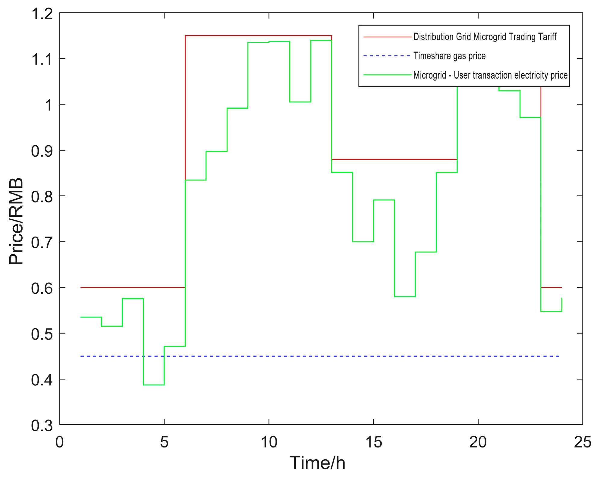
(2)

After considering demand response, the selling price of microgrids is always lower than the purchase price from the distribution network, and the price reduction rate is relatively high during the initial load valley, encouraging users to adjust their load during the time period. After the demand response, the user’s load curve underwent significant adjustments and transformations, and the corresponding load transfer was carried out according to the price signal of the microgrid, achieving the expected “peak shaving and valley filling” effect of microgrid scheduling.

(3)

In the microgrid scheduling scenario considering price-based demand response, the electricity purchase period is mainly distributed during the low and flat peak periods of tiered electricity prices. Due to the transfer of user load, the energy pressure caused by user load is reduced.

References

- BP World Energy Statistical Yearbook (2022 Edition). [EB/OL]. Available online: https://www.bp.com/en/global/corporate/energy-economics/statistical-review-of-world-energy/downloads.html (accessed on 17 June 2022).
- Speech at the General Debate of the 75th United Nations General Assembly; State Council of the People’s Republic of China: Beijing, China, 2020.
- Zhang, Y.; Zhang, N.; Dai, H. Analysis model construction and transformation path comparison of low-carbon development of China’s power system. China Power 2021, 54, 1–11. [Google Scholar]
- Zhou, N.; Fan, W.; Liu, N. Multi objective capacity optimization configuration of photovoltaic micro grid energy storage system based on demand response. Power Grid Technol. 2016, 40, 1709–1716. [Google Scholar]
- Li, X.; Geng, G.; Ji, Y. Joint optimization planning of energy storage and demand side response in active distribution network. Power Grid Technol. 2016, 40, 199–206. [Google Scholar]
- Wang, D.; Fan, M.; Jia, H. Demand Response of Home Temperature Control Load and Modeling of Energy Efficiency Power Plant Considering User Comfort Constraints. Proc. CSEE 2014, 34, 2071–2077. [Google Scholar]
- Wang, C.; Liu, M.; Lu, N. Power fluctuation smoothing method of microgrid tie line using residential temperature control load control. Proc. CSEE 2012, 32, 36–43. [Google Scholar]
- Tang, X.; Su, J.; Li, L. Optimization of economic dispatch of energy hub based on multi-energy storage microgrid. Power Capacit. React. Power Compens. 2021, 42, 182–187. [Google Scholar]
- Heiskanen, E. The Institutional Logic of Life Cycle Thinking. J. Clean. Prod. 2022, 10, 427–437. [Google Scholar] [CrossRef]
- Wu, Y.; Lv, L.; Xu, L. Comprehensive optimal configuration of multiple energy storage capacities of multi-energy microgrid considering electric/heat/gas coupling demand response. Power Syst. Prot. Control 2020, 48, 1–10. [Google Scholar]
- Zhang, X.; Wang, Z.; Lu, Z. Multi-objective load dispatch for microgrid with electric vehicles using modified gravitational search and particle swarm optimization algorithm. Appl. Energy 2022, 306, 118018. [Google Scholar] [CrossRef]
- Zheng, S.; Shahzad, M.; Asif, H.M.; Gao, J.; Muqeet, H.A. Advanced optimizer for maximum power point tracking of photovoltaic systems in smart grid: A roadmap towards clean energy technologies. Renew. Energy 2023, 206, 1326–1335. [Google Scholar] [CrossRef]
- Victoria, M.; Zhu, K.; Brown, T.; Andresen, G.B.; Greiner, M. Early decarbonisation of the European Energy System pays off. Nat. Commun. 2020, 11, 6223. [Google Scholar] [CrossRef] [PubMed]
- Chen, J.; Hu, Z.; Chen, Y. Thermoelectric optimization of integrated energy system considering stepped carbon trading mechanism and electricity to hydrogen. Electr. Power Autom. Equip. 2021, 41, 48–55. [Google Scholar]
- Saboori, H.; Hemmati, R. Considering carbon capture and storage in electricity generation expansion planning. IEEE Trans. Sustain. Energy 2016, 7, 1371–1378. [Google Scholar] [CrossRef]
- Chen, C.; Duan, S.; Cai, T.; Liu, B.; Hu, G. Optimal allocation and economic analysis of energy storage system in microgrids. IEEE Trans. Power Electron. 2011, 26, 2762–2773. [Google Scholar] [CrossRef]
- Regufe, M.J. Current Developments of Carbon Capture Storage and/or Utilization–Looking for Net-Zero Emissions Defined in the Paris Agreement. Energies 2021, 14, 2406. [Google Scholar] [CrossRef]
- Liu, Y. Research on Collaborative Optimal Scheduling of Carbon Capture and Waste Incineration Virtual Power Plants; East China Jiaotong University: Nanchang, China, 2021. [Google Scholar]
- Kirschen, D.S.; Strbac, G.; Cumperayot, P.; de Paiva Mendes, D. Factoring the Elasticity of Demand in Electricity Prices. IEEE Trans Power Syst. 2000, 15, 612–617. [Google Scholar] [CrossRef]
- Li, L.; Xue, Y.; Tian, L.; Yuan, X. Research on optimal configuration strategy of energy storage capacity in grid-connected microgrid. Prot. Control Mod. Power Syst. 2017, 2, 35. [Google Scholar] [CrossRef]
- Ma, J.; Li, L.; Wang, H.; Du, Y.; Ma, J.; Zhang, X.; Wang, Z. Carbon Capture and Storage: History and the Road Ahead. Engineering 2022, 14, 33–43. [Google Scholar] [CrossRef]
- Wei, F. Research on Integrated Energy System Planning and Operation Optimization Based on Multi-Objective Optimization and Dynamic Game Method. Bachelor’s Thesis, South China University of Technology, Guangzhou, China, 2017. [Google Scholar]
- Cheng, S.; Chen, Z.; Wang, R. Multi microgrid two-level coordinated optimal scheduling based on hybrid game. Electr. Power Autom. Equip. 2021, 41, 41–46. [Google Scholar]
- Chalkiadakis, G. Cooperative game theory: Basic concepts and computational challenges. IEEE Intell. Syst. 2012, 27, 86–90. [Google Scholar] [CrossRef]
- Makarov, Y.V.; Du, P.; Kintner-Meyer, M.; Jin, C.; Illian, H. Sizing energy storage to accommodate high penetration of variable energy resources. IEEE Trans. Sustain. 2012, 3, 34–40. [Google Scholar] [CrossRef]
- Guan, X.; Xie, S.; Chen, G. Parameter optimization method for dynamic adjustment interval of multipopulation genetic algorithm. Comput. Appl. Softw. 2022, 39, 273–282+312. [Google Scholar]
- Guan, X.; Xie, S.; Chen, G.; Qu, M. Modal parameter identification by adaptive parameter domain with multiple genetic algorithms. J. Mech. Sci. Technol. 2020, 34, 4965–4980. [Google Scholar]
- Song, W.; Dong, W.; Kang, L. Group anomaly detection based on Bayesian framework with genetic algorithm. Inf. Sci. 2020, 533, 138–149. [Google Scholar] [CrossRef]
- Sabyasachi, M.; Antonios, T. Autonomous Addition of Agents to an Existing Group Using Genetic Algorithm. Sensors 2020, 20, 6953. [Google Scholar]
- Ma, Y.; Wang, H.; Hong, F.; Yang, J.; Chen, Z.; Cui, H.; Feng, J. Modeling and optimization of combined heat and power with power-to-gas and carbon capture system in integrated energy system. Energy 2021, 236, 121392. [Google Scholar] [CrossRef]