Performance Monitoring of Wind Turbines Gearbox Utilising Artificial Neural Networks — Steps toward Successful Implementation of Predictive Maintenance Strategy

Abstract

Manufacturing and energy sectors provide vast amounts of maintenance data and information which can be used proactively for performance monitoring and prognostic analysis which lead to improve maintenance planning and scheduling activities. This leads to reduced unplanned shutdowns, maintenance costs and any fatal events that could affect the operations of the overall system. Performance and condition monitoring are among the most used strategies for prognostic and health management (PHM), in which different methods and techniques can be implemented to analyse maintenance and online data. Offshore wind turbines (WTs) are complex systems increasingly needing maintenance. This study proposes a performance monitoring system to monitor the performance of the WT power generation process by exploiting artificial neural networks (ANN) composed of different network designs and training algorithms, using simulated supervisory control and data acquisition (SCADA) data. The performance monitoring is based on different operating modes of the same type of wind turbine. The degradation models were developed based on the generated active power resulting from different degradation levels of the gearbox, which is a critical component of the WTs. The deviations of the wind power curves for all operating modes over time are monitored in terms of the resulting power residuals and are modelled using ANN with a unique network architecture. The monitoring process uses the recursive form of the cumulative summation (CUSUM) change detection algorithm to detect the state change point in which the gearbox efficiency is degraded by evaluating the power residuals predicted by the ANN model. To increase the monitoring effectiveness, a second ANN model was developed to predict the gearbox efficiency to monitor any failure that could happen once the efficiency degrades below a threshold. The results show a high degree of accuracy in power and efficiency prediction in addition to monitoring the abnormal state or deviations of the power generation process resulting from the degraded gearbox efficiency and their corresponding time slots. The developed monitoring method can be a valuable tool to provide maintenance experts with alarms and insights into the general state of the power generation process, which can be used for further maintenance decision-making.

1. Introduction

The costs of operating and maintaining wind turbines (WT) are constantly in need of reduction as WT are one of the main electricity generation technologies which has the fastest growth rate in the world [1]. Controlling the wind turbine operations by having information about the changes in wind state and the turbine position could boost the efficiency of the generated power from wind turbines [2]. The potential failures of wind turbines depend on either the instantaneous instances or the age of the components and the associated failure rates. These failures cause system outages which have significant financial consequences [3]. A wind turbine consists of several components: blades, rotor, yaw motor, tower, generator, controller, Nacelle, and gearbox [4]. The power generation capacity of wind turbines mostly depends on the gearbox that is constructed of a high-speed shaft (HSS) and low-speed shaft (LSS), which, together with the generator, makes up the drive train. Although the gearbox failure rates are typically low, they play a crucial role in wind turbine operations. Therefore, malfunctions can result in significant downtime and expensive maintenance costs [5].

Condition monitoring systems (CMS), including performance monitoring, sometimes known as “health monitoring systems,” are widely used in the literature for diagnosing faults and monitoring the health of wind turbines. CMSs include sensors, data acquisition, data processing, cabling, and other installations that provide continuous and real-time information on the monitored component condition [6,7].

In condition-based maintenance (CBM) and predictive maintenance (PdM), condition monitoring systems play a crucial role in reducing the costs of occurred failures and enhancing the functionality of any system because they are widely used as a tool for the detection of anomalies and failures by providing early warnings [8].

Supervisory control and data acquisition systems (SCADA) are one of the widely used data sources in CMS due to their cost-effectiveness and high reliability [2,9,10,11]. Many research works have used SCADA data to construct CMS of different WT components, e.g. [12,13,14,15,16,17,18,19,20,21,22]. The real-time condition of a WT component can be indicated through the measured operational data acquired from the SCADA system, such as temperature, wind speed, and the generated power, which can be analysed to derive relationships between these operational data. Subsequently, the condition of the WT can be determined using various techniques [11,23]. García et al. [24] reported several condition monitoring (CM) techniques that can be used to monitor the conditions of different WT components, such as vibration analysis, acoustic emission, ultrasonic testing, oil analysis, strain measurements, and process parameter and performance monitoring in which the relationships between different parameters, such as wind speed and the generated power can be employed to monitor the WT condition through an early detection of the associated faults or anomalies. Statistical algorithms are one of the most exploited analysis methods in CM of WTs [24], side by side with different types of machine learning (ML) techniques, such as Artificial Neural Network (ANN), Standard Classification and Regression Tree (CART), Boosting Tree Algorithm (BTA), Support Vector Machine (SVM), Random Forest (RF), Decision Tree (DT) and much more [3,14,15,25,26,27,28,29,30,31,32].

According to Hameed et al. [33], a CMS has three main characteristics; (1) Early warnings that can help avoid sudden shutdowns and improve the planning and scheduling tasks. (2) Problem identification is useful to have general insights into the health of the WT and provide the proper maintenance service at the right time. (3) Continuous monitoring of the different components of the WT and the whole system provides constant information indicating that the system is working correctly. These important characteristics help minimise shutdowns and maintenance costs, prolong component lifetimes, and ensures quality control of the different processes.

Different tools and methods can be used to monitor the process performance. Cui et al. [34] used control charts to monitor the shift in lubricant pressure by detecting the causing anomalies, while Long et al. [22] used them to monitor the performance of the generated power by analysing different power curve profiles. Similarly, Wang et al. [35] monitored the residuals of oil temperature to detect gearbox failures. Machine learning (ML) was used by Hsu et al. [25] to monitor and diagnose different faults of a WT to develop a PdM strategy to assist in planning the maintenance needs. Likewise, Wang et al. [36] used ML to monitor and detect bearing faults using SCADA data; this method was able to assess the general status of the WT with high accuracy. For the same purposes, Dao [19] developed a model to monitor the WT performance based on real SCADA data by detecting abnormal issues resulting from the changing temperature of the generator. For process monitoring and fault detection, Borchersen and Kinnaert [37] developed a fault detection and monitoring model of a WT generator cooling system. The CUSUM change detection algorithm was used to evaluate and monitor the temperature residuals.

This study proposes a performance monitoring system for WTs using ANN and CUSUM algorithm. ANN models provide accurate predictions for the generated power and the gearbox efficiency required for the monitoring process. CUSUM is utilised to develop a monitoring system to track the operational data of different modes once it deviates as the gearbox efficiency degrades. The developed monitoring system is validated and tested using simulated SCADA data of a specific WT with a nominal power of 1.25 MW working in different operational modes.

2. The Proposed Performance Monitoring System Framework

The proposed algorithm for the performance monitoring (PM) process is depicted in Figure 1.

The main steps of the proposed methodology are the following:

• Operational SCADA data Acquisition: Simulated data are collected for different operating modes of the same WT type.
• Data pre-processing: The corresponding data of the transient time are removed from the generated data sets.
• ML-ANN modelling: Two ANN models have been developed using different types of ANN training algorithms and structures to predict the gearbox efficiency of the WT in addition to the generated electrical power in different operating modes.
• After this, power residuals are calculated based on the developed ANN model, to be used in the monitoring process.
• Monitoring process: The modelled power residuals are analysed using CUSUM change detection algorithm to monitor the WT performance in different operating modes and detect any deviations or abnormal states if they exist. In addition, the gearbox efficiency prediction assists in monitoring the gearbox itself and avoids severe failure that might be caused due to the degradation of the efficiency below the manufacturer threshold.

2.1. SCADA Data and Operating Modes

The supervisory control and data acquisition (SCADA) system is a crucial component of wind turbine process performance and condition monitoring systems. SCADA systems can provide a wide range of measurements, including temperatures, wind speed, wind directions, rotor speed, pitch angle, and output power. These characteristics are frequently used to check on the health of wind farm operations. Due to its high availability, SCADA data has been used in numerous studies to estimate wind speed and power [28]. In addition to CMS sensors, the SCADA system also uses many sensors to collect data. The SCADA system monitors signals and alarms at typically ten-minute intervals [3,16].

The used datasets in this study are simulated (artificial) SCADA data using FAST-NREL simulating tool as it is described in Shaheen et al. [17]. Three operating modes with different gearbox efficiency degradation levels for the WT “DeWindD6—1250 kW” are considered in this study, knowing that the gearbox efficiency can be degraded because of a lack of lubricant, high temperature, and mechanical losses (torque losses) due to the friction between HSS and LSS. Each operating mode consisted of different percentages of gearbox efficiency. Moreover, the HSS and LSS torques are computed during the simulation based on Equations (1) and (2), taking into consideration the gearbox efficiency.

$$\mathrm{HSS}\mathrm{torque}=\frac{\mathrm{LSS}\mathrm{torque}\cdot \mathrm{efficiency}}{\mathrm{gearbox}\mathrm{ratio}}$$

(1)

$$\mathrm{LSS}\mathrm{torque}=\frac{\mathrm{HSS}\mathrm{torque}\cdot \mathrm{efficiency}}{\mathrm{gearbox}\mathrm{ratio}}$$

(2)

It is important to note that while other factors besides gearbox efficiency may affect power loss or performance degradation, this research focuses solely on monitoring a WT power generation performance by analysing the effects of the gearbox efficiency degradation on the power generation performance.

Three data features are considered with different efficiency degradation levels for three operating modes, as indicated in

Table 1. Selected input features of SCADA data.

No.	Input Feature
1	Average wind speed
2	Gearbox Efficiency%
3	Generated active power

. Each operating mode includes one thousand observations (measurements), of ten minutes average, observing average wind speed per simulation, and its associated generated active power and one efficiency level percentage e.g., 97% or 90%. Figure 2 depicts the simulated ten-minute average wind speed from 3–18 m/s. In Figure 2, a single data point represents the average wind speed of ten minutes duration.

Figure 3 depicts the main causes of the potential gearbox efficiency degradation resulting in degraded generated power.

During the data pre-processing, transient time data, outliers, missing values, and measurements below the cut-in and above the cut-off wind speed (focusing on power production areas only) of each feature measurement were removed. Figure 4 depicts the gearbox efficiency degradation levels in addition to the box plot of the simulated power for each operating mode.

The simulation tools, simulation of meteorological conditions, wind speed averaging method, and simulation control characteristics of the developed operating modes are available in detail in [17,38].

A sample scatter plot of wind speed, defined as mean wind speed and its corresponding active power (power curve form) for two different operating modes, is shown in Figure 5.

The power curve form is frequently used to show the power generated by the WT.

Table 2. The operating parameters used in the simulation process.

Cut-in Speed (m/s)	Cut-out Speed (m/s)	Rated Speed (m/s)	Rated Power (kW)	Power Law Exponent	Air Density (kg/m3)	Turbulence Intensity (%)	Mean Wind Speed of the Reference Height (m/s)	Hub Height (m)	Gearbox Efficiency (%)
2.8	23	12.5	1250	0.3	1.225	0–20	2–18	84.672	90–100

summarises the main parameters and the ideal operating conditions of DeWindD6 WT used in the simulation process of the nominal power curve and the other different operating modes.

Complete technical characteristics of the DeWindD6 WT are available in [39].

The power curve of any wind turbine in real applications is dynamic because of the constantly changing working conditions, such as the weather, temperature, wind speed, air density, system controls, and humidity. As a result, the variation in wind speed and direction affects different parameters, such as rotor speed (the desired speed in RPM), pitch angle and the generated power [40]. The wind speed and the desired rotor speed of the WT based on its power curve determine the best pitch angle of the blades; the optimum wind direction gives the maximum generated power when it is perpendicular to the blades. Overall, wind speed variations lead to a change in the generated power.

2.2. Artificial Neural Network Prediction Models

Over the past twenty years, artificial neural networks (ANN) have increasingly become one of the essential machine learning (ML) prediction techniques [41]. ANN algorithms have demonstrated their ability to operate with high accuracy and minimal error, demonstrating their suitability for prediction in a variety of applications [42,43,44,45,46,47].

The purpose of neural networks is to emulate the functions of real biological brain networks. The neuron is the fundamental component of neural networks, and, depending on the tasks it performs, it can alter in size and shape. The ANN is made up of node layers, including an input layer, an output layer, and one or more hidden layers as seen in Figure 6. The complete procedure of ANN training can be described using the inputs, weights, summation function, and activation function [48,49]. Each node has a threshold and weight, and they are all connected. When a node’s value crosses the threshold, it activates, and the data is sent through it. The inputs are the data gathered from the primary sources offered. The weights control how the inputs influence the neuron and are constantly adjusted to improve the input-output relationship. The weighted summation function determines what the net inputs are. The activation (transfer) function accepts the net input from the summation function and uses it to calculate the neuron’s output. This is possible because the activation functions are either linear or non-linear algebraic equations that enable the network to store the various relationships between the inputs and outputs during training. Lastly, the outputs take the results provided by the activation function and accept them to be delivered for additional processing outside the network.

The multi-layer perceptron (MLP), the most popular ANN architecture, can be employed with a variety of training algorithms, including gradient descent (GD), Levenberg-Marquardt (LM), and error backpropagation (EBP) with conventional forward-backward computing [41,50,51].

On the other hand, to enhance the training process and allow the ANN to train and model complicated structures like fully connected networks (FCN) and arbitrarily connected networks (ACN), alternative network designs in combination with the neuron-by-neuron training algorithm (NBN) were developed. This may be used to train and model systems with complicated structures and handle an infinite number of input patterns [49,52,53,54,55]. It can also be used to represent arbitrary connections in networks.

In this study, the Matlab software tool was mainly used for SCADA data simulation and analysis in addition to various statistical analysis software for data pre-processing and data visualisation. The software used for training was the “NBN Trainer 2.08” that was built using the C++ programming language by Yu et al. [56].

Initial weights for the neural networks are random weights between −1 and 1. Hyperbolic tangent (tanh) is the activation function utilised for hidden layers (employed by the neurons) and the output layer as well, taking into consideration the fact that, in this case, neurons can produce positive or negative outputs. [55]. Neuron $j$ output is described in Equation (3).

$${\mathrm{Out}}_j=\tan \mathrm{h}\left(\mathrm{gain}\times ne{t}_j\right)+\mathrm{der}\times ne{t}_j$$

(3)

where $ne{t}_j$ is the sum of the weighted inputs to neuron j, and ${\mathrm{Out}}_j$ is the output of neuron j.

The “gain” and “der” are parameters of the activation functions. The parameter “der” is introduced to adjust the slope of the activation function where the slope is approaching zero [56].

The degradation measurements, which should be the output of the training, are normalised using the min-max normalisation process using Equation (4).

$$x^{\prime }=\frac{x-min\left(x\right)}{max\left(x\right)-min\left(x\right)}$$

(4)

where $x^{\prime }$ is the normalised value, and $x$ is the value to be normalised; $min\left(x\right)$ and $max\left(x\right)$ are the maximum and minimum values of the range from which $x^{\prime }$ has been normalised. It is worth mentioning that data normalisation in ANN training helps models to converge faster with higher learning rates.

When the slope of the activation function gets close to zero, the parameter “der” is provided to adjust it [56]. “Gain” and “der” were set to 0.50 and 0.01, respectively.

In this research, two ANN models were developed to predict the generated power and the gearbox efficiency of different operating modes of the WT separately. The more accurate model of the two was selected based on the least error; then, it was used to calculate the power residuals needed for the performance monitoring process.

2.2.1. Power Prediction ANN Models

Two ANN models were developed to predict the power, ANN-MLP, and ANN-NBN. The datasets of operating modes 1 and 3 were used to train and test the developed models with 80%–20% training and testing splitting ratio. While the dataset of operating mode 2 was used to validate the developed models.

Table 3. Summary of the ANN models developed for the prediction of the generated power and gearbox efficiency.

ANN Model	Model I	Model II
Variable’s normalisation	Min-max normalisation
Architecture	MLP 2-2-1	FCN/ACN
No. neurons	H3	3
Hidden layers activation function	Hyperbolic tangent (tanh)
Outputs activation function	Hyperbolic tangent (tanh)
Training algorithm/computations method	LM—forward-backward	NBN—forward-backward
No. patterns/training (80%)	1600
No. patterns/test (20%)	400
Error function	Root mean squared error (RMSE)

presents a summary of the developed two ANN models.

The predicted power was modelled in terms of the wind speed and gearbox efficiency using the ANN architectures depicted in Figure 6.

2.2.2. ANN Models for Gearbox Efficiency Prediction

The same architecture of the two models explained above was also used to predict the gearbox efficiency utilising the datasets of operating modes 1 and 3 for testing and training, while the dataset of operating model 2 was used for validation. Table 3 presents a summary of these ANN models.

The predicted gearbox efficiencies were modelled in terms of wind speed and power using the ANN architectures depicted in Figure 7.

It’s worth mentioning that the developed prediction models are solely based on the simulated datasets of the three operating modes of the WT type “DeWindD6 1250 kW” and can be generalised to other types of WTs in future works.

2.3. Model Evaluation

The developed models were evaluated in terms of their prediction accuracy using the statistical performance measure root mean squared error (RMSE), as Equation (5).

$$\mathrm{RMSE}=\sqrt{{{\displaystyle \sum }}_{i=1}^n\frac{{\left({\widehat{y}}_i-y_i\right)}^2}{n}}$$

(5)

where $n$ is the number of patterns, ${\widehat{y}}_i$ is the predicted value, and $y_i$ is the target (measured) value.

2.4. Power Residuals

The term “power residual” refers to the difference between the measured power and the predicted power based on the selected ANN model among the developed ones, as Equation (6).

$$\mathrm{Power}\mathrm{residual}\left({\mathrm{r}}_{\left(\mathrm{i}\right)}\right)=\mathrm{Power}\_\mathrm{measured}-\mathrm{Power}\_\mathrm{predicted}$$

(6)

3. Results and Discussion

3.1. Evaluation, Selection, and Validation of ANN Prediction Models

Table 4. Validation metrics using RMSE to evaluate the developed prediction models.

	Power Prediction Models		Efficiency Prediction Model
ANN Model	Model I	Model II	Model I	Model II
Training RMSE—Normalised	0.0222	0.0191	0.0388	0.0359
Testing RMSE—Normalised	0.0219	0.0195	0.0396	0.0367
Validation RMSE—Normalised	0.0212	0.0198	0.0192	0.0230
Average RMSE -Normalised	0.0217	0.0194	0.0325	0.0318

shows the validation metrics based on the performance measure RMSE used for checking the prediction accuracy of the developed ANN models.

It can be seen that all models have a relatively small RMSE; training, testing, and validation RMSE values are close to each other. The least RMSE means better prediction performance. Thus, the best RMSE value was achieved by model II (ANN-NBN) with slightly lower RMSE values than models I. Model II of power predictions was selected then to calculate the power residuals and monitor the performance of the WT power generation process.

It is worth mentioning that the dataset of operating mode 2 was used for further validation of model II for both the prediction of power and gearbox efficiency. It is known that for the simulation of this dataset, the efficiency was set to 97%. During validation, the efficiency of this dataset was predicted at 96.4%, which can be considered as a high prediction accuracy.

3.2. Prediction Analytical Equations

To provide a practical way to predict the output power of WT with different gearbox efficiency levels, in addition to predicting the gearbox efficiency itself, two analytical equations, Equations (9) and (10), were extracted from the ANN models based on their weights and biases.

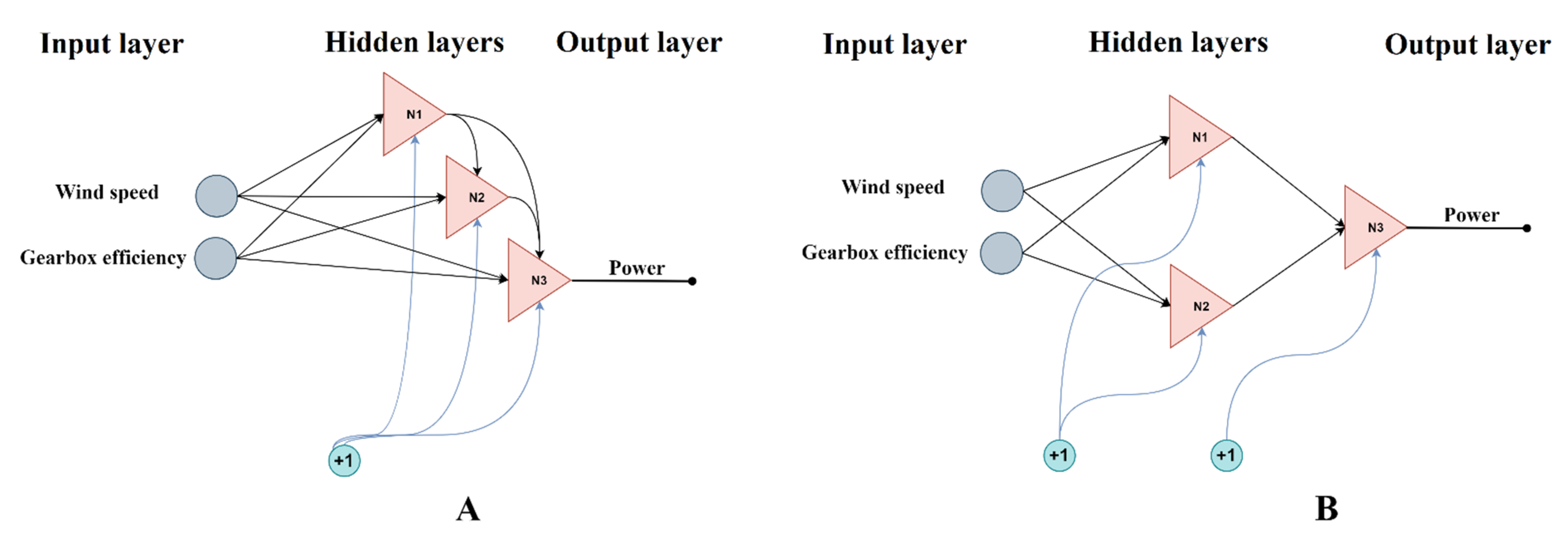
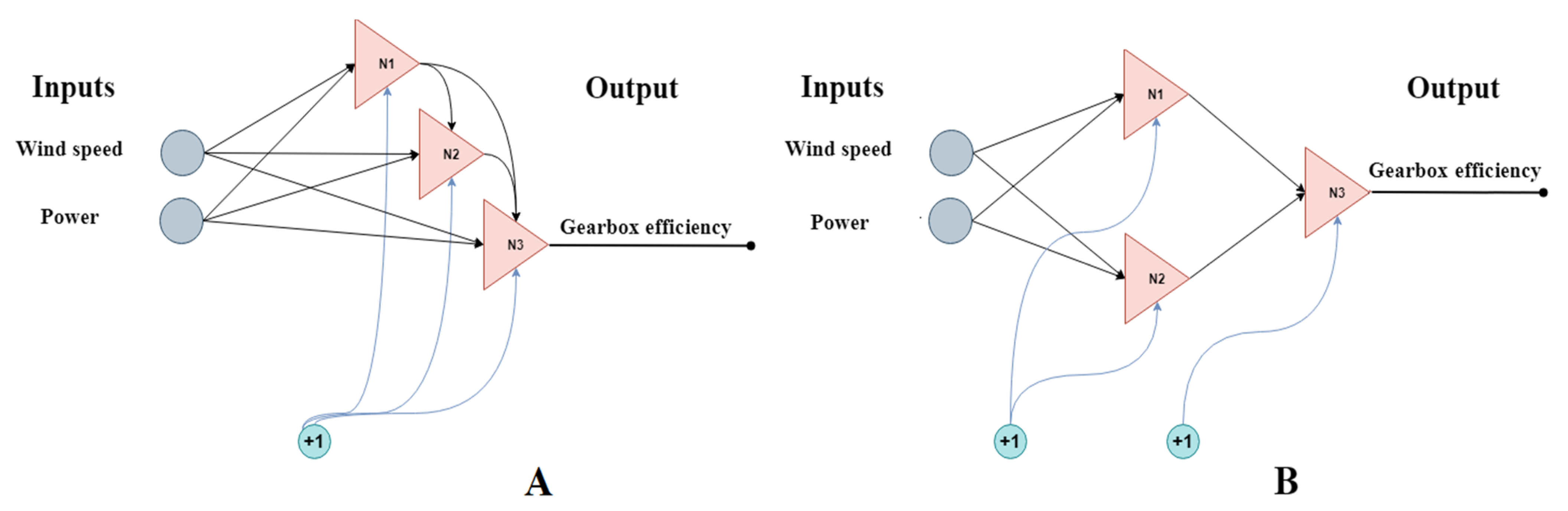
Regarding the prediction models, there were 12 estimated weights for each: input weights (IW) between the inputs and hidden layers and layer weights (LW) between the hidden layers and the output. Two inputs and one output are included in each model. The biases are b1 for the input layers and b2 for the output layer. The weights are taken from the best-trained ANN models based on the lowest RMSE (Model II for both power and gearbox efficiency prediction).

Referring to Equation (3), substituting the values of “der” and “gain” the activation function $f\left(x\right)$ can be written as:

$$\begin{array}{l}f\left(x\right)=\tanh \left(0.5x\right)+0.01x \\ f\left(x\right)=\frac{e^{0.5x}-e^{-0.5x}}{e^{0.5x}+e^{-0.5x}}+0.01x\end{array}$$

(7)

then,

$$\mathrm{Power}\mathrm{prediction}=b_2+LW·\tan \mathrm{h}\left(b_1+IW·x\right)$$

(8)

$${\mathrm{Power}\mathrm{prediction}}_i^{}=3.371+1.307·\frac{e^{\left(1+IW·0.5x\right)}-e^{-\left(1+IW·0.5x\right)}}{e^{\left(1+IW·0.5x\right)}+e^{-\left(1+IW·0.5x\right)}}+0.01\left(b1+IW·x\right)$$

(9)

where $x$ is the inputs matrix.

Table 5. Weights and biases of the best-trained ANN power prediction model.

b1	b2	IW			LW
17.09214	-	−18.95625	−6.37007	-	-
−0.36432		0.99391	−0.33618	−2.33843	-
-	3.37135	1.53391	0.15928	−2.73824	1.30765

provides the estimated values of (b1), (b2), (IW), and (LW) from the best-trained ANN model used for power prediction. Similarly,

Table 6. Weights and biases of the best-trained ANN gearbox efficiency prediction model.

b1	b2	IW			LW
2.37085	-	−6.87395	−9.08612	-	-
−10.38677	-	0.12185	5.35551	−5.03385	-
-	−562.47041	26.5025	705.80450	147.0163	−493.26603

provides the same estimates from the best-trained ANN model developed for gearbox efficiency.

$${\mathrm{Gearbox}\mathrm{efficiency}\mathrm{prediction}}_i^{}=-562.47-493.266·\frac{e^{\left(1+IW·0.5x\right)}-e^{-\left(1+IW·0.5x\right)}}{e^{\left(1+IW·0.5x\right)}+e^{-\left(1+IW·0.5x\right)}}+0.01\left(b1+IW·x\right)$$

(10)

3.3. Importance Analysis

The influence of each input variable of the developed best performance ANN models for both power and gearbox efficiency prediction was analysed using the predictors’ importance analysis to order the variable predictors according to their respective “importance”.

Table 7. Importance analysis for all operating modes in terms of wind speed.

Power Predictions ANN Model II				Gearbox Efficiency Predictions ANN Model II
Feature	Variable Rank %	Importance	Order	Variable Rank %	Importance	Order
Wind speed	97	0.971	1	90	0.9013	2
Power	-			100	1	1
Gearbox efficiency	3	0.029	2	-

and Figure 8 show that the most significant input feature is wind speed for the power prediction model, with around 97%, while the gearbox efficiency has the lowest effect, with only 3%. Similarly, both power and wind speed are influential input features with respect to gearbox efficiency prediction, with 90% and 100%, respectively.

In practice, the gearbox efficiency is also an influential input in terms of power prediction; the decreased level of gearbox efficiency causes a decrement in the generated power in a manner that the power curve is shifted downwards. In this study, the importance of efficiency resulted in a small portion compared to the wind speed due to the limited exploited efficiency degradation levels (three operating modes).

3.4. Power Residuals Calculation

The power residuals based on the ANN model II predictions were calculated using Equation (6).

The statistical summary of the power residuals based on the predictions by the ANN model II used in the monitoring process is presented in

Table 8. Statistical summary of the calculated power residuals of each operating mode.

Operating Mode	Mean	Standard Deviation	Variance	Range	Min	Max
1	1.078	22.498	506.164	144.217	−59.175	85.043
2	−2.403	23.390	547.085	146.479	−70.241	76.239
3	−2.110	22.881	523.526	147.682	−77.040	70.642

.

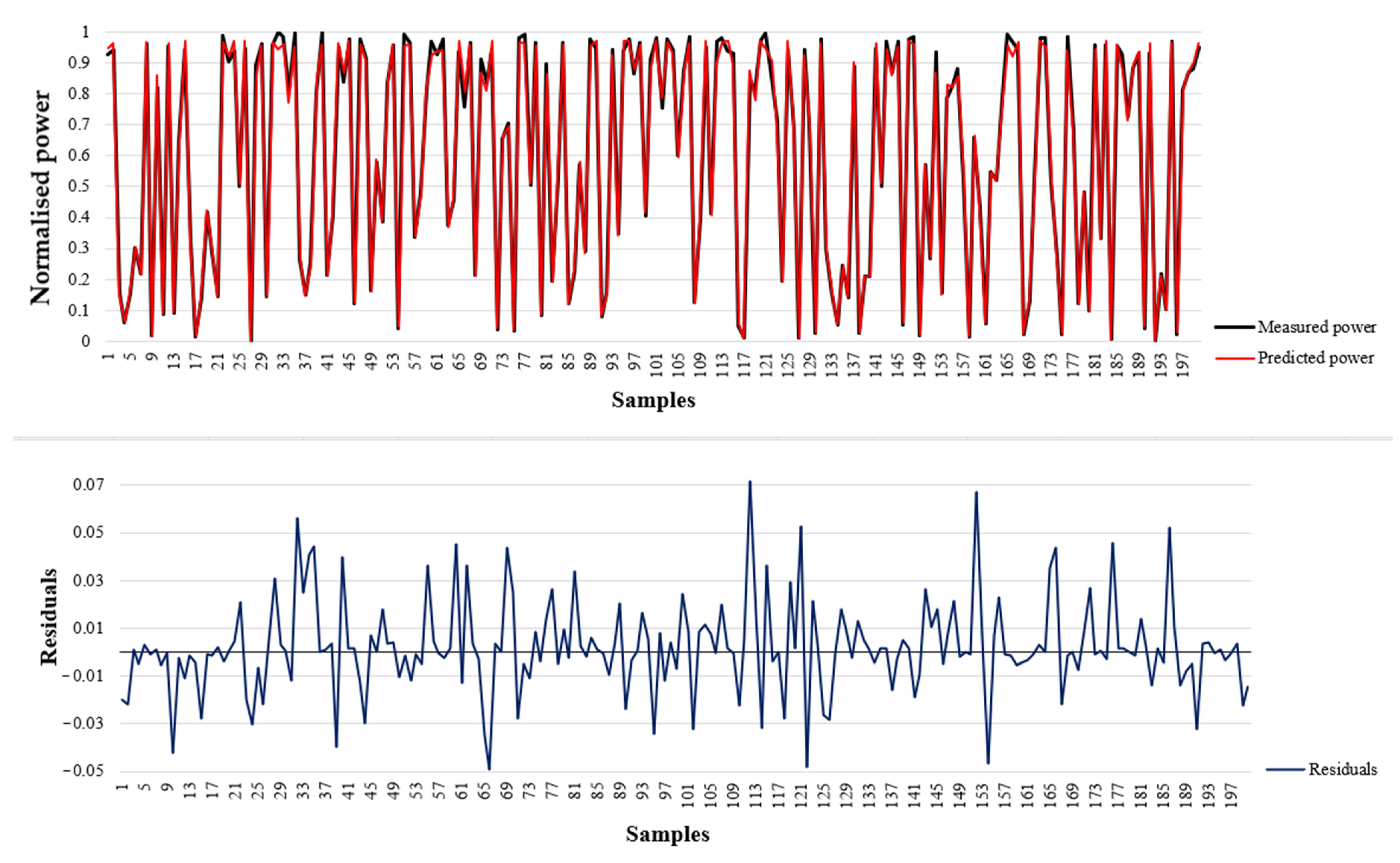
A sample of the normalised measured and predicted power and their calculated residuals are presented in Figure 9.

It can be noticed from Figure 9 and Table 4 that the prediction error (RMSE) is relatively small for both power prediction models; the training and testing RMSEs are relatively close to each other.

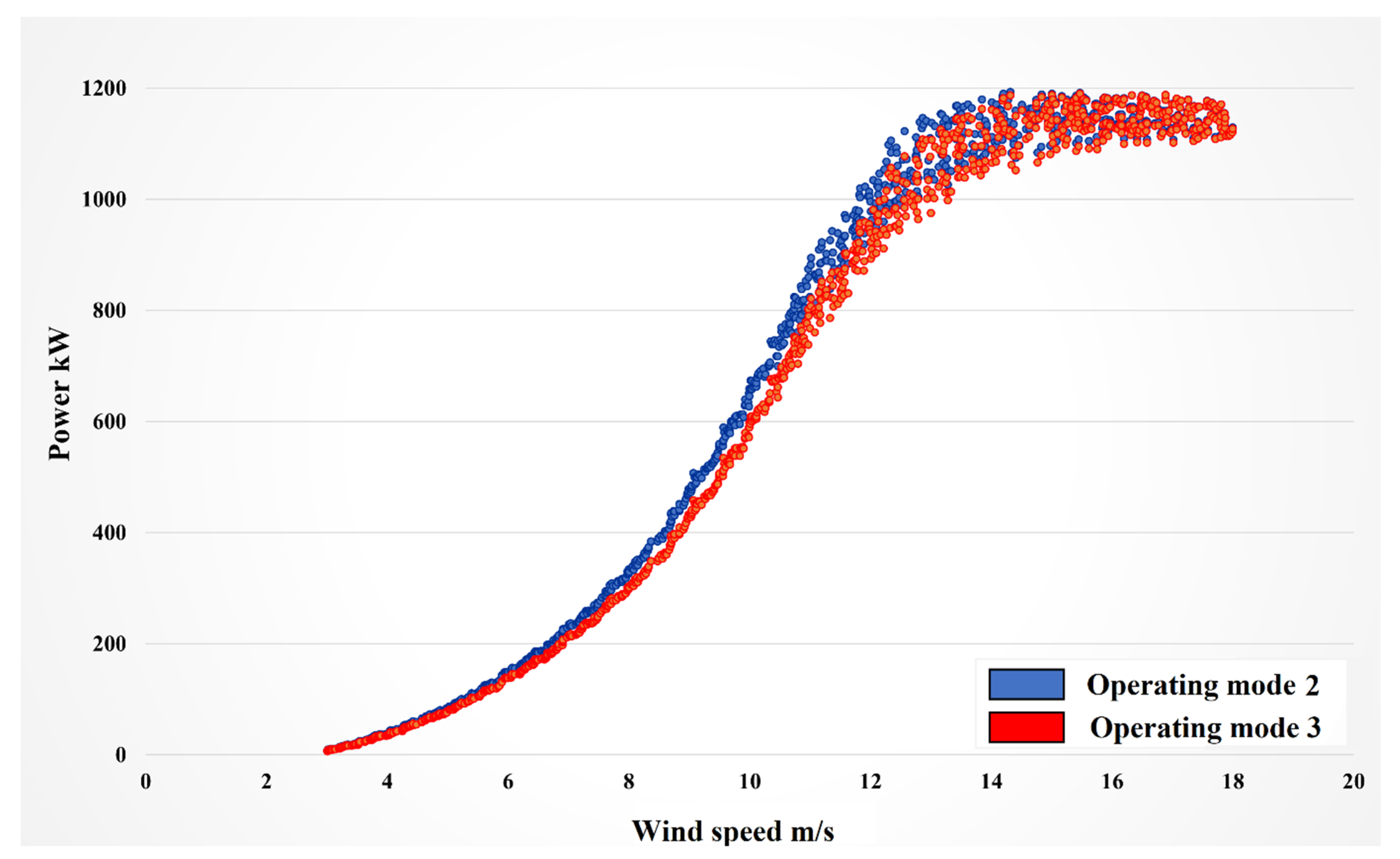
To sum up, the validation of the developed prediction models was based on two measures: the performance metrics of the models (RMSE) and the prediction accuracy, using the dataset of operating mode 3, which showed reasonable and accurate results as discussed before.

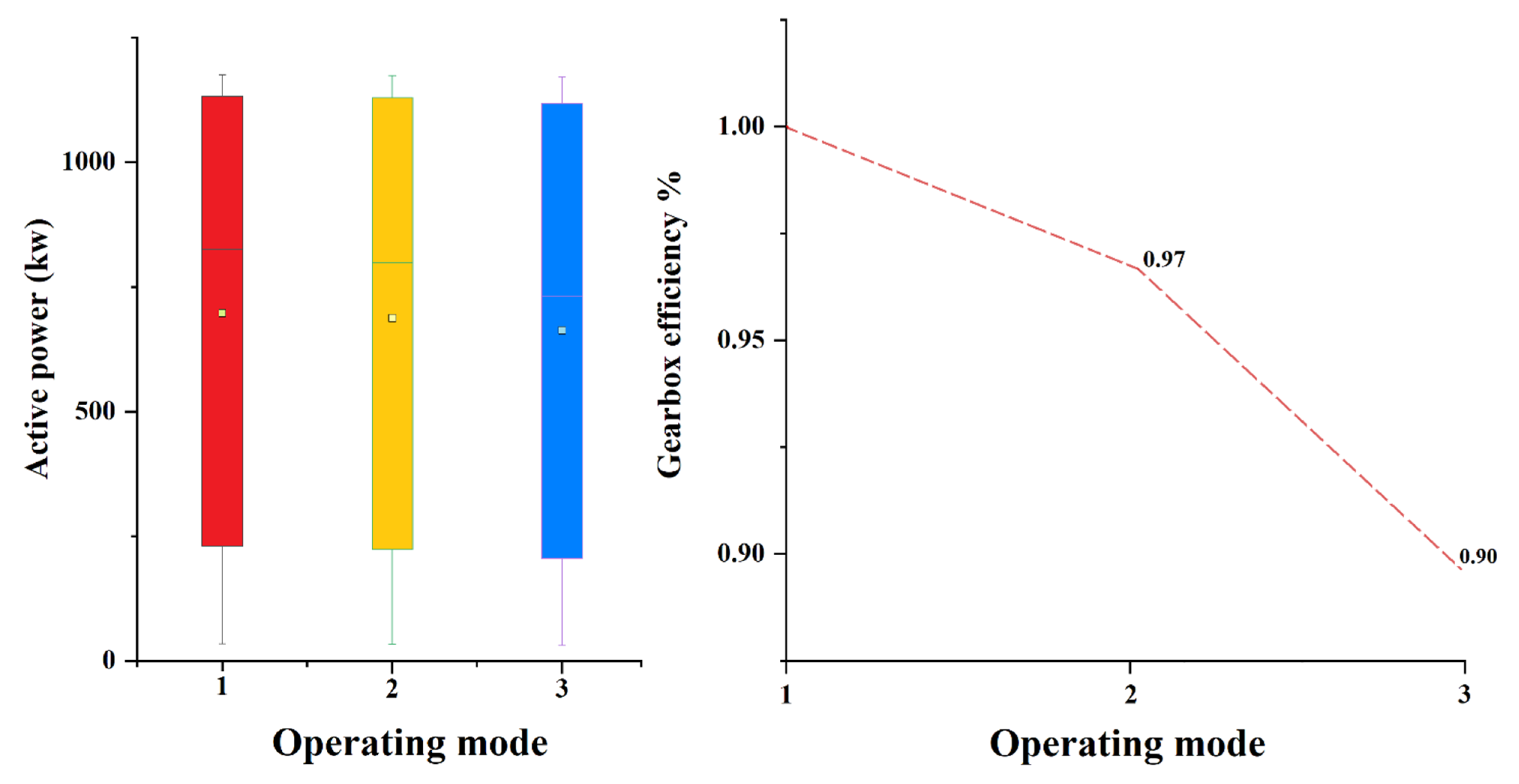
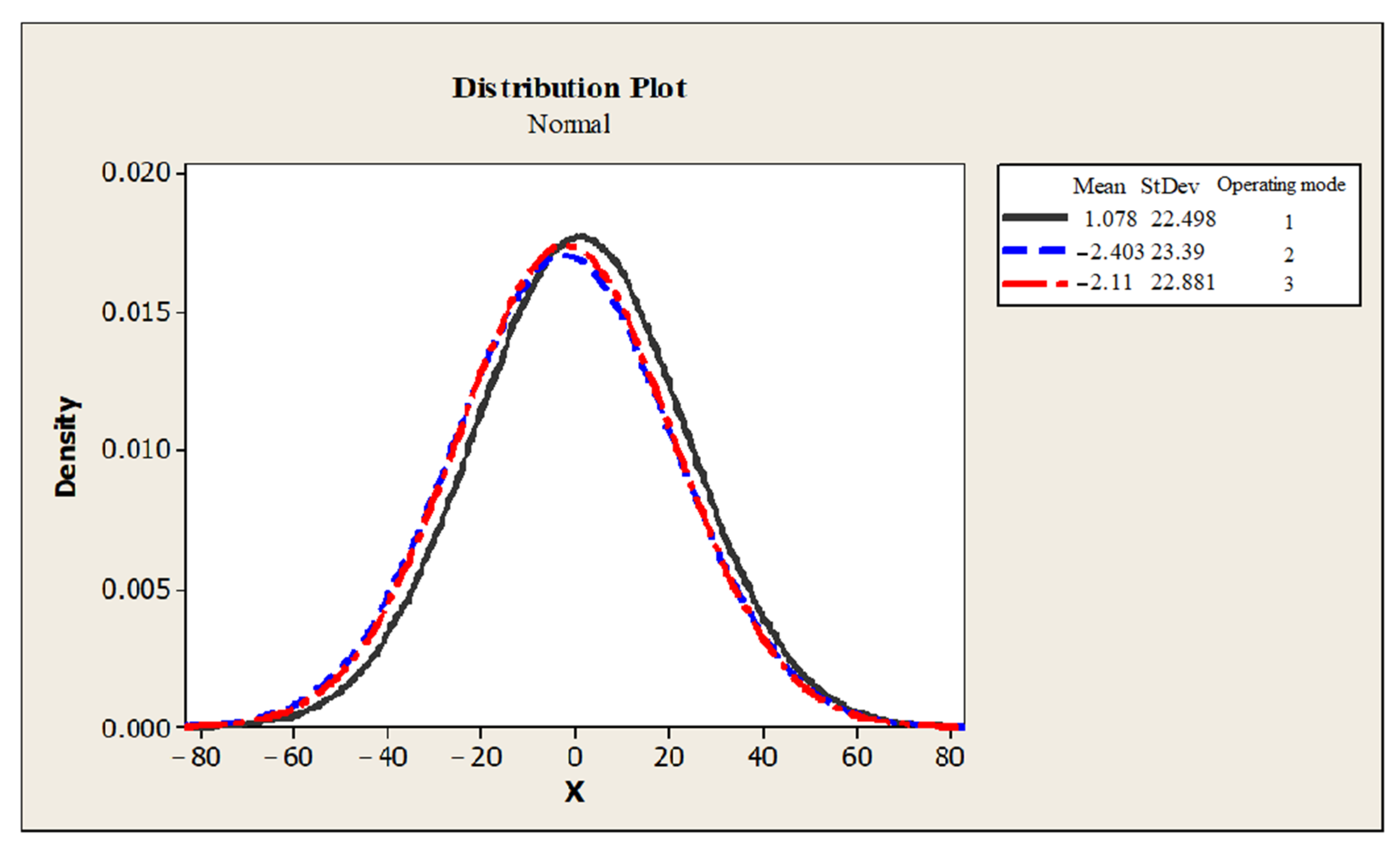
Figure 10 shows the probability plot of power residuals for the three operating modes. From Table 8 and Figure 9, it can be observed that the values of the power residuals for the operating modes 1–3 resulting from the ANN model predictions have significant variations. Thus, the mean of each operating mode has indicated that all residuals are shifted toward the negative side due to the increased degradation in the gearbox efficiency.

Figure 10 shows the power residuals probability density function (PDF) predicted by ANN model II for all operating modes, from which we can observe that operational modes 2 and 3 have a small negative shift in their means due to the degradation in both gearbox efficiency and the affected power generation.

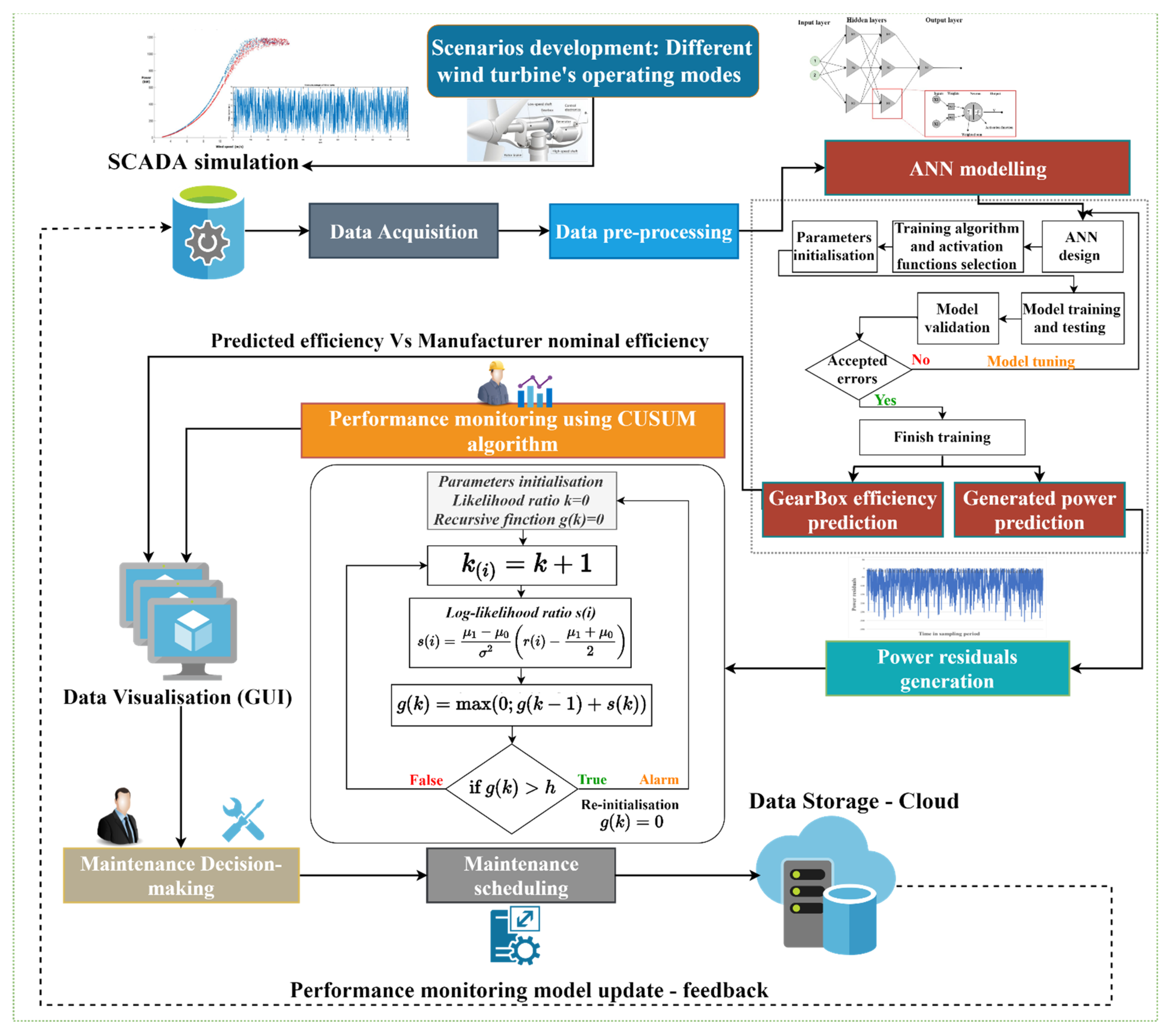
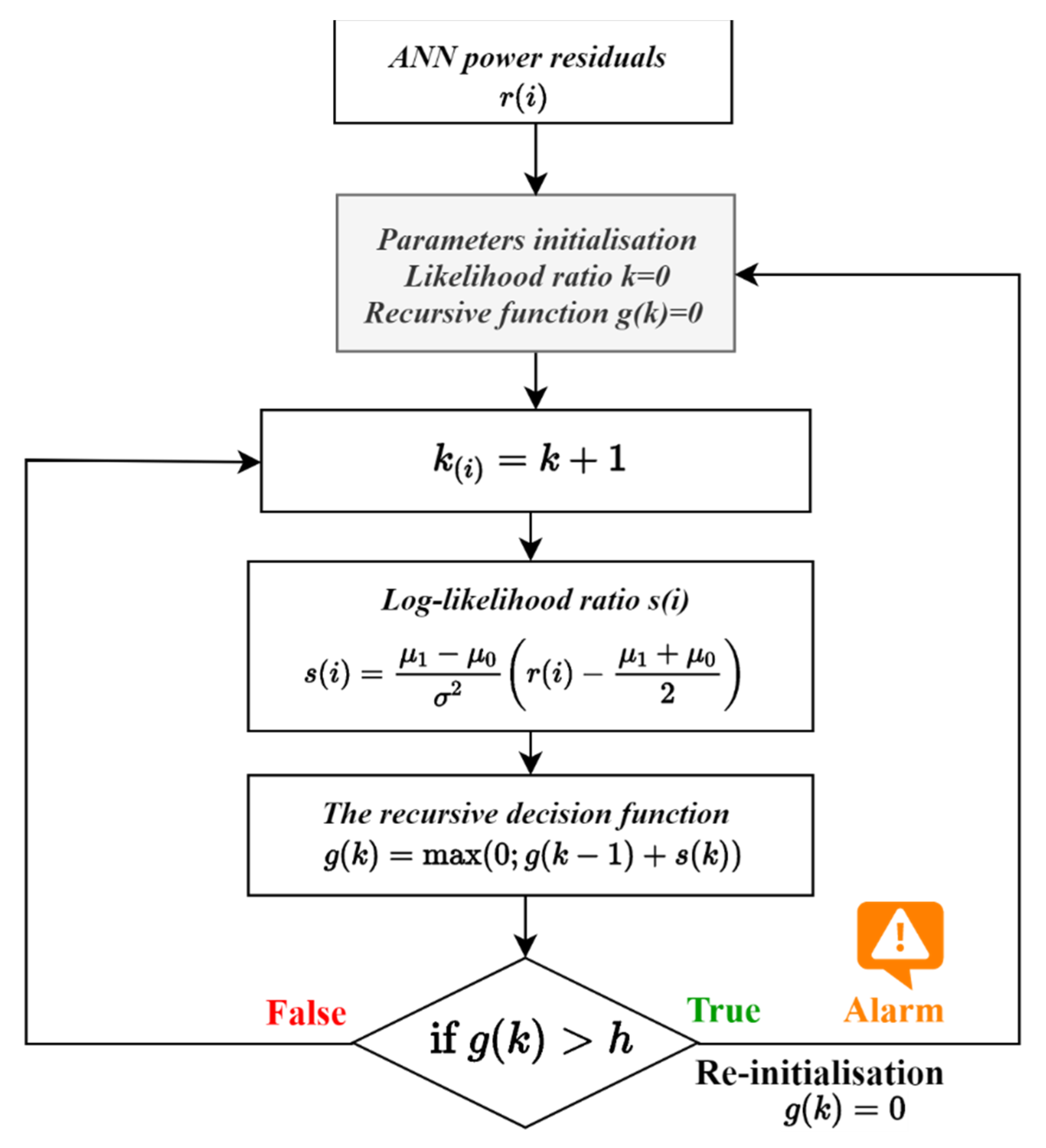
3.5. Performance Monitoring Using CUSUM Change Detection Algorithm

The cumulative summation (CUSUM) algorithm is usually utilised for state change detection and performance monitoring. It is known for its robustness in detecting small changes in the mean of the time series which is stationary between two changepoints.

The ANN-NBN model II of the power prediction, as shown in Table 4, has a small error. Hence, the power prediction model II and its related power curve can be used as a baseline for the monitoring process. Once the WT is operating as the baseline (normal state), the model can provide accurate predictions of the power output along with minor power residuals between the measured and the predicted power. When the WT has abnormal operating conditions, the output variables deviate from the baseline model, and then the model produces increasingly shifted predicted power residuals. Using the ANN model II as a baseline, the performance of each operating mode in terms of the produced power is monitored. The monitoring process aims at detecting any abnormal state change related to the power residuals. The CUSUM change detection algorithm test is performed for that purpose as shown in Figure 11.

The main goal of the CUSUM test is to compare two hypotheses ${\mathscr{H}}_0\mathrm{and}{\mathscr{H}}_1$, which represent the normal and abnormal states of the different operating modes, respectively, to see which one best fits the given datasets.

A scalar set of the ANN predicted power residuals $r\left(i\right)=\left\{r\left(1\right),r\left(2\right)\dots \dots r\left(k\right)\right\}$ is used as an input. Assuming that the power residuals have a Gaussian (normal) distribution, then the hypotheses are as follows:

$$\begin{array}{l}{\mathscr{H}}_0:r\left(i\right)~ \mathcal{N}\left({\mu }_0,{\sigma }^2\right)fori=\left(1,\dots ,k\right)\\ {\mathscr{H}}_1:r\left(i\right)~ \mathcal{N}\left({\mu }_0,{\sigma }^2\right)fori=\left(1,\dots ,k_0\right),r\left(i\right)~ \mathcal{N}\left({\mu }_1,{\sigma }^2\right)fori=\left(k_0,\dots ,k\right)\end{array}$$

where:

$k_0$ is the unknown change time;

${\mu }_0$ and ${\mu }_1$ are the means of the ANN power residuals before and after the potential change, respectively;

$k$ is the number of measuring points.

The corresponding log-likelihood ratio $s\left(i\right)$ for detecting a change in the mean of the ANN power residuals from ${\mu }_0$ (normal state—operating mode 1) and ${\mu }_1$ (abnormal state—operating mode 2 and 3) can be obtained with Equation (11).

$$s\left(i\right)=\frac{{\mu }_1-{\mu }_0}{{\sigma }^2}\left(r\left(i\right)-\frac{{\mu }_1+{\mu }_0}{2}\right)$$

(11)

The recursive form of the CUSUM algorithm is an efficient method for performing the CUSUM test. The recursive form of the decision function is calculated as Equation (12).

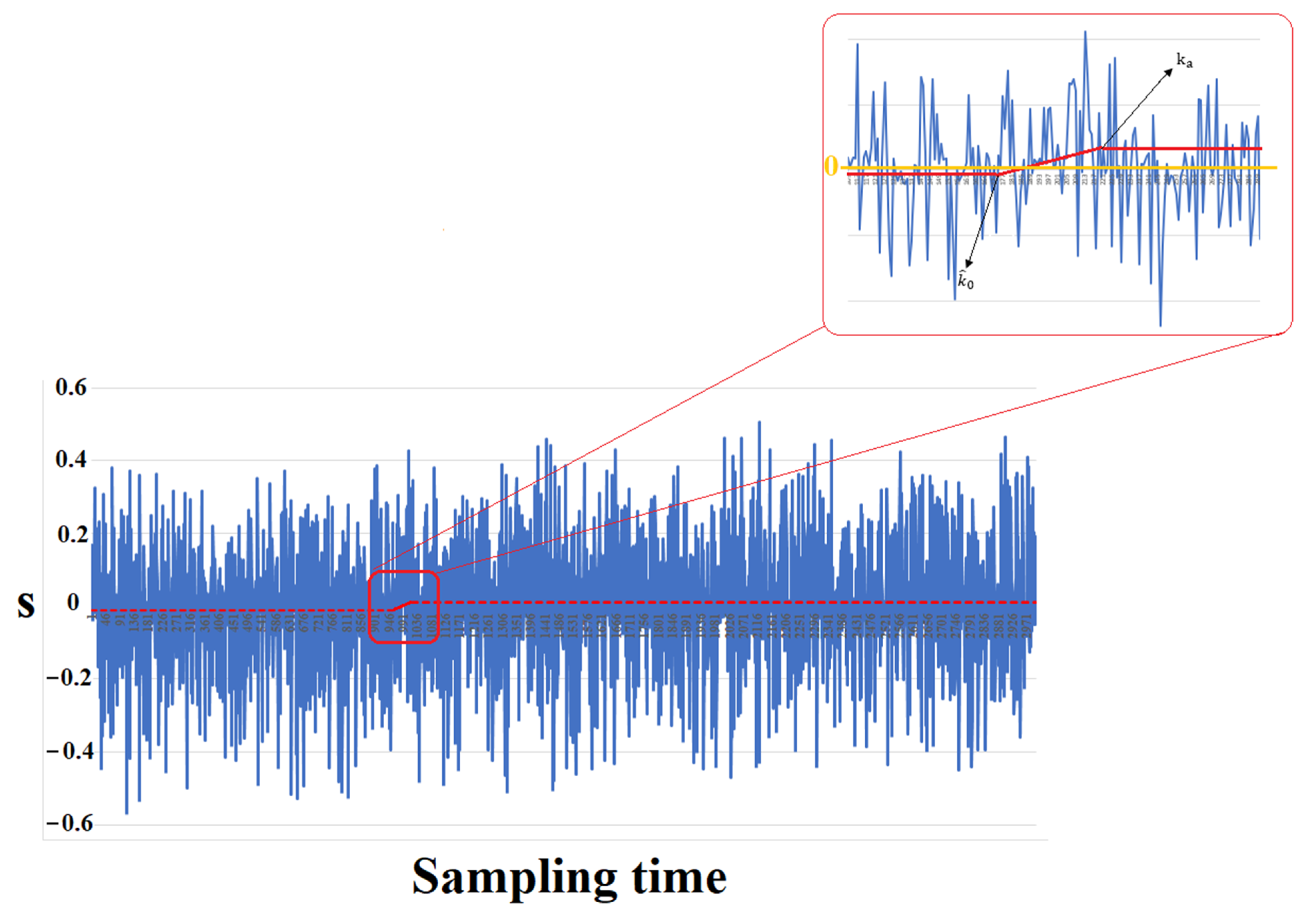
The log-likelihood ratio $s\left(i\right)$ has a negative value before the change resulting from the degradation in the gearbox efficiency, and then it has a positive drift after the change along with the change occurrence time ${\hat{\mathrm{k}}}_0$ and the stopping time ${\mathrm{k}}_{\mathrm{a}}$, as can be seen in Figure 12.

$$g\left(k\right)=max\left(0;g\left(k-1\right)+s\left(k\right)\right)$$

(12)

The alarm function is presented in Equation (13).

$$d\left(k\right)=\{\begin{array}{c}1, if g\left(k\right)>h\\ 0, otherwise\end{array}$$

(13)

A user-defined threshold $h$ is used to make a reasonable balance between a quick-change detection and a low false alarm rate; $h$ is always positive; only the contributions to the cumulative sum that add up to a positive number must be considered to determine the decision function [57].

To avoid or reduce the false alarms and missed change detections caused by the parameter variations, the $h$ must consider the maximum magnitudes of residuals under the normal state of the operating mode, and then the threshold can be calculated as Equation (14).

$$h=1.5\times \{maxg\left(k\right):k<k_a\}$$

(14)

The stopping time ${\mathrm{k}}_{\mathrm{a}}$, which can be called alarm time as well, is the time instant at which $g\left(k\right)$ crosses the $h$.

$$k_a=\min \left\{k:g\left(k\right)\ge h\right\}$$

(15)

The change occurrence time $k_0$ can be estimated as the time instant ${\widehat{k}}_0$ at which $s\left(k\right)$ changes from negative to positive slope as indicated by Equation (16).

$${\widehat{k}}_0=k_a-N\left(k_a\right)$$

(16)

$N\left(k\right)$ is the number of successive observations in which the decision function remains positive, as expressed in Equation (17).

$$N\left(k\right)=N\left(k-1\right)1_{\{\mathrm{g}\left(\mathrm{k}-1\right)>0\}}+1$$

(17)

where $1_{\{\mathrm{g}\left(\mathrm{k}-1\right)>0\}}$ is the indicator of event $\mathrm{g}\left(\mathrm{k}-1\right)>0$, namely, $1_{\{\mathrm{g}\left(\mathrm{k}-1\right)>0\}}$= 1 when $\mathrm{g}\left(\mathrm{k}-1\right)>0$ is true, otherwise $1_{\{\mathrm{g}\left(\mathrm{k}-1\right)>0\}}$ = 0.

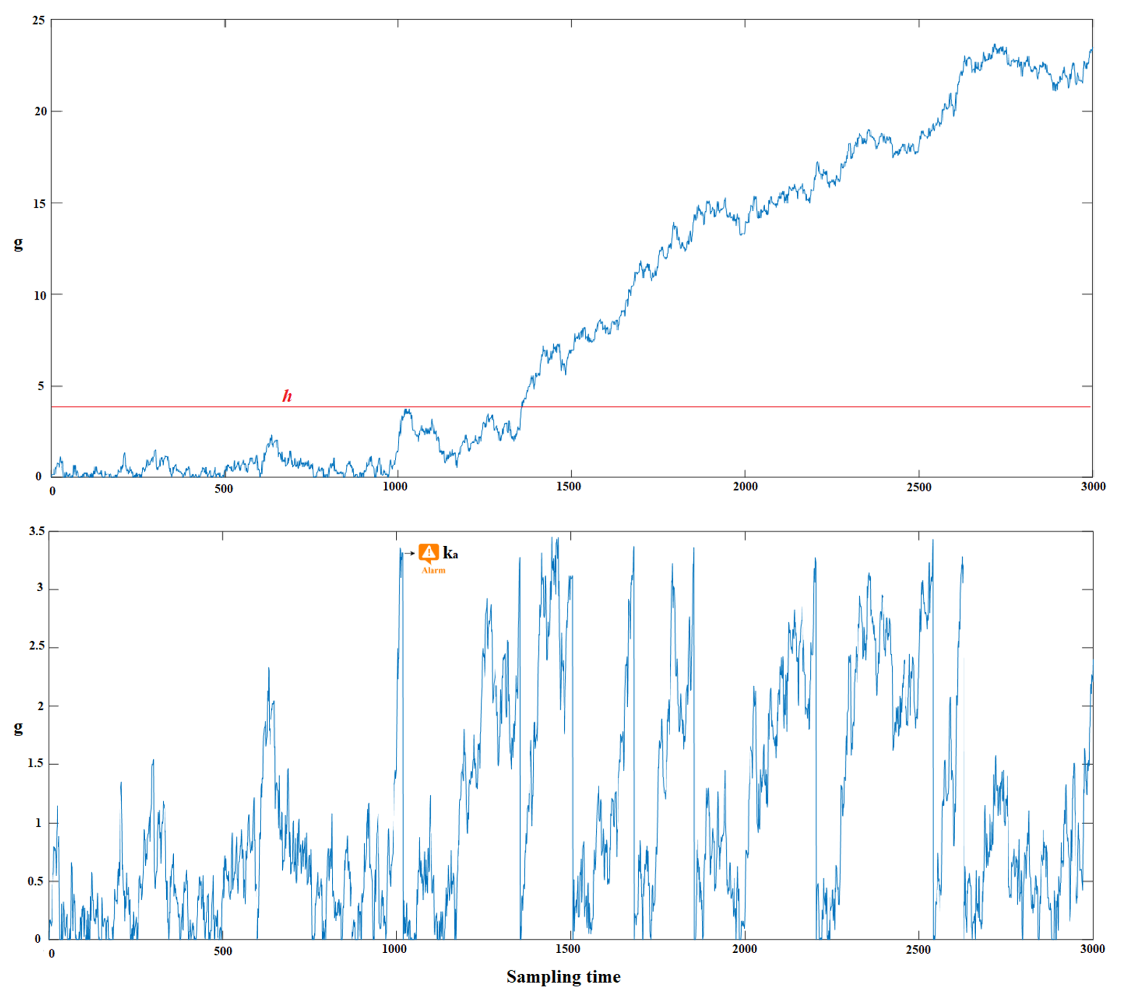
Figure 13 shows the recursive CUSUM decision function of the ANN power residuals for the three operating modes, in which the first operating mode is considered normal and the others as abnormal states in terms of the degraded gearbox efficiency. The upper chart presents the recursive CUSUM without re-initialisation, where $h=3.459$. While the lower chart presents the recursive CUSUM with re-initialisation once $h$ is crossed ($g\left(k\right)>h$). The stopping time (alarm) $k_a$= 1018 is also shown there.

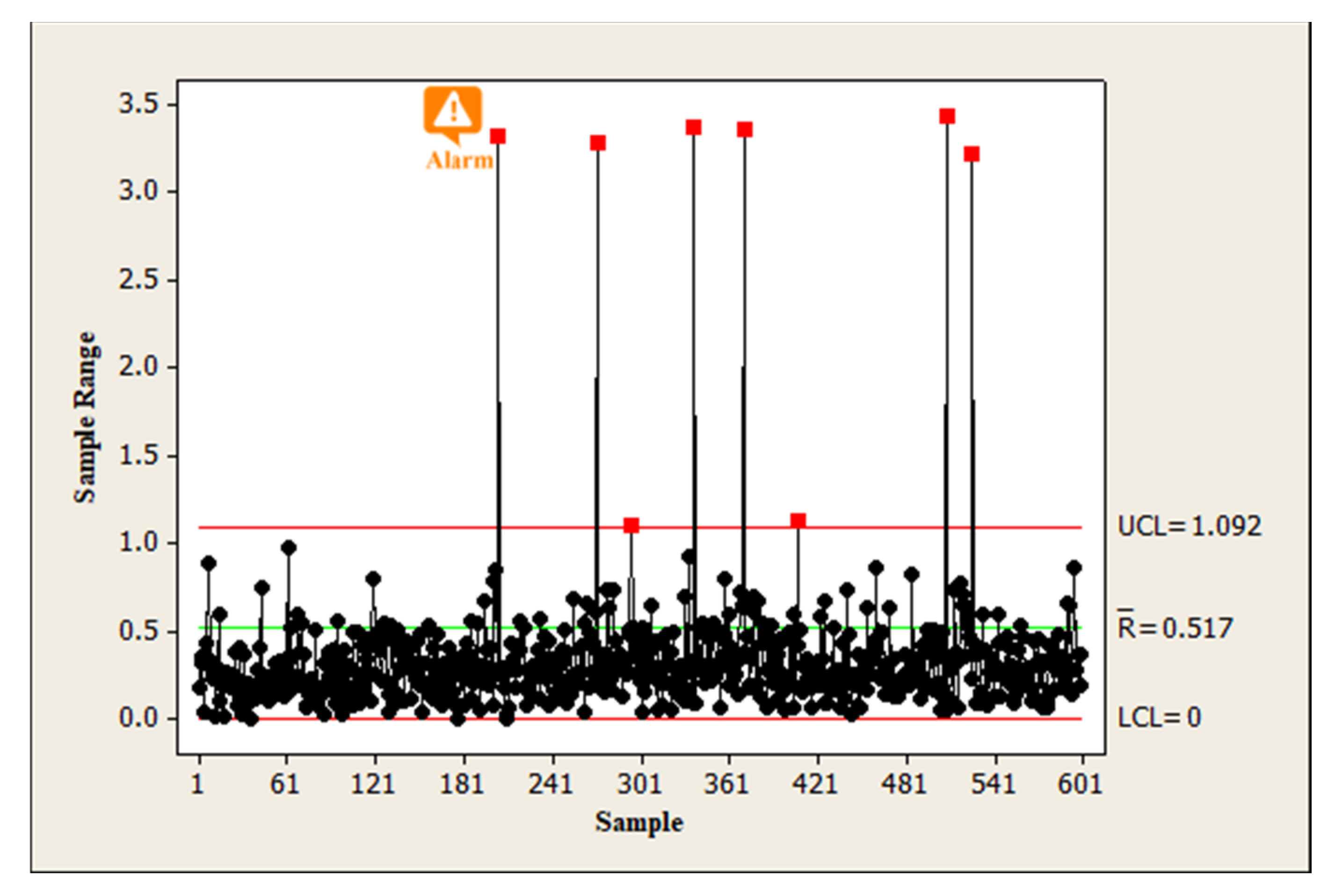
R-control chart as in Figure 14 is used to simplify the representation of the CUSUM results depicted in Figure 13 (lower chart).

As depicted in Figure 13 (upper chart), during the state change occurrence, the CUSUM of the log-likelihood ratio ($g\left(k\right)$) start increasing. Larger efficiency degradation indicates a higher slope. On the other hand, it can be seen in Figure 13 (lower chart) and Figure 14 that eight points are located in the out-of-control region (out of the upper control limit—UCL); these points represent the stopping alarms detected using the CUSUM. The first stopping alarm is triggered when the first state change is detected using the CUSUM; the other alarms indicate the continuous degradation in the gearbox efficiency as the slope increases, as shown in Figure 13 (upper chart).

The threshold $h$ was selected to avoid false alarms. However, a change detection time delay $D$ might occur accordingly, as seen in Equation (18). Thus, there is a trade-off between the false alarms and the detection time.

$$D={\mathrm{k}}_{\mathrm{a}}-k$$

(18)

Table 9. Parameters description and performance monitoring results based on CUSUM algorithm.

Parameter	Description	Value
${\mu }_0$	Normal state mean (Operating mode 1)	1.078
${\mu }_1$	Abnormal state mean (Operating modes 2 and 3)	−2.263
${\sigma }^2$	Normal state standard deviation	22.498
h	User-defined threshold (Equation (14))	3.459
$k_a$	Stopping time (first alarm) (Equation (15))	1018
${\widehat{k}}_0$	Change occurrence time (Equation (16))	969
$D$	Change detection time delay (Equation (18))	18

below summarises the performance monitoring results of the evaluated ANN power residuals for the three operating modes based on the gearbox efficiency degradation.

The monitoring method based on ANN predictions and CUSUM algorithm developed for the state change detection of gearbox efficiency offers a reliable analysis of the power generation process. This methodology also provides an early warning system for performance and condition monitoring, which helps prevent severe failure occurrences that might lead to long shutdowns of the WT. It is worth mentioning that triggering early alarms in advanced stages (${\widehat{k}}_0$) is an important indicator that can be used by the maintenance crew for better maintenance action decision-making. The process state based on the triggered alarms should be further investigated by the maintenance expert to eliminate the root causes of the detected state change. In our case, the detected state change resulted from the degraded gearbox efficiency leading to a degraded power generation process.

As indicated in the performance monitoring results, the first state change alarm ${\mathrm{k}}_{\mathrm{a}}$ and the estimated state change occurrence time (early warning) ${\widehat{k}}_0$ helps the maintenance expert to respond effectively and make decisions; accordingly, this helps in reducing the effects of unexpected shutdowns and maintenance costs as well

In summary, the monitoring results of the power prediction ANN model can be used as an efficient tool to monitor the performance of the WT by analysing the triggered alarms and the existing power residuals, which probably indicate abnormal variations of the WT performance. Moreover, the monitoring results can be used for further analysis, such as fault detection and prediction. On the other hand, the results of the gearbox efficiency prediction ANN model can be used in two ways. First, comparing the predicted gearbox efficiency in a specific time frame with a threshold provided by the manufacturer to monitor the efficiency degradation over time. Secondly, the remaining useful life of the gearbox based on its efficiency over several time cycles can be estimated based on the predicted and expected efficiencies and the efficiency threshold provided by the manufacturer. This helps in performing better maintenance plans and schedules.

4. Conclusions and Future Work

In this study, two ANN models were developed with different network architectures, designs and training algorithms. These models were able to predict the generated power of a WT based on the wind speed and gearbox efficiency, in addition to predicting the level of degradation in the gearbox efficiency based on the input wind speed and generated power.

Power residuals were calculated from the selected power prediction ANN model with the smallest average RMSE value of 0.0194. A methodology of power residuals prediction combined with a CUSUM change detection algorithm was proposed, analysed and presented to monitor the change of operating modes. This methodology is based on the power residuals resulting from the prediction ANN model and the available SCADA data of other operational modes having different gearbox efficiencies resulting in different degradation levels of power generation and different power curve profiles. The importance analysis approach was used to evaluate the importance of each input variable on the outputs for both prediction cases; wind speed is the most influential variable with 97% and 54% importance for the two models, respectively. Without real data, simulation procedures were used to generate SCADA data (power and wind speed). Combined with the developed ANN models, the recursive form of the CUSUM algorithm demonstrated an efficient way to monitor the performance of the WT and assist in detecting efficiency degradation changes. The results show that the proposed method is efficient and accurate in monitoring and detecting the state changes of operating modes. The monitoring results can be integrated and visualised using an appropriate graphical user interface (GUI) to facilitate the monitoring process of the early warnings, alarms, and the general status of the WT by the maintenance experts, which can then respond promptly to any observed change in the state of the monitored WT component without affecting the overall operations. One of the contributions of this work is modelling the SCADA data of wind speed and the gearbox efficiency to predict the generated power using an ANN-NBN model, which can train networks with full connections and arbitrary connections rather than the traditional MLP network design; this allows effective modelling of a component or even a system with complex structures of connections providing a huge amount of maintenance data. Future research could be carried out by utilising tools for developing failure detection, prediction and identification models using other appropriate types of real SCADA data towards the full implementation of the PdM strategy. Additionally, the output of the monitoring process can be used for failure classification problems.

References

1. IEA. World Energy Outlook 2019—Analysis. 2019. Available online: https://www.iea.org/reports/world-energy-outlook-2019 (accessed on 27 October 2020).
2. Benbouzid, M.; Berghout, T.; Sarma, N.; Djurović, S.; Wu, Y.; Ma, X. Intelligent condition monitoring of wind power systems: State of the art review. Energies 2021, 14, 5967. [Google Scholar] [CrossRef]
3. Abd-Elwahab, K.T.; Hassan, A.A. SCADA data as a powerful tool for early fault detection in wind turbine gearboxes. Wind Eng. 2020, 1, 1317–1326. [Google Scholar] [CrossRef]
4. Feng, J.; Shen, W.Z. Design optimization of offshore wind farms with multiple types of wind turbines. Appl. Energy 2017, 205, 1283–1297. [Google Scholar] [CrossRef]
5. Fu, J.; Chu, J.; Guo, P.; Chen, Z. Condition Monitoring of Wind Turbine Gearbox Bearing Based on Deep Learning Model. IEEE Access 2019, 7, 57078–57087. [Google Scholar] [CrossRef]
6. Tchakoua, P.; Wamkeue, R.; Ouhrouche, M.; Slaoui-Hasnaoui, F.; Tameghe, T.; Ekemb, G. Wind Turbine Condition Monitoring: State-of-the-Art Review, New Trends, and Future Challenges. Energies 2014, 7, 2595–2630. [Google Scholar] [CrossRef] [Green Version]
7. Abichou, B.; Flórez, D.; Sayed-Mouchaweh, M.; Toubakh, H.; François, B.; Girard, N. Fault Diagnosis Methods for Wind Turbines Health Monitoring: A Review. In Proceedings of the European Conference of the Prognostics and Health Management Society, Nantes, France, 8–10 July 2014; pp. 1–8. [Google Scholar] [CrossRef]
8. Stetco, A.; Dinmohammadi, F.; Zhao, X.; Robu, V.; Flynn, D.; Barnes, M.; Keane, J.; Nenadic, G. Machine learning methods for wind turbine condition monitoring: A review. Renew. Energy 2019, 133, 620–635. [Google Scholar] [CrossRef]
9. Butler, S.; O’Connor, F.; Farren, D.; Ringwood, J. A feasibility study into prognostics for the main bearing of a wind turbine. In Proceedings of the 2012 IEEE International Conference on Control Applications, Dubrovnik, Croatia, 3–5 October 2012. [Google Scholar] [CrossRef]
10. Salameh, J.P.; Cauet, S.; Etien, E.; Sakout, A.; Rambault, L. Gearbox condition monitoring in wind turbines: A review. Mech. Syst. Signal Process. 2018, 111, 251–264. [Google Scholar] [CrossRef]
11. Jin, X.; Xu, Z.; Qiao, W. Condition monitoring of wind turbine generators using SCADA data analysis. IEEE Trans. Sustain. Energy 2021, 12, 202–210. [Google Scholar] [CrossRef]
12. Schlechtingen, M.; Santos, I.; Achiche, S. Wind turbine condition monitoring based on SCADA data using normal behavior models. Part 1: System description. Appl. Soft Comput. J. 2013, 13, 259–270. [Google Scholar] [CrossRef]
13. Schlechtingen, M.; Santos, I.F. Wind turbine condition monitoring based on SCADA data using normal behavior models. Part 2: Application examples. Appl. Soft Comput. J. 2014, 14, 447–460. [Google Scholar] [CrossRef]
14. Zaher, A.; McArthur, S.; Infield, D.; Patel, Y. Online wind turbine fault detection through automated SCADA data analysis. Wind Energy 2009, 12, 574–593. [Google Scholar] [CrossRef]
15. Zhang, Z.Y.; Wang, K.S. Wind turbine fault detection based on SCADA data analysis using ANN. Adv. Manuf. 2014, 2, 70–78. [Google Scholar] [CrossRef] [Green Version]
16. Yang, W.; Court, R.; Jiang, J. Wind turbine condition monitoring by the approach of SCADA data analysis. Renew. Energy 2013, 53, 365–376. [Google Scholar] [CrossRef]
17. Shaheen, B.W.; Hanieh, A.; Németh, I. Fault detection of a wind turbine’s gearbox, based on power curve modeling and an on-line statistical change detection algorithm. Acta Polytech. Hung. 2021, 18, 175–196. [Google Scholar] [CrossRef]
18. Cabus, J.E.U.; Cui, Y.; Tjernberg, L.B. An Anomaly Detection Approach Based on Autoencoders for Condition Monitoring of Wind Turbines. In Proceedings of the 2022 17th International Conference on Probabilistic Methods Applied to Power Systems, PMAPS, Manchester, UK, 12–15 June 2022. [Google Scholar] [CrossRef]
19. Dao, P.B. Condition monitoring and fault diagnosis of wind turbines based on structural break detection in SCADA data. Renew. Energy 2022, 185, 641–654. [Google Scholar] [CrossRef]
20. Wang, K.S.; Sharma, V.; Zhang, Z.Y. SCADA data based condition monitoring of wind turbines. Adv. Manuf. 2014, 2, 61–69. [Google Scholar] [CrossRef] [Green Version]
21. Hu, A.; Xiang, L.; Zhu, L. An engineering condition indicator for condition monitoring of wind turbine bearings. Wind Energy 2020, 23, 207–219. [Google Scholar] [CrossRef]
22. Long, H.; Wang, L.; Zhang, Z.; Song, Z.; Xu, J. Data-Driven Wind Turbine Power Generation Performance Monitoring. IEEE Trans. Ind. Electron. 2015, 62, 6627–6635. [Google Scholar] [CrossRef]
23. Chen, B.; Zappalá, D.; Crabtree, C.; Tavner, P.J. Survey of Commercially Available SCADA Data Analysis Tools for Wind Turbine Health Monitoring; Technical Report; Durham University School of Engineering and Computing Sciences: Durham, UK, 2014. [Google Scholar]
24. García Márquez, F.P.; Tobias, A.M.; Pinar Pérez, J.M.; Papaelias, M. Condition monitoring of wind turbines: Techniques and methods. Renew. Energy 2012, 46, 169–178. [Google Scholar] [CrossRef]
25. Hsu, J.Y.; Wang, Y.; Lin, K.; Chen, M.; Hsu, J.H.Y. Wind turbine fault diagnosis and predictive maintenance through statistical process control and machine learning. IEEE Access 2020, 8, 23427–23439. [Google Scholar] [CrossRef]
26. Kusiak, A.; Li, W. The prediction and diagnosis of wind turbine faults. Renew. Energy 2011, 36, 16–23. [Google Scholar] [CrossRef]
27. Godwin, J.L.; Matthews, P.C. Classification and detection of wind turbine pitch faults through SCADA data analysis. Int. J. Progn. Health Manag. Spec. Issue Wind Turbine PHM 2013, 4. Available online: http://dro.dur.ac.uk (accessed on 28 March 2020). [CrossRef]
28. Tao, L.; Siqi, Q.; Zhang, Y.; Shi, H. Abnormal Detection of Wind Turbine Based on SCADA Data Mining. Math. Probl. Eng. 2019, 2019, 5976843. [Google Scholar] [CrossRef] [Green Version]
29. Yuan, T.; Sun, Z.; Ma, S. Gearbox fault prediction of wind turbines based on a stacking model and change-point detection. Energies 2019, 12, 4224. [Google Scholar] [CrossRef] [Green Version]
30. Li, G.; Wang, C.; Zhang, D.; Yang, G. An Improved Feature Selection Method Based on Random Forest Algorithm for Wind Turbine Condition Monitoring. Sensors 2021, 21, 5654. [Google Scholar] [CrossRef]
31. Corley, B.; Koukoura, S.; Carroll, J.; McDonald, A. Combination of Thermal Modelling and Machine Learning Approaches for Fault Detection in Wind Turbine Gearboxes. Energies 2021, 14, 1375. [Google Scholar] [CrossRef]
32. Amruthnath, N.; Gupta, T. A Research Study on Unsupervised Machine Learning Algorithms for Early Fault Detection in Predictive Maintenance. In Proceedings of the 2018 5th International Conference on Industrial Engineering and Applications, ICIEA, Singapore, 26–28 June 2018; pp. 355–361. [Google Scholar] [CrossRef]
33. Hameed, Z.; Hong, Y.; Cho, Y.; Ahn, S.; Song, C.K. Condition monitoring and fault detection of wind turbines and related algorithms: A review. Renew. Sustain. Energy Rev. 2009, 13, 1–39. [Google Scholar] [CrossRef]
34. Cui, Y.; Bangalore, P.; Bertling Tjernberg, L. A fault detection framework using recurrent neural networks for condition monitoring of wind turbines. Wind Energy 2021, 24, 1249–1262. [Google Scholar] [CrossRef]
35. Wang, F.; Xiao, X.; Zhao, H. Wind turbine gearbox failure prediction based on Time Series analysis and Statistical Process Control. Adv. Mater. Res. 2012, 347–353, 2236–2240. [Google Scholar] [CrossRef]
36. Wang, H.; Wang, H.; Jiang, G.; Li, J.; Wang, Y. Early fault detection of wind turbines based on operational condition clustering and optimized deep belief network modeling. Energies 2019, 12, 984. [Google Scholar] [CrossRef] [Green Version]
37. Borchersen, A.B.; Kinnaert, M. Model-based fault detection for generator cooling system in wind turbines using SCADA data. Wind Energy 2016, 19, 593–606. [Google Scholar] [CrossRef]
38. Shaheen, B.W. Model-Based Fault Detection in Wind Turbines. MSc. Thesis, Université Libre de Bruxelles and Birzeit University, Bruxelles, Belgium, Birzeit, Palestine, 2017. [Google Scholar]
39. Main Characteristics of DeWindD6. Available online: https://en.reselite.de/wind-turbine/used-for-sale/de-wind-d6-1250kw-1.25mw-1 (accessed on 27 October 2020).
40. Guo, P.; Infield, D. Wind Turbine Power Curve Modeling and Monitoring with Gaussian Process and SPRT. IEEE Trans. Sustain. Energy 2020, 11, 107–115. [Google Scholar] [CrossRef] [Green Version]
41. Paturi, U.M.R.; Cheruku, S. Application and performance of machine learning techniques in manufacturing sector from the past two decades: A review. Mater. Today Proc. 2020, 38, 2392–2401. [Google Scholar] [CrossRef]
42. Ak, R.; Li, Y.; Vitelli, V.; Zio, E. A genetic algorithm and neural network technique for predicting wind power under uncertainty. Chem. Eng. Trans. 2013, 33, 925–930. [Google Scholar] [CrossRef]
43. Javed, K.; Gouriveau, R.; Zemouri, R.; Zerhouni, N. Improving data-driven prognostics by assessing predictability of features. Progn. Health Manag. Soc. 2011, 3, 555–560. [Google Scholar]
44. Mahamad, A.K.; Saon, S.; Hiyama, T. Predicting remaining useful life of rotating machinery based artificial neural network. Comput. Math. Appl. 2010, 60, 1078–1087. [Google Scholar] [CrossRef] [Green Version]
45. Medjaher, K.; Tobon-Mejia, D.; Zerhouni, N. Remaining useful life estimation of critical components with application to bearings. IEEE Trans. Reliab. 2012, 61, 292–302. [Google Scholar] [CrossRef]
46. Ramasso, E.; Placet, V.; Gouriveau, R.; Boubakar, L.; Zerhouni, N. Health assessment of composite structures in unconstrained environments using partially supervised pattern recognition tools. In Proceedings of the Annual Conference of the Prognostics and Health Management Society 2012, PHM 2012, Minneapolis, MN, USA, 23–27 September 2012; pp. 17–27. [Google Scholar]
47. Yan, J.; Lee, J. Degradation assessment and fault modes classification using logistic regression. J. Manuf. Sci. Eng. Trans. ASME 2005, 127, 912–914. [Google Scholar] [CrossRef]
48. Carvalho, T.P.; Soares, F.A.A.M.N.; Vita, R.; Francisco, R.d.P.; Basto, J.P.; Alcala, S.G.S. A systematic literature review of machine learning methods applied to predictive maintenance. Comput. Ind. Eng. 2019, 137, 106024. [Google Scholar] [CrossRef]
49. Cotton, N.; Wilamowski, B.; Yu, H. NBN Algorithm. In Industrial Electronics Handbook, 2nd ed.; Intelligent Systems CRC Press: Boca Raton, FL, USA, 2011; pp. 1–24. [Google Scholar]
50. Yu, H.; Wilamowski, B.M. Fast and Efficient and Training of Neural Networks. In Proceedings of the 3rd International Conference on Human System Interaction, Rzeszow, Poland, 13–15 May 2010; pp. 175–181. [Google Scholar]
51. Shaheen, B.; Németh, I. Machine Learning Approach for Degradation Path Prediction Using Different Models and Architectures of Artificial Neural Networks. Period. Polytech. Mech. Eng. 2022, 66, 244–252. [Google Scholar] [CrossRef]
52. Wilamowski, B.M.; Yu, H. Improved Computation for Levenberg—Marquardt Training. IEEE Trans. Neural Netw. 2010, 21, 930–937. [Google Scholar] [CrossRef] [PubMed]
53. Wilamowski, B.M. Advanced Learning Algorithms. In Proceedings of the International Conference on Intelligent Engineering Systems, Barbados, 16–18 April 2009; pp. 9–17. [Google Scholar]
54. Wilamowski, B.M. Neural network architectures and learning algorithms. IEEE Ind. Electron. Mag. 2009, 3, 56–63. [Google Scholar] [CrossRef]
55. Wilamowski, B.M.; Cotton, N.J. Method of computing gradient vector and Jacobean matrix in arbitrarily connected neural networks. In Proceedings of the 2007 IEEE International Symposium on Industrial Electronics, Vigo, Spain, 4–7 June 2007. [Google Scholar] [CrossRef]
56. Yu, H.; Wilamowski, B.M. C++ implementation of neural networks trainer. In Proceedings of the 2009 International Conference on Intelligent Engineering Systems, INES 2009, Barbados, 16–18 April 2009; pp. 257–262. [Google Scholar] [CrossRef]
57. Blanke, M.; Kinnaert, M.; Lunze, J.; Staroswiecki, M. Diagnosis and Fault-Tolerant Control; Springer: Berlin/Heidelberg, Germany, 2003. [Google Scholar]
Figure 1. The proposed performance monitoring algorithm.
Processes 11 00269 g001
Figure 2. Ten minutes average sample simulated wind speed 2–18 m/s.
Processes 11 00269 g002
Figure 3. Simplified cause-and-effect diagram of the main problem considered in this study.
Processes 11 00269 g003
Figure 4. Gearbox efficiency degradation levels and Box plot of the simulated generated power for different operating modes.
Processes 11 00269 g004
Figure 5. Power curve profiles of a generated measurements sample. Operating modes 2 and 3.
Processes 11 00269 g005
Figure 6. ANN architectures for power predictions. (A) 2 inputs, 1 output FCN; (B) 2 inputs, 1 output MLP 2-2-1 (N is the neuron index).
Processes 11 00269 g006
Figure 7. ANN architectures for gearbox efficiency prediction. (A): 2 inputs, 1 output FCN; (B): 2 inputs, 1 output MLP 2-2-1 (N is the neuron index).
Processes 11 00269 g007
Figure 8. Importance analysis results for different input features; left figure: for power prediction, right figure: for gearbox efficiency prediction.
Processes 11 00269 g008
Figure 9. Sample of the normalised measured power and predicted power by ANN model II and their residuals.
Processes 11 00269 g009
Figure 10. Power residual distributions for all operating modes using ANN model II.
Processes 11 00269 g010
Figure 11. CUSUM change detection algorithm flow chart.
Processes 11 00269 g011
Figure 12. Change indicator of the log-likelihood ratio of the ANN power residuals.
Processes 11 00269 g012
Figure 13. Recursive CUSUM decision function: without re-initialisation (upper chart) and with re-initialisation (lower chart).
Processes 11 00269 g013
Figure 14. R-control chart of the recursive CUSUM decision function (subgroup size = 5).
Processes 11 00269 g014