Article

Multi-Task Multi-Agent Reinforcement Learning for Real-Time Scheduling of a Dual-Resource Flexible Job Shop with Robots

1
Key Laboratory of Advanced Manufacturing and Intelligent Technology, Ministry of Education, Harbin University of Science and Technology, Harbin 150080, China
2
College of Computer Science and Technology, Harbin University of Science and Technology, Harbin 150080, China
*
Author to whom correspondence should be addressed.
Processes 2023, 11(1), 267; https://doi.org/10.3390/pr11010267
Submission received: 28 December 2022 / Revised: 7 January 2023 / Accepted: 11 January 2023 / Published: 13 January 2023

Abstract

:
In this paper, a real-time scheduling problem of a dual-resource flexible job shop with robots is studied. Multiple independent robots and their supervised machine sets form their own work cells. First, a mixed integer programming model is established, which considers the scheduling problems of jobs and machines in the work cells, and of jobs between work cells, based on the process plan flexibility. Second, in order to make real-time scheduling decisions, a framework of multi-task multi-agent reinforcement learning based on centralized training and decentralized execution is proposed. Each agent interacts with the environment and completes three decision-making tasks: job sequencing, machine selection, and process planning. In the process of centralized training, the value network is used to evaluate and optimize the policy network to achieve multi-agent cooperation, and the attention mechanism is introduced into the policy network to realize information sharing among multiple tasks. In the process of decentralized execution, each agent performs multiple task decisions through local observations according to the trained policy network. Then, observation, action, and reward are designed. Rewards include global and local rewards, which are decomposed into sub-rewards corresponding to tasks. The reinforcement learning training algorithm is designed based on a double-deep Q-network. Finally, the scheduling simulation environment is derived from benchmarks, and the experimental results show the effectiveness of the proposed method.

1. Introduction

The intelligent factory focuses on integrating advanced technologies such as the Internet, big data, and artificial intelligence with enterprise resource planning, a manufacturing execution system, and production process control [1]. The intelligent factory has self-perception, analysis, reasoning, decision, and control abilities [2]. In the rapid development of large-scale personalized manufacturing, workshop management and control systems in intelligent factories can learn independently to adapt to dynamic changes in the production process [3]. Industrial robots and artificial intelligence play a key role in improving workshop intelligence and realizing the intelligent workshop. The industrial robot, which is a resource that can transfer materials flexibly and quickly, is one of the elements in the process of intelligent transformation and is also a driver of intelligent manufacturing. At the same time, deep integration of artificial intelligence with the manufacturing system, and fast, intelligent real-time analysis based on production data effectively improve the decision ability and execution efficiency of the workshop management and control system. At the core of workshop management and control, production is directly involved in information transmission and task coordination. Its real-time optimization provides greater flexibility for the operation of the intelligent workshop, and it plays a positive role in optimizing resource allocation, improving production efficiency, and reducing costs [4].
In general, the intelligent workshop is a flexible manufacturing system composed of industrial robots, machines, and other hardware, and information acquisition and control software. In the intelligent workshop, the robot is the executor of scheduling schemes, such as the loading and unloading of jobs on the machine [5]. At the same time, the robot is also an element to be considered in scheduling optimization. The machines and robots are regarded as limited resources, and the production capacity of the workshop is constrained by both of them at the same time, which is a dual-resource constraint [6]. In addition, in a flexible manufacturing system, due to the diversification of processing methods, a job may have multiple alternative process plans. Scheduling decisions should consider not only the process plan flexibility of the job, but also the machine flexibility of the operation [7]. Therefore, in the complex and dynamically changing intelligent workshop, the workshop scheduling problem, which takes robots and machines as production resources and considers high flexibility, is a more complex flexible job shop scheduling problem (FJSP).
Extensive research has been carried out on the FJSP [8,9,10], providing possibilities for diversified and differentiated personalized mass manufacturing. At present, a large number of mathematical and metaheuristic algorithms have been developed, such as the evolutionary algorithm, ant colony algorithm, and particle swarm algorithm [11]. With scheduling application in actual production, researchers have expanded the scheduling problem according to different scenarios. Among them, the integration of process planning and scheduling issues has received a great deal of attention [12,13]. The FJSP with flexible process planning is a more complex decision problem. Özgüven et al. [14] developed a mixed integer programming model for FJSP with flexible process planning, which created an effective mathematical model. Phanden et al. [15] summarized three solutions for process planning and scheduling integration: non-chain, closed-loop, and distributed. In the above research, the scheduling problems mostly focused on the machines. However, the operation process requires not only machines, but also other types of resources, such as robots, workers, logistics equipment, and fixtures. Brucker et al. [16] studied the cyclic job–shop problem with transportation for optimization problems in fully automated manufacturing systems or assembly lines. They characterized feasible solutions based on the route of the robot and their properties. To optimally minimize the cycle time, a tree search method was developed to construct feasible solutions. Fatemi-Anaraki et al. [17] investigated a dynamic scheduling problem within a job shop robotic cell, wherein multiple robotic arms are responsible for material handling in a U-shaped arrangement. They also designed a mixed integer linear programming model and solution method for this problem. Ham [18] studied the simultaneous scheduling of production and material transfer in a FJSP environment. Two different constraint programming formulations are proposed for the FJSP with a robotic mobile fulfillment system. Analysis results show significant outperformance of all other benchmark approaches in the literature. The above literature shows that in intelligent workshops, machines and robots have gradually become the main production resources. This is more complex than the scheduling problem of a single resource [19].
The existing literature has studied different FJSPs with dual-resource constraints. Wu et al. [20] considered fixtures and machines as two kinds of resources and studied the FJSP with dual-resource constraints considering fixture loading and unloading. The research results showed that the scheduling scheme with multiple resources had a greater guiding role in production than the scheduling scheme with a single resource. He et al. [21] constructed a dual-resource constrained FJSP model with machine and worker. An improved African vulture optimization algorithm is developed such that the makespan and total delay are minimized. Jiang et al. [22] presented a discrete animal migration optimization to solve the dual-resource constrained energy-saving FJSP to minimize the total energy consumption in the workshop. Results demonstrate that the proposed algorithm has advantages against other compared algorithms in terms of the solving accuracy for solving the studied scheduling problem. Hongyu et al. [23] focused on three kinds of indicators of sustainable development—that is, economy, environment, and society—and schedule two types of resource—that is, machines and workers—simultaneously in the classical FJSP. An improved survival duration-guided NSGA-III algorithm is proposed to solve the problem. These studies assume that each worker can only operate one machine; that is, the dual-resource constraint problem with a single task and simultaneous supervision. However, in an intelligent workshop, robots generally serve multiple machines at the same time, which is called the dual-resource constraint problem with multiple tasks and simultaneous supervision (MTSSDRC). This can effectively improve productivity [24]. In this kind of scheduling problem, completing a job operation involves at least three activities: loading, processing, and unloading. The loading and unloading are carried out by the robot before and after processing, and the processing is completed by the machine.
At present, the literature on the MTSSDRC scheduling problem is limited. Costa et al. [25] and Akbar et al. [26,27] proposed a dual-resource constrained parallel machine scheduling problem, in which workers execute activities between machines. It makes up for the multi-worker supervision problem, which is usually ignored in traditional dual-resource scheduling, and establishes a mixed integer linear programming mathematical model. Later, Akbar et al. [28] improved several metaheuristic algorithms for the proposed model, making it suitable for solving MTSSDRC scheduling problems. The above literature laid a foundation for the MTSSDRC, and the algorithms are all suitable for solving the parallel machine scheduling problem. Research on the FJSP considering the MTSSDRC is scarce, which made it difficult to solve the scheduling problem proposed in this paper.
In the mass customization environment, the changing order and machine state are highly flexible, and the scheduling decision system needs to conduct adaptive self-optimization for such a dynamically changing workshop environment [29]. Therefore, the real-time generation of scheduling schemes becomes very important. Scheduling solutions based on mathematical modeling, the heuristic algorithm, the metaheuristic algorithm, and other algorithms [30,31,32] require iterative calculation and show poor real-time performance. Priority-based scheduling rules can effectively improve real-time decision-making. Choosing different priority rules according to dynamic changes is usually better than using a single priority rule. Therefore, the current related studies are focused on scheduling policies involving the dynamic selection of priority rules. This type of scheme completes the development of the scheduling policy through offline training, and then carries out high-quality and real-time scheduling online. Commonly used methods include genetic programming, machine learning (ML), and reinforcement learning (RL). The genetic programming method is carried out through iteration and population evolution. The disadvantage of this method is that it takes time to check the performance of candidate rule sets, which reduces the real-time scheduling. ML is used as a data mining tool to mine the historical data of the workshop. Based on the supervised learning method of classified tasks, appropriate scheduling rules are selected according to the real-time state of the workshop [33,34,35]. Different from ML, RL can establish direct mapping from environmental states to actions. Furthermore, deep reinforcement learning (DRL) using neural networks as value or policy functions can also handle complex tasks. These characteristics make DRL a more effective method for scheduling research in complex flexible manufacturing systems.
At present, DRL is widely used in workshop scheduling, such as for single machines, parallel machines, flow shop, and job shop. Generally, the scheduling rules used to solve the FJSP can be divided into two types: job selection rules and machine selection rules. For these two types of rules, scholars have defined FJSP as a Markov decision process (MDP) and used DRL for scheduling research. Luo [36] studied the dynamic FJSP under the condition of new job insertion with the objective of minimizing total tardiness. A real-time scheduling method based on the deep Q-network (DQN) was designed and used to select appropriate actions at scheduling decision points and complete the selection of jobs and machines. The research results show that the proposed method had better advantages and versatility compared to various combination rules, classical scheduling rules, and standard Q-learning. Han et al. [37] proposed an end-to-end DRL framework to solve the FJSP. In this framework, according to selected scheduling characteristics, pointer networks are used to encode scheduling operations, and a recursive neural network is used to model the decoding network. The experimental results showed that this method had better performance than classical heuristic rules.
The studies above all adopted the centralized model of a single agent and assumed that it was globally observable. This method lacks flexibility and autonomy. In order to overcome this shortcoming, Luo et al. [38] proposed a real-time scheduling method based on hierarchical multi-agent DRL. This method includes three agents: scheduling objective, job selection, and machine selection agents. This method effectively solves the dynamic multi-objective FJSP with new job insertion and machine failure. Liu et al. [39] proposed a layered and distributed framework to solve the dynamic flexible job shop scheduling problem. Based on the double-deep Q-network (DDQN), the machine selection agent and job sequencing agent are trained to make real-time scheduling decisions for the FJSP with the job deadline. Johnson et al. [40] proposed a DDQN-based multi-agent reinforcement learning method to solve the FJSP problem of robot assembly cells. Each agent in the assembly unit is trained in a centralized way and executes scheduling decisions independently according to local observations. The experimental results showed that this method had good performance in optimizing the maximum completion time.
However, in the above research, each agent only performed the decision of one task, which can only be adapted to small-scale scheduling problems. In a complex workshop environment, agents often need to be able to make decisions on multiple tasks to adapt to problems on a larger scale. Therefore, agents are required to have the ability to complete multiple task decisions. Lei et al. [41] noted that in the FJSP environment, an agent needs to control multiple actions at the same time, and they proposed a multi-pointer graph network architecture and multi-optimal policy optimization training algorithm to learn action policies of machine and job selection, in order to achieve the scheduling of allocating jobs to machines. The results showed that the agent could learn high-quality scheduling strategies, outperform heuristic scheduling rules in terms of the quality of solutions, outperform metaheuristic algorithms in terms of running time, and have good generalization performance on large-scale instances. Some scholars put forward the paradigm of multi-task learning based on shared representation. Jaing et al. [42] proposed a multi-task DRL method to solve the complex 3D boxing problem. The agent task includes three subtasks: sequence, direction, and position. This method can solve more large-scale instances and was shown to have good performance. Omidshafiei et al. [43] studied the locally observable multi-task multi-agent reinforcement learning problem, introduced a distributed single task learning method, which was robust to the cooperation between agents, and proposed a method to refine the single task policy into a unified policy, which performed well in multiple related tasks.
In this paper, for the dual-resource FJSP with robots, multiple agents are required to complete the decision to improve the scheduling performance, and each agent needs to have decision-making capability for multiple tasks. This poses a challenge to the existing multi-task and multi-agent RL method, because it is necessary to design an applicable framework according to the particularity of the problem. This framework not only requires coordination between agents to obtain good performance, but also ensures the universality of all policies to make more reasonable scheduling decisions using local observations.
To sum up, in order to solve the production scheduling problem of a typical com-plex flexible manufacturing workshop, the FJSP studied in this paper considers the dual-resource constraints of robots and machines (with each robot supervising multiple machines) and flexible process planning, which is the FJSP with dual resources and process plan flexibility (FJSP-DP). A DRL method is designed to solve the real-time scheduling problem. First, the FJSP-DP problem is described, and its mixed integer programming model is established to analyze and construct the scheduling environment. Second, combining the ideas of centralized training and decentralized execution, a real-time scheduling framework for multi-task multi-agent reinforcement learning (MTMARL) based on the DDQN algorithm is designed. The robot of each work cell acts as an agent to complete the scheduling decision tasks of the corresponding cell, including job sequencing, machine selection, and process planning. The centralized training method is adopted, and the value network of each agent evaluates and optimizes the policy network of its task execution action selection by sharing local observations. The policy network is composed of multiple neural networks for training and learning multiple task decisions. Then, the state, action, reward, and learning policies required by reinforcement learning training are designed to improve the learning efficiency and performance of the agent. Considering full cooperation between agents, the rewards include global and local rewards. Based on the scheduling decision tasks that each agent must complete, local rewards are decomposed into multiple sub-rewards for training the network parameters related to each task. Then, according to the designed reinforcement learning environment and the scheduling problem, the proposed framework training algorithm is developed. Finally, the scheduling simulation environment is built, and the algorithm training and performance analysis are carried out using the designed simulation examples to verify the effectiveness of the proposed method.
This paper makes the following contributions through developing and evaluating the proposed method:
(1)
We establish the mixed integer programming model of FJSP-DP. In the model, each operation is scheduled by considering the flexibility of the process planning, the flexibility of the machine, which work cell to choose, and the loading and unloading activities.
(2)
We develop the MTMARL approach for the real-time scheduling system of FJSP-DP. The approach has the functions of centralized training and decentralized execution of scheduling decisions. Each agent independently makes decision and communicates with other agents in real-time.
(3)
We evaluate the feasibility and effectiveness of the proposed approach by developing a simulation environment of FJSP-DP and the MTMARL algorithm based on numerical experiments.
The rest of this paper is organized as follows. Section 2 describes the FJSP-DP and establishes its mixed integer programming mathematical model. In Section 3, a real-time scheduling method framework based on MTMARL is proposed. Section 4 describes the design of the state, action, reward, policy, and training method. In Section 5, numerical experiments and results analysis are presented. Finally, Section 6 summarizes the contributions of this paper and discusses future research directions.

2. Problem Description

The FJSP-DP is restricted by two kinds of resources: machines and robots. Where, the type of robot we assume is a robotic arm with a single gripper. Each of them has the same capacity regarding material handling (i.e., loading and unloading). The composition of the workshop is shown in Figure 1, with m machines and w robots (w < m). Robot k supervises the loading and unloading activities of each machine, and the machine set it supervises is { M k l } l = 1 N k   ( M k l     M ) . Robot k and the machines it supervises form a work cell (shown in Figure 1a). The buffer in the work cell is used to store jobs awaiting processing and completed jobs. There are n jobs, and the job set is J = { J i } i = 1 n . Job i has a process plan set (as shown in Figure 1b), which is denoted as P i = { O i p i } p i = 1 τ I , and j ( j O i p i ) represents the j -th operation in the p i -th process plan of job i. Each operation performs three sequential activities on the same machine: loading, processing, and unloading. After the robot completes the activity of one operation, it can perform the activity of other operations. Job i enter the corresponding work cell of each operation in turn according to its process plan until all operational activities are completed.
The relative assumptions are as follows:
(1)
Each machine or robot can only process at most one job at a time.
(2)
Each job can be processed by no more than one machine at one time.
(3)
The transport time of the job between work cells is not considered.
(4)
The buffer has unlimited capacity.
(5)
Setup time is ignored.
(6)
Rework and job loss are not considered.
(7)
Preemption is prohibited, and the machine does not interrupt.

2.1. Notation

According to the problem description, the mathematical symbols are as follows:
Parameters:
k   Index of robots (or work cells); k     W
h   Index of machines; h     M
i    Index of jobs; I     J
j    Index of operations; j   O i p i
p i     Process plan for job i; p i P i
a   ( b ,   c )  Loading or unloading activity; a   ( b ,   c )     A
M    Set of machines: M = { 1 ,   2 ,   ,   m }
M j  Set of machines available for processing operation j
W    Set of robots: W = { 1 ,   2 ,   ,   w }
J   Set of jobs: J = { 1 ,   2 ,   ,   n }
O i p i    Set of operations belonging to the p i -th process plan of job i
P i    Set of process plans belonging to job i
A     Set of activities; A = { 1 ,   2 } (1 loading, 2 unloading)
Input variables:
m     Number of machines
w  Number of robots
n   Number of jobs
D i    Deadline for job i
T i p i j h  Processing time of operation j, which belongs to the p i -th process plan of job i on machine h
T j a    Execution time of activity a of operation j
L    A large number
Decision variables:
X khjah j b  Equals 1 if robot k completes activity a of operation j on machine h, before performing activity b of operation j′ on machine h′, and 0 otherwise
Y ip i jh   Equals 1 if operation j, which belongs to the p i -th process plan of job i, is processed by machine h, and 0 otherwise
Z ip i   Equals 1 if job i select the p i -th process plan, and 0 otherwise
U jj    Equals 1 if loading of operation j performed before unloading of operation j′ on the same machine, and 0 otherwise
S ja     Starting time of active a, which belongs to operation j
C ja     Completion time of active a, which belongs to operation j
C ip i jh Completion time of operation j, which belongs to the p i -th process plan of job i on machine h
C i    Completion time of job i
C max  Makespan

2.2. Formulation

The optimization objectives of FJSP-DP mainly consider delivery time and resource load. The scheduling of delivery time is conducted to obtain a scheme with a minimum tardiness penalty, whose objective is given by Formula (1).
Minimize   i = 1 n max ( C i D i , 0 )
The resource load considers machine and robot resources. For the machine, the optimization objective is expressed as minimizing the maximum machine utilization. Its objective is given by Formula (2).
Minimize   max ( i   J p i P i j O ip i Y ip i jh T ip i jh C max )
For robots, the load of each robot is measured by calculating its total working time (total loading and unloading time).
Suppose T W k is the total working time of robot k and T W ¯ is the average total working time of all robots. Formula (3) is used to calculate the load deviation of all robots. The objective is to minimize the load deviation.
Minimize   k = 1 w ( T W k T W ¯ ) 2
s.t.,
p i P i Z ip i = 1   ( i     J )
h M j Y ip i jh = 1   ( i   J ,   p i P i ,   j O ip i )
k W h M j j O ip i a A h M j X khjah j b = 1   ( b A ,   j O i p i )
k W h M j h M j j O i p i b A X khjah j b 1   ( a   A ,   j O ip i )
k W h M j j O ip i a A X khjah j b k W h M j j O i p i c A X k h j ch j b = 0   ( h M ,   j O i p i )  
h M j j O ip i a A X khjah j b h M j j O i p i c   A X h j bh j c ( k   W ,   h   M ,   j O i p i , b   A )
{ C j 1 C j 2 k W h M j O ip i a A T j 1 X khjah j 1 L ( 2 k W h M j O ip i a A ( X khjah j 1 + X khjah j 1 ) + U j j ) C j 1 C j 2 k W h M j O ip i a A T j 1 X khjah j 1 L ( 2 k W h M j O ip i a A ( X khjah j 1 + X khjah j 1 ) + 1 U j j ) ( h M ;   j O i p i ;   j O i p i )
C ja S ja T ja   ( a   A ,   j O ip i )
S j b C ja L ( 1 k   W h M j h M j X khjah j b )   ( a ,   b   A ;   j O ip i ;   j O i p i )
C j 2 C ip i jh T j 2   ( i J ,   p i P i ,   j O ip i ,   h M j )
C ip i jh C j 1 = T ip i jh   ( i J ,   p i P i ,   j O ip i ,   h M j )
S j 1 C ( j 1 ) 2   ( j O ip i )
C 02 = 0
C i   C j 2   ( i J ;   j O ip i )
C max   C i   ( i J )
T W k = h M j j O ip i a A h M j j O i p i b A X khjah j b T j b   ( k W )
{ X khjah j b { 0 , 1 }   ( k W ;   h , h M ;   j O ip i ;   j O i p i ; a , b A ) Y ip i jh { 0 , 1 }   ( i J ;   p i P i ;   j O ip i ;   h M ) Z ip i   { 0 , 1 }   ( i J ;   p i P i ) U jj { 0 , 1 }   ( j O ip i ;   j O i p i )
Constraint (4) indicates that only one process plan can be selected for each part.
Constraint (5) imposes that each operation can only be scheduled once.
Constraint (6) specifies that any activity of any operation is only assigned to one robot and one machine, and the activity of operation j is performed after the activity of operation j is completed.
Constraint (7) imposes that the robot can only perform one activity at a time.
Constraint (8) indicates that loading and unloading activities of one operation are completed on the same machine.
Constraint (9) ensures the sequence feasibility of activities: if activity b of operation j is prior to activity c of operation j , there must be activity a of its previous operation j .
Constraint (10) ensures the sequence feasibility on each machine: if loading of operation j and unloading of operation j are processed on the same machine, unloading of operation j must be completed before loading of operation j starts, and vice versa.
Constraint (11) indicates that the activity completion time of operation j .
Constraint (12) imposes that a robot executes two adjacent activities, starting time of the activity is greater than completion time of the previous activity.
Constraint (13) indicates that after completing an operation, unloading activity can be performed.
Constraint (14) specifies that each machine starts processing operation immediately after completing loading activity.
Constraint (15) ensures that loading activity of the current operation of the same job is carried out after unloading activity of the previous operation is completed.
Constraint (16) defines the virtual operation 0 of each job, whose unloading completion time is 0, and ensures that start processing time of each job is greater than 0.
Constraint (17) defines that completion time of the job is after unloading of its last operation.
Constraint (18) defines the makespan.
Constraint (19) is used to calculate the total working time of each robot.
Constraint (20) specifies that the decision variables, including X khjah j b , Y ip i jh , Z ip I , and U jj are binary.

3. Methodology and Framework

3.1. Real-Time Scheduling Decision Tasks

3.1.1. Breakdown of Tasks

Real-time scheduling needs to consider the decisions of scheduling tasks, the scheduling rule corresponding to each decision, and the definitions of scheduling decision points. The scheduling task of FJSP-DP can be divided into two tasks:
(1)
Scheduling of the work cell: Complete the scheduling decision of allocating work pieces to the machine in the cell, which includes job sequencing and machine selection. According to the decision of job sequencing, a job will be selected in the temporary storage area queue, which determines the processing order of the job in the work cell. The machine selection decision is used to determine which machine will process the selected job. According to the priority rule of machine selection, a suitable machine is determined in the machining cell.
(2)
Scheduling between work cells: The work cells corresponding to the next operation of the completed job will be determined in the current work cell, which is determined by the priority rules of process planning. Different from the traditional process planning, which determines in advance, the next operation should be selected from the flexible process planning set according to the real-time production status under the demand of real-time scheduling.
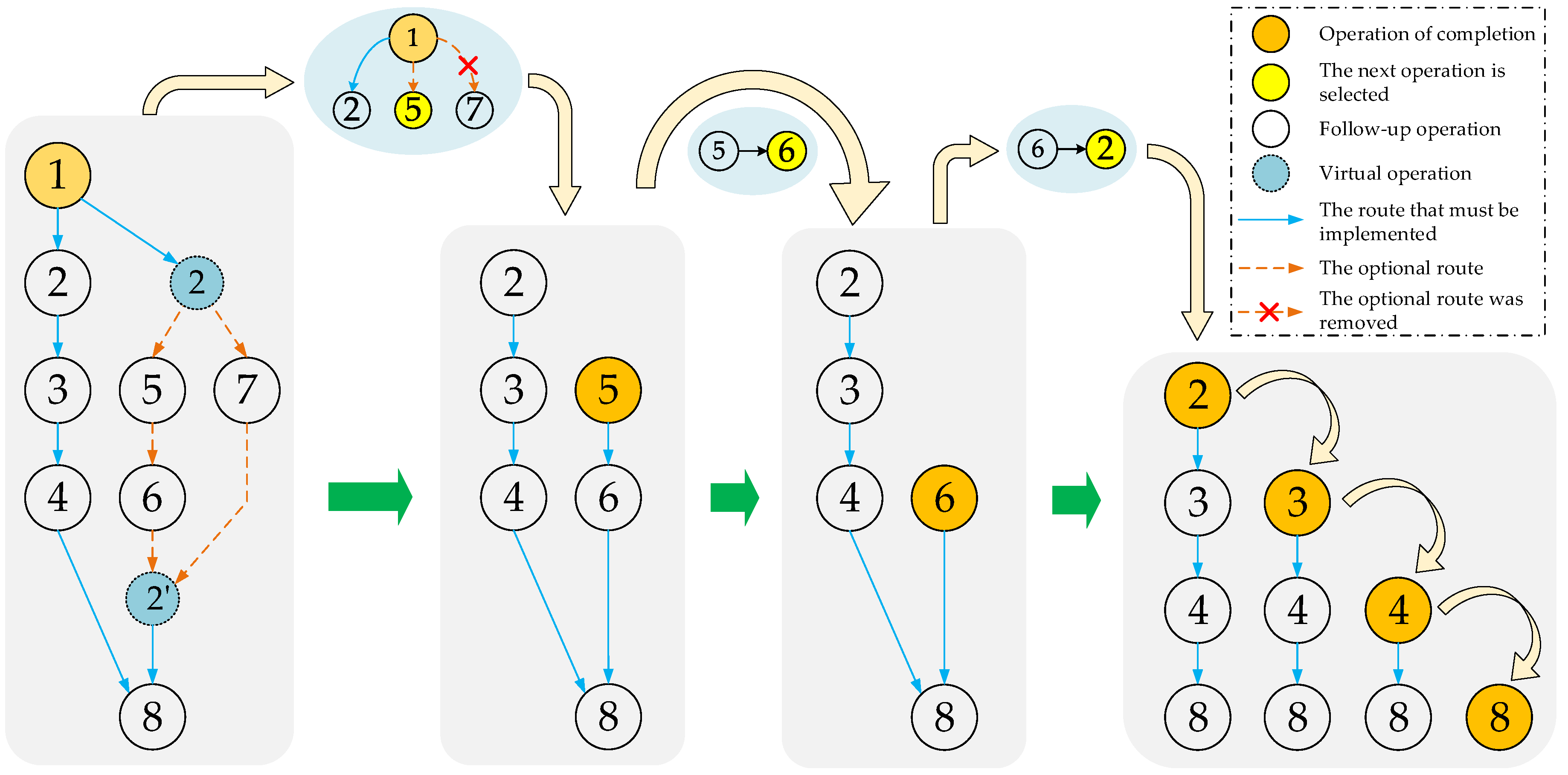
Therefore, this paper adopts the process planning method based on the operation tree [44] to build a directed graph model of dynamic process planning. Figure 1b was transformed into the directed graph model of the operation tree shown in Figure 2. Here, the operation tree is defined as follows:
(a)
There are three operation types in the operation tree: leaf operation, node operation, and root operation. Root node operation is the last operation of the job. When the root node operation is completed, the job processing is completed.
(b)
The current executable operations in the operation tree can only be leaf operations (node and root operations can only be executed if they become leaf operations). After the leaf operation is completed, it will fall off and update the operation tree.
(c)
When all leaf operations corresponding to node operations are completed and fall off from the number of operations, the node operation is converted to leaf operation and can be executed.
(d)
Redundant routes in the flexible process planning are represented by dotted lines in the operation tree. When the process planning is selected, only one redundant path can be selected for execution. The solid line in the process tree is the route that must be executed.
(e)
In order to consider the constraints between process path branches, virtual operation pairs are introduced (2, 2’), as shown in Figure 2. Operation pairs contain multiple redundant paths that can be selected.
Virtual operation 2 indicates that the operation before operation 2 must be completed before operation 5 or 7 can be processed. Virtual operation 2 indicates the end of redundant routing, and the next path can be executed.
In real-time scheduling, it is necessary to obtain the information of the next executable operation according to the operation tree. The precondition for obtaining this information is to judge the node type of the operation. Therefore, in the directed graph model of dynamic process planning, the node type is determined by the degree of output and input of nodes. If the degree of penetration is 0, it indicates a leaf node; if the degree of output or input is greater than 1, it indicates node operation; and if the output is 0, it indicates root node operation. In the directed graph, the constraint relationship between process nodes is represented by an adjacency matrix. Therefore, in real-time scheduling, the dynamic changes of the operation tree can be effectively expressed by the degree of nodes and the adjacency matrix.
In real-time scheduling, it is necessary to obtain the information of the next executable operation according to the operation tree. The precondition for obtaining the information is to judge the node type of the operation. Therefore, in the directed graph model of the dynamic process planning, the node type is determined by the degree of output and degree of input of nodes. If the degree of penetration is 0, it indicates the leaf node; If the degree of output or input is greater than 1, it indicates a node operation; If the output is 0, it indicates the root node operation. In the directed graph, the constraint relationship between process nodes is represented by the adjacency matrix. Therefore, in the real-time scheduling, the dynamic changes of the operation tree can be effectively expressed by the degree of nodes and the adjacency matrix.
This paper considers both process planning flexibility and machine operation flexibility, which ultimately determines the next operation and the corresponding work cell. Therefore, in the dynamic flexible planning process, the next operation and the required processing unit are determined as follows:
Step 1: Calculate the output of the current operation node. If the output is equal to 0, jump to step 5; if it is equal to 1, jump to step 3; and if it is greater than 1, go to step 2.
Step 2: Select the next operation to be executed from the next operation set according to the process data information and the priority rule of process planning.
Step 3: Retrieve the set of machines required for the selected next operation and divide the set of selectable processing units for that operation.
Step 4: According to the real-time status information of the processing unit, select a processing unit through the priority rule, then transfer the job to the processing unit.
Step 5: After the job is processed in the work cell, calculate the node output. If it is 0, it means the job is processed and the next work cell does not need to be selected; otherwise, go back to step 1.

3.1.2. Decision Point and Decision Flow

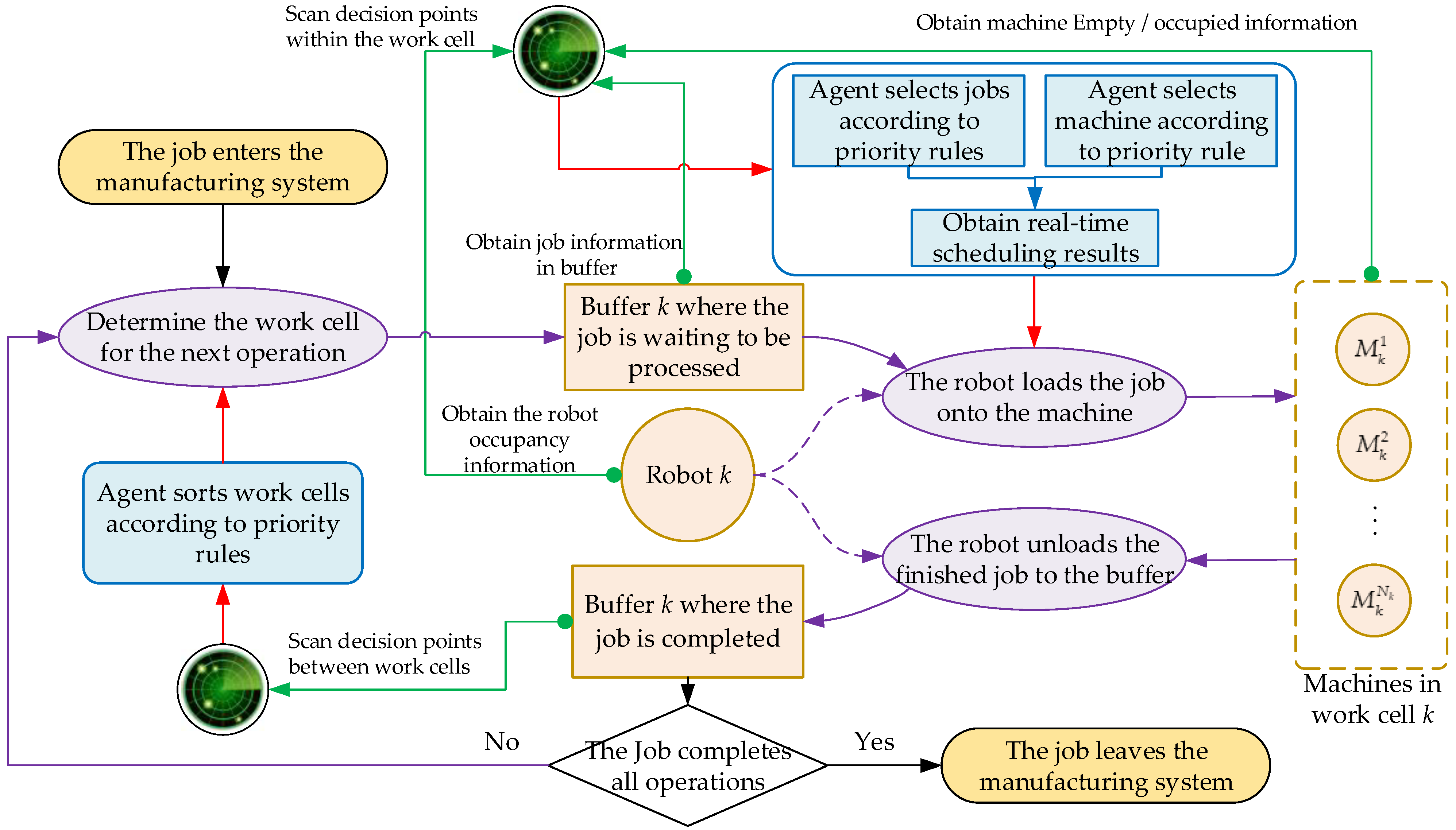
There are two decision points corresponding to the scheduling task of FJSP-DP. Due to the constraints of dual resources, scheduling in cells should take into account the occupations of robots and machines. Therefore, the designed scheduling decision point in the cell meets the following conditions: there are idle machines in a work cell, there are jobs waiting to be processed in the buffer zone, and the robot is not occupied. Scheduling between cells mainly considers the next operation of the job and its corresponding work cells. The condition of its scheduling decision point is that there are finished jobs in the staging area and the jobs have remaining operations. When the job is in the 0-th operation, a priority rule is randomly selected to complete the determination of the unit for the first operation and directly enter the unit. When the jobs in the staging area have completed all operations, they are delivered directly. No decision needs to be made for the entry and exit of the above artifacts. The priority is higher for robot unloading than loading. When multiple unload requests occur at the same time, unload in the order of first request and first unload. The execution process of the FJSP-DP scheduling decision is shown in Figure 3.

3.2. Scheduling Decision via DDQN

DQN is an effective method to solve discrete system decision problems. It combines reinforcement Q learning with the nonlinear value function, trains the neural network through reinforcement learning, and uses the neural network to approximate the Q value function, which is the policy of action selection [45,46]. DQN includes an online network (Q-Net) and a target network ( Q ^ -Net), and the output of these two networks is the Q value of the action. The experience tuple ( s t , a t , r t , s t + 1 ) generated at each time step are stored in the replay memory during the training process of the agent’s interaction with the environment. Tuple data are randomly sampled through small batch updating, and the gradient descent policy is used to modify online network parameter θ t to maximize the Q value function. The parameter update formula of online network is
θ t + 1 = θ t + η ( y t Q ( s t ,   a t ;   θ t ) ) θ Q ( s t ,   a t ;   θ t )
where η is the learning rate used by the gradient descent algorithm, θ is the gradient descent policy, and y t is the estimated target value. The iteration formula for each time step is
y t DQN = r t + 1 + γ Q ( s t + 1 ,   argmax a ( s t + 1 ,   a ;   θ ^ t ) ;   θ ^ t )
where γ is the discount factor in the Q-learning algorithm and θ ^ t is the parameter of the target network. Obviously, when DQN estimates the target value, it always selects the maximum output value of target network Q ( s t + 1 ,   a ) , which will lead to overestimation problems, could greatly reduce the learning quality of the agent, and is not conducive to the stability of learning. In order to reduce overestimation of Q value, Hassell et al. proposed DDQN based on DQN [47]. Unlike DQN, DDQN inputs the status s t + 1 to both the online and target network. First, DDQN finds the action with the maximum output value from the online network, and then the output value of the target network corresponding to the action. The Q value of the online network provides the behavior policy to select actions, and the target network output is used to evaluate the Q value of the action. Therefore, the formula for calculating the target value of DDQN estimation is
y t DDQN = r t + 1 + γ Q ( s t + 1 ,   argmax a ( s t + 1 ,   a ;   θ t ) ;   θ ^ t )
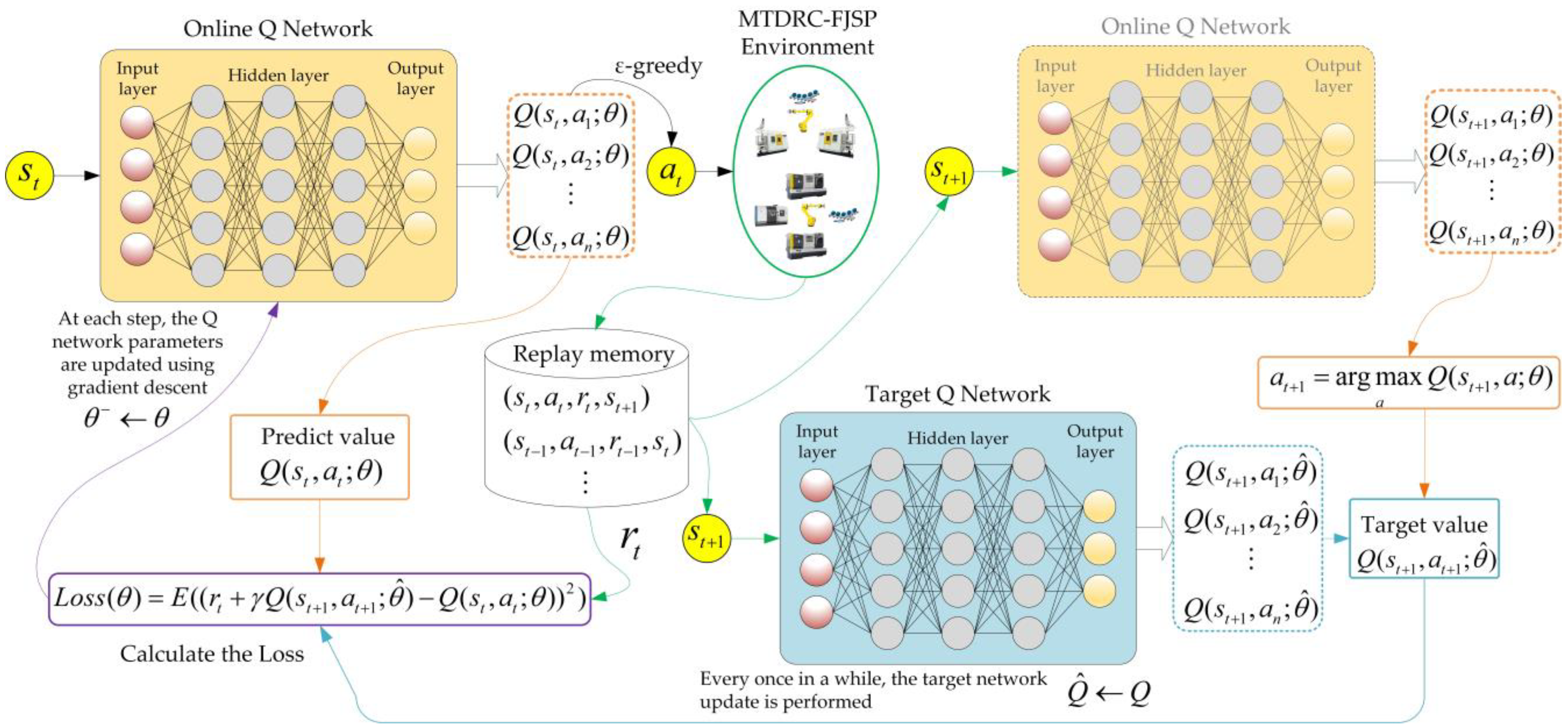
The process of agent learning and training in the scheduling environment using deep reinforcement learning based on DDQN is shown in Figure 4. The agent obtains real-time production data of the flexible job shop environment and processes the data to form a state s t . The online network obtains the Q ( s t ,   a ;   θ ) of each action according to s t , and uses the ε-greedy policy to select action a t . Action a t is converted into the corresponding scheduling rules, and then job sequencing is executed, with machine selection or process planning to make the environmental transition to the next state s t + 1 , to obtain reward r t related to the scheduling objective.
At the same time, the learning experience ( s t , a t , r t , s t + 1 ) is stored in the memory buffer. With the real-time interaction between the agent and the scheduling environment, the memory buffer is constantly updated. At each time step, a batch of scheduling decision experience data is obtained from the memory buffer, and each s t + 1 is input into the online and target networks.
The online network outputs the a t + 1 corresponding to the maximum Q value, and the target network obtains the value Q ( s t + 1 ,   a t + 1 ;   θ ) corresponding to a t + 1 , which is combined with reward r t as the target estimate y t .
Using Q ( s t ,   a ;   θ ) as the prediction value, DDQN calculates the loss function Loss(θ), and then updates the online network parameter θ according to the gradient descent policy. Therefore, once the agent interacts with the scheduling environment, the online network parameter θ will be updated once. During the continuous interaction between the agent and the scheduling environment, the target network parameter   θ ^ is occasionally updated with online network parameter θ. This interactive iteratively updating learning process makes the scheduling decision performance continuously improve.

3.3. Framework of Centralized Training and Decentralized Execution

As described in the previous section, when DDQN is used to solve the scheduling problem, it is a scenario where the agent interacts with the environment and completes the scheduling decision. In the MTMARL, the multi-agent is the subject of scheduling decisions—it can be a software system. Manufacturing resources (including robots) or computers can be the carrier of the agent. The control system of the robot can be installed with a multi-agent decision module so that the robot has scheduling decision ability. In this FJSP-DP, each robot acts as an agent and executes the agent’s decision results. Multiple agents complete their decision-making tasks by sharing local observations. The decision objectives of each agent are consistent in order to optimize the scheduling objectives and obtain the same return. Therefore, multiple agents have a full cooperative relationship. Based on the analysis of scheduling tasks, each agent should have decision ability for job sequencing, machine selection, and process planning at the same time.
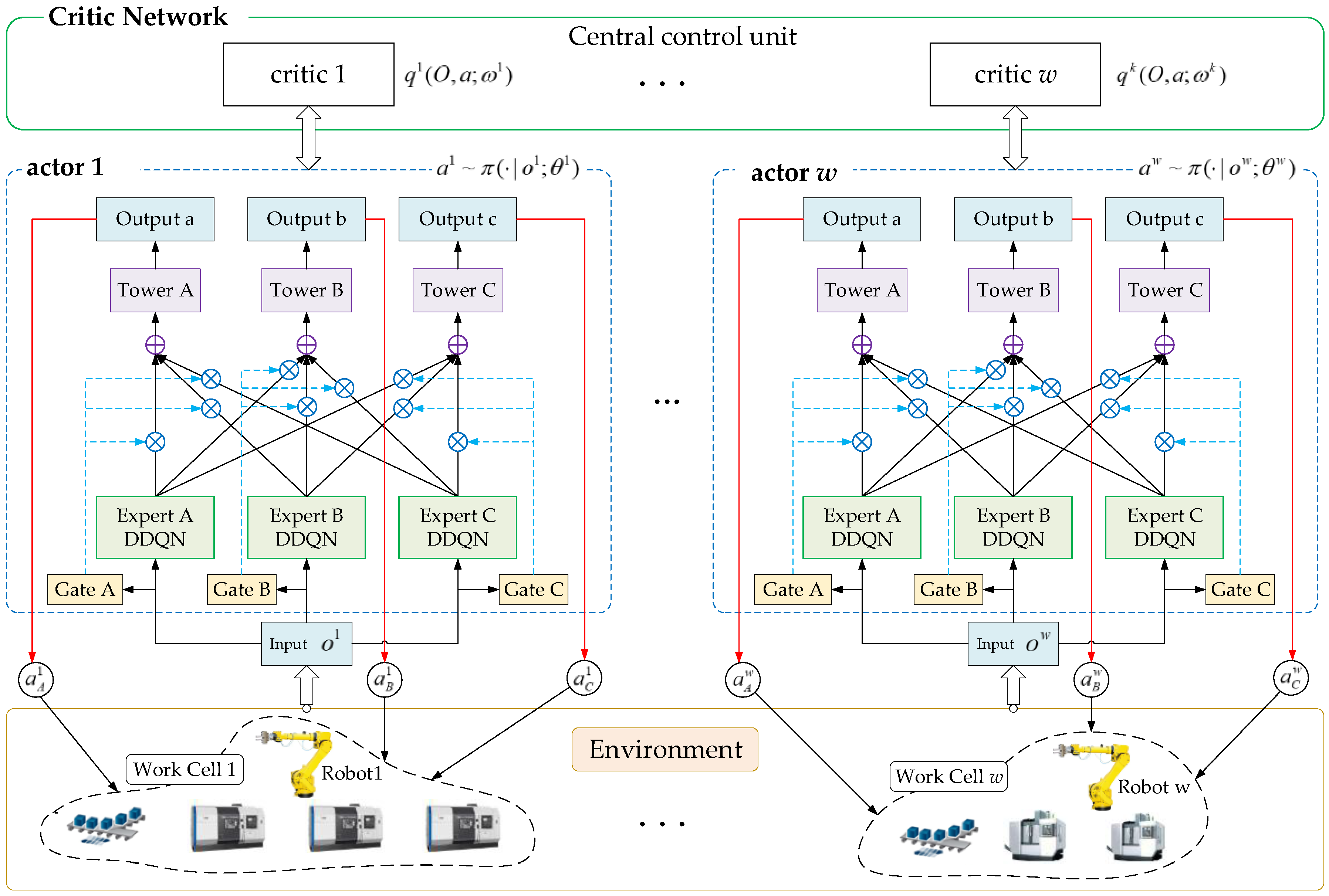
Considering the complete cooperation among multiple agents, a centralized training and decentralized execution reinforcement learning framework is adopted to solve the FJSP-DP in this paper. The framework is based on the DDQN, as shown in Figure 5. Each agent interacts with the environment by executing actions and receives feedback from the environment in the form of states and rewards. In the centralized training phase, the value of network critical k in the central controller is used to evaluate the decision actions made by agent k, which is used to train and optimize policy network actor k. In the decentralized execution phase, agent k acquires local observations o k , inputs them into its policy network actor k, and makes scheduling decisions. This decision process does not require communication between agents. This kind of decentralized decision is fast and can achieve real-time results.
There are w value networks in the central controller to evaluate the learning policies of each agent. The value network is a group of neural networks with the same structure, and the parameter w k of each neural network k may be different. These neural networks are used to fit the Q function (i.e., q k ( O ,   a ;   w k ) ) in reinforcement learning, where O = { o 1 , o 2 ,   ,   o w } is a global observation consisting of each local observation. In the process of centralized training, each agent conducts the training of the policy network ( a k ~ π   ( ·   |   o k ;   θ k ) ) by sharing their own observations. Agent k interacts with the environment, and critical k scores according to the actions given by actor k. This centralized training process realizes cooperation among multiple agents.
The policy network of each agent in Figure 5 is built based on the network structure of the multi-gate mixture-of-experts. It functions in the training and decision stages. In this structure, there are three experts (A, B, and C), which correspond to three scheduling decision tasks: process planning, job sequencing, and machine selection. Each expert consists of a DDQN. The network of DDQN belongs to the sharing layer, and the downstream tower layer shares the output of the three experts. Each expert outputs a vector after forward propagation. In this model, three vectors are output. Each vector corresponds to the information of a decision task. The tower layer is used to select an action in the corresponding action space. The tower layer is composed of three neural networks. The input layer and hidden layer of the three neural networks have the same structure, and the number of nodes in the output layer is consistent with the size of the action space of the corresponding decision-making task. In order to consider the impact relationship between multiple tasks, each tower should receive information from the three experts. At the same time, in order to make each tower pay more attention to its own tasks, an attention mechanism is introduced, and a gate layer is added to each tower in this model. The gate is a shallow neural network. Finally, three scalars are output through the softmax layer, and each expert is assigned a weight parameter (the sum of all weight parameters is equal to 1). Each tower has a corresponding gate, which is used to train its relevant decision-making tasks. Through the attention mechanism of this structure, experts who are good at different tasks are selected to handle this task, thus realizing information interaction between multiple tasks.

4. Algorithm Design

This section describes the multi-agent environment and its related observation, action, reward, policy, and training algorithm design for reinforcement learning modeling. Among them, the design of the reward function takes into account the multi-task situation. As agents, the robots interacts with their shared scheduling environment and takes actions according to their policy, aiming to solve the optimization problem of Formulas (1)–(3). At each scheduling decision time t, the robot obtains corresponding action according to the observed local observation. The environment switches to a new state by the action, and the agent gains reward.

4.1. Observation

In most reinforcement learning-based scheduling methods, state characteristics are defined as production data related to scheduling elements, such as jobs and resources. In order to solve FJSP-DP, it is necessary to design suitable state characteristics based on the production data. Since the decision-making abilities of the agents are the same, their observation characteristics are also the same. For the observation design, we needed some basic state data of scheduling elements. Therefore, C T h ( t ) was defined as the completion time of the last operation completed on machine h at time t. The utilization of machine h at time t is expressed as
U h ( t ) = i = 1 n   j = 1 O P i ( t )   X ijh   T ijh C T h ( t )
where, X ijh indicates that machine h has completed operation j of job i, and T ijh indicates its processing time. O P i ( t ) is defined as the number of operations completed by job i at time t. Similarly, if C T k ( t ) is defined as the completion time of the last activity completed on robot k at time t, then the utilization of robot k at time t is expressed as
U k robot ( t ) = i = 1 n j = 1 O P i ( t )   X ijk ( T j 1 + T j 2 ) C T k ( t )
The completion rate of job i at time t generally represents the ratio of the current completed quantity to the total operation quantity. However, due to the dynamic selection in process planning, the total number of final execution operations cannot be obtained in advance, so the completion rate cannot be calculated in the manner described above. In order to calculate the completion rate of the job at time t, an estimation method is adopted. According to the dynamic directed graph model of process planning, there may be multiple process planning routes, and then the remaining operation quantity n i ¯ ( t ) at time t is obtained by recursive calculation. Therefore, the completion rate of job i at time t is expressed as
C J i ( t ) = O P i ( t ) O P i ( t ) + n i ¯ ( t )
The estimated slack time of the j-th operation of the remaining job i at time t is
S T i ( t ) = D i ( T cur + T i )
where T cur indicates the average completion time of the last operation on all machines at that time: T cur = h = 1 m C T h ( t ) m . T I represents the remaining processing time of job i. T i = j = O P i ( t ) + 1 n ¯ i t ¯ I , j . t ¯ I , j represents the average processing time of the j-th operation of job i in the selected machine set.
Based on the above, the local observation of agent k at decision time t are defined in this paper as the utilization rate of work cell k, quantity of work in process (WIP) within work cell k, the utilization rate of robot k, the average completion rate, estimated tardiness rate and actual tardiness rate of all jobs within work cell k. The data tuples corresponding to the six observation characteristics are as follows:
o t k = { U k cell ( t ) ,   N k WIP ( t ) ,   U k robot ( t ) ,   CRJ k ( t ) ,   Tard k e ( t ) ,   Tard k a ( t ) }
According to Formula (24), the utilization rate of work cell k can be calculated as follows:
U k cell ( t ) = h = 1 m X kh U h ( t ) N k
where X kh indicates that machine h belongs to work cell k.
The average completion rate, estimated tardiness rate and actual tardiness rate of all jobs within work cell k are calculated by Formulas (30)–(32). The estimated tardiness rate is defined as the estimated number of tardy operations divided by the number of outstanding operations belonging to all remaining jobs. The actual tardiness rate is defined as the number of actual delayed operations divided by the number of outstanding operations belonging to all remaining jobs.
CRJ k ( t ) = i J k CJ i ( t )   N k WIP ( t )
Tard k e ( t ) = i J k j = O P i ( t ) + 1 n i ¯ ( t ) max ( 0 ,   sgn ( t ¯ i , j ST i ( t ) ) ) i J k ( n i ¯ ( t ) )
Tard k a ( t ) = i J k max ( 0 ,   sgn ( C iOP i ( t ) D i ) ) i J k ( n i ¯ ( t ) )
where J k indicates that all jobs within work cell k.   N k WIP ( t ) can be obtained through statistics in the scheduling environment.

4.2. Action

In dynamic scheduling, researchers often use a number of empirical methods and rules extracted from production practice for real-time scheduling [48]. In this field, no rule can perform well in all scheduling environments and meet all performance objectives, so different scheduling rules should be used to correspond to different production states. These scheduling rules correspond to the action space in reinforcement learning. In this paper, according to the three scheduling decision tasks of process planning, job sequencing, and machine selection, the scheduling rules required by the action space are designed.

4.2.1. Process Planning

When the buffer of work cell k contains jobs that have been processed in this work cell, it is necessary to determine the next work cell to enter for this job. According to the analysis of dynamic process planning in Section 3.1.1, based on the flexibility of process planning and machine, when the job completes the current operation, there may be multiple candidates for the next operation. The process planning rules need to determine the next operation and its corresponding work cell, so the related rules are composite scheduling rules. In process planning, the action selection should not only consider the remaining time for process planning, but also the state of the work cell corresponding to the candidate operation. Therefore, the process planning rules designed are as follows:
(1)
Composite dispatching rule 1
Composite scheduling rule 1 selects the process planning of the shortest remaining processing time, corresponding to the next operation in the operation candidate set. Then, we obtain the work cell set that can handle the selected operation, and we determine the next work cell according to the principle of the lowest workload first.
(2)
Composite dispatching rule 2
Composite scheduling rule 2 selects the next operation in the same way as rule 1. The difference is that when the next work cell is selected, it is executed according to the principle of the lowest quantity of WIP in the work cell.

4.2.2. Job Sequencing

When the buffer of work cell k contains jobs, it is necessary to sort them according to the priority rules, so as to realize the selection of jobs before scheduling is executed. In the design of job sequencing rules, many factors should be considered, including man hours, remaining man hours, delivery date, operation quantity, and so on. In this paper, we designed the following job sequencing rules based on the particularities of the proposed FJSP-DP problem:
(1)
Dispatching rule 3
The jobs are sorted according to the maximum estimated tardiness time or the minimum average operation slack time. In the set of jobs to be selected, if there are jobs with estimated tardiness, the one with the maximum estimated tardiness will be selected. Otherwise, we calculate the slack time of each job at the current time and the number of remaining operations, then calculate the average slack time of the operation of the job through divide slack time by remaining operations. Finally, we select the job of the minimum average slack time.
(2)
Dispatching rule 4
The jobs are sorted according to the maximum estimated tardiness time or the minimum slack rate. In the job set to be selected, if there are jobs with estimated tardiness, the one with the maximum estimated tardiness will be selected. Otherwise, we calculate the slack time of each job and its remaining processing time, then calculate the slack rate of the job through divide slack time by remaining processing time. Finally, we select the job with the lowest slack rate.
(3)
Dispatching rule 5
According to the estimated tardiness time, completion rate, and slack time, the jobs are sorted. In the job set to be selected, if there are jobs with estimated tardiness, the one with the maximum value that divide estimated tardiness time by completion rate will be selected. Otherwise, the job with the maximum value that estimated tardiness time times completion rate will be selected.

4.2.3. Machine Selection

At the decision time t, when work cell k contains empty machines, it is necessary to sort the machine according to the priority rules, so as to realize machine selection before scheduling execution. The set of empty machines in work cell k is represented as M k empty . Machine selection should consider the machine load, the processing time of the job on the machine, the waiting time of the machine, and other information. The machine selection rule and the calculation method designed in this paper are shown in Table 1.

4.3. Reward

4.3.1. Global Reward

One objective of the proposed scheduling optimization is to minimize total tardiness. Considering the full cooperation of multiple agents, a global real-time reward function is designed to optimize total tardiness. The objective of the reinforcement learning algorithm is to maximize the cumulative reward, and the increasing direction of the reward function value should be consistent with the decreasing direction of the optimization objective value. Therefore, we designed relevant rewards based on the form of the sigmoid function. The calculation formula of the global reward function at time t is given in Equation (33):
r t = max ( 1 1 + exp ( k W Tard k e ( t ) ) ,   0.5 ) × 10 + 5
where r t ( 5 , 0 ) and k W Tard k e ( t ) is the total tardiness of all jobs at time t. If there is no job tardiness, reward value r t = 0 ; otherwise, when the total tardiness value is infinite, r t 5 .

4.3.2. Local Reward

For each agent k, it is necessary to consider the immediate reward after the action of executing each task. For task A of process planning, it is necessary to consider the load balance of all work cells that can process the next operation of job i. For task B of job sequencing, the job deadline needs to be considered. For task C selected by the machine, information such as machine utilization and waiting time should be considered. The local reward design for task A is
r t A = 1 × 1 1 + exp ( abs ( U i k ( t ) U ¯ ave cell ( t ) ) )
where r t A ( 1 , 0.5 ) , U i k ( t ) is the utilization rate of work cell k that process job i at time t, and U ¯ ave cell ( t ) is the average utilization rate of all work cells at time t. U i k ( t ) and U ¯ ave cell ( t ) can be calculated by Formula (29).
When designing the local reward for task B, the priority should be given to processing jobs with large tardiness. If the tardiness is greater, the penalty will be greater. If there is no tardiness, the reward will be 0. Therefore, the reward function designed for task B after selecting job i is
r t B = ( 1 + exp ( min ( S T i T i , 0 ) + min ( S T i S T ¯ , 0 ) + min ( T i T ¯ , 0 ) max i J s ( T i ) max i J s ( D i ) ) ) 1
where r t B ( 0.5 , 0 ) . J s represents a set of optional jobs when sorting jobs. The calculation method for ST i and T i is given in Formula (27). ST ¯ and T ¯ are their averages, respectively. Regarding the reward design of task C, considering the occupied time of the selected machine, the reward function is
r t C = 1 U h ( t )
where r t C ( 0 , 1 ) , U h ( t ) is the utilization rate of machine h at time t. Formula (24) gives the calculation method.

4.4. Exploration and Exploitation

In the DRL, exploration means that each action has the same random selection probability and involves action with the maximum Q value. Due to the limited learning time, exploration and exploitation are contradictory. In order to maximize the cumulative reward, a compromise must be made between exploration and exploitation. In the ε-greedy policy, ε decreases with the training process. However, the fixed linear reduction rate has poor adaptability to scheduling problems of different scales. In order to appropriately adjust the size of the exploration according to the solution space of FJSP-DP, we designed a ε descent policy to adapt to different scales. The gradual decrease of ε with the number of training steps during training is shown in Formula (37):
ε = max ( 0.1 ,   1 step N O P )
where step is the step -th scheduling decision and N O P is the total number of operations in the scheduling problem. The larger the scale of the scheduling problem, the larger the total operands N O P , which means that exploration rate ε decreases more slowly, thus increasing the exploration process.

4.5. Algorithm Architecture

FJSP-DP is transformed into an RL problem through the designed state, the action, and the reward. According to the described scheduling decision process and the proposed algorithm model architecture in Section 3, the RL environment characteristics designed in Section 4, the action set of three scheduling tasks, the reward definition based on scheduling optimization objectives, and the adopted behavior policy, the scheduling decision agent is trained to achieve real-time scheduling for the FJSP-DP. The general framework of the training method is given in Algorithm 1.
Algorithm 1 Procedure of training
1:  Initialize Q ω k , θ k , ω k
2:  Initialize replay memory M
3:  For i = 1: Episodes do
4:         Observe initial state s 0
5:         For t = 1: T (T is the terminal time) do
6:           Agent k performs the policy function π   ( a t | θ t k ) , and selects an action a t
7:           Execute action a t , observe reward r t and next state s t + 1
8:         End for
9:         Calculate functions of agent k: UE = { o loc k ,   a t k ,   r t } t = 1 T , { Q ^ k ( s t , a t ) } t = 1 T
10:      Critic network performs evaluation with { C k ( s t k ,   a t ) } t = 1 T
11:      Store the values { [ a t k ( loc ) , a t k , Q ^ k ( s t , a t ) , C k ( s t k , a t ) k = 1 w ] } t = 1 T of muti agents in M
12:      For count = 1: COUNT do
13:         Mix and rearrange the data in the M and divide data ([1, T]) into P groups
14:         For j = 1: T/P do
15:              M j = { [ o l o c k , a i k , Q ^ k ( s i , a i ) , C k ( s i , a i ) k = 1 w ] } i = 1 + P j P ( j + 1 )
16:             For k = 1: w do
17:                Calculate θ k , ω k
18:                Perform gradient optimization on θ k and ω k
19:             End for
20:         End for
21:      End for
22:      Update the hyperparameters θ k of policy function π and the neural network parameter ω k for of each actor
23:  End for

5. Numerical Experiments

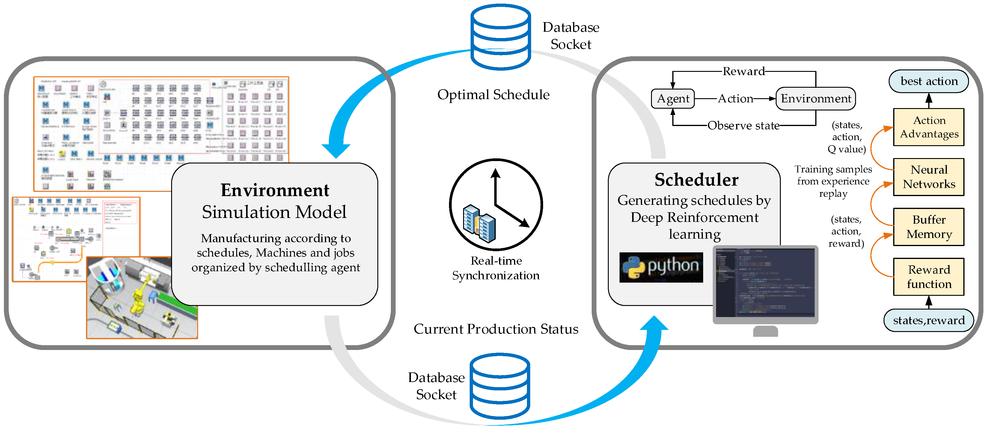
In this section we verify the effectiveness of the proposed real-time scheduling decision method based on MTMARL. Based on the model established in Section 2, the scheduling environment was developed using digital factory simulation software. The reinforcement learning training framework was developed in Python 3.8 according to Algorithm 1. The Socket communication mode was used for the interaction between the agent and the simulation environment to achieve performance training of the agent, as shown in Figure 6. Here, the Python development environment served as the server, and the scheduling simulation environment served as the client. As the digital factory simulation software can directly handle the data collection and command control in the workshop, this integrated interaction method improves the applicability of solving practical problems. The scheduling decision performance was studied throughout the simulation process by changing the number of cells, machines, and jobs, and the process planning data of jobs.

5.1. Parameters Descriptions

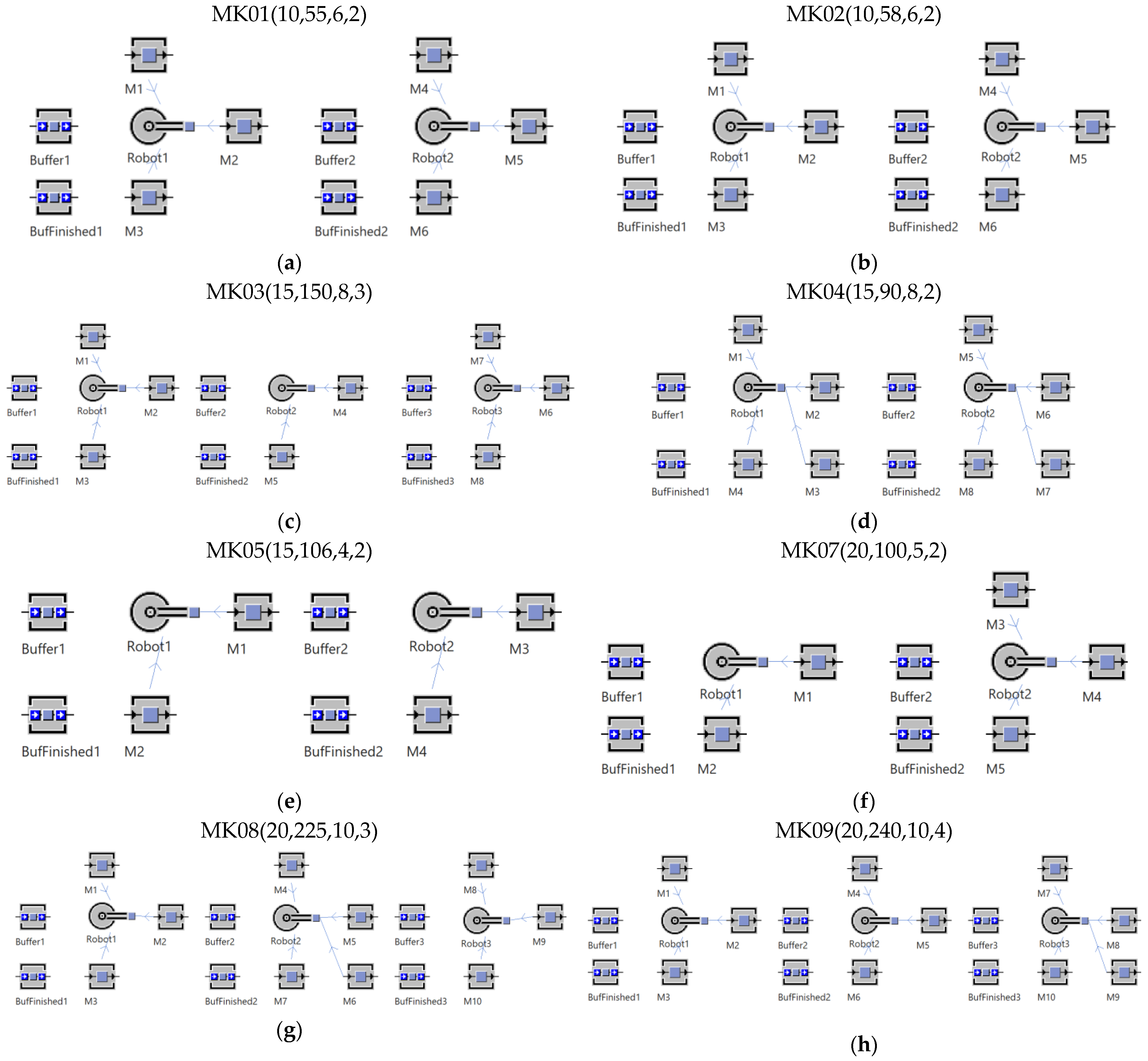
Due to the particularity of the scheduling problem proposed in this paper, there were no standard examples to support the experimental analysis. Therefore, in order to obtain data related to the FJSP-DP, the required simulation examples were randomly generated based on the data of MK01–MK10 examples provided by Brandimarte, which are standard examples of FJSP. In the example, the due time of job i is set to D i = α   j = 1 n i t ¯ ij , that is, the cumulative average processing time of all operations on the job.   α is a random coefficient between 1 and 2. It indicates the tightness of delivery date. For examples on different scales, the number of robots is 2–5 and the number of machines supervised by each robot at the same time conforms to the uniform distribution U [2–4]. The time for the robot to perform loading and unloading activities is related to the relative angular displacement of the robot base and the machine. In combination with the directed graph model of the process planning in Figure 2, U [2–5] node operations and the corresponding virtual operations are randomly generated. The number of operations and the processing time of the job are consistent with operations in the standard example, thus initializing the adjacency matrix of flexible process planning for each job. The above parameters are shown in Table 2.
The number of jobs and resources and the environmental layout of each calculation example based on the parameters in Table 2 are shown in Figure 7. For example, MK05 (15,106,4,2) represents the scheduling environment generated by MK05, which contains 15 jobs, 106 operations, and 4 machines divided into 2 work cells and 2 robots.
The pseudo-code development training algorithm is based on Section 4.5. The values of all hyperparameters of the algorithm were determined according to the size of the FJSP-DP example and the adjustment of the training process. The list of hyperparameters with their values is shown in Table 3.

5.2. Analysis of Results

5.2.1. Scheduling Process Data

The designed reinforcement learning scheduling framework interacts with the scheduling environment in each example. Obtain global state information through local observations. The state data of production scheduling were collected in the interaction process, so as to objectively evaluate the correlations between state characteristics. In this paper, the results obtained from MK01 were used for correlation analysis. In this example environment (shown in Figure 7a), there are two robots; each robot is responsible for supervising 3 machines, the number of jobs is 10, and the number of operations is 55. Figure 8a shows the change trend of state characteristic values with the decision time steps. According to the curve of the change trend, the state characteristics related to resources, including the average utilization rate of machines, the standard deviation of work cell utilization rate, and the average utilization rate of robots and its standard deviation, can quickly reach a stable numerical range as the number of decision steps increases. It can also be seen from the figure that after the trend stabilizes, the utilization rate of machines and robots is relatively close, which is about 60%. First, the utilization rate of the machine indirectly reflects the utilization rate of the work cell, which can be verified by Formula (29). Second, the utilization rate of the robot is restricted by tasks and resources in the work cell. The utilization rate of the robot is related to the work cell, which can be verified by the standard deviation curve of the utilization rate in Figure 8a. Therefore, the average utilization ratio of machines and robots is close. At the same time, the standard deviation of work cell and robot utilization rates is maintained around 10%, indicating that the load of each robot, work cell, and processing task are relatively balanced, effectively reflecting the scheduling objective of Formula (3) to minimize the workload difference among all robots.
On the other hand, the states related to the job task basically show a gradual linear increasing trend until the value becomes 1. We found that the estimated rate of tardiness changed earlier than the actual rate, and the trends were highly correlated, which shows that the method of calculating the estimated tardiness rate can effectively predict tardiness in advance and provide more accurate state parameters for the effective selection of corresponding scheduling rules. The correlation between state characteristics is shown in Figure 8b. Among them, the average completion rate, estimated tardiness rate, and actual tardiness rate related to the job show high correlation of 0.81, 0.85, and 0.94, respectively, because the process of calculating them is related to the number of completed job operations. At the same time, the average utilization rate of the machine is also highly correlated with the estimated tardiness of the job, because these are the main influencing factors in the reward design. Therefore, when the agent makes scheduling decisions, it will obtain greater rewards if it chooses jobs with large tardiness and low utilization, which makes the agent pay more attention to this selection policy. This mechanism is ultimately reflected in the correlation of state characteristics. The correlation between other state features is low, which shows that having state features with low coupling is more conducive to the effective learning of agents.
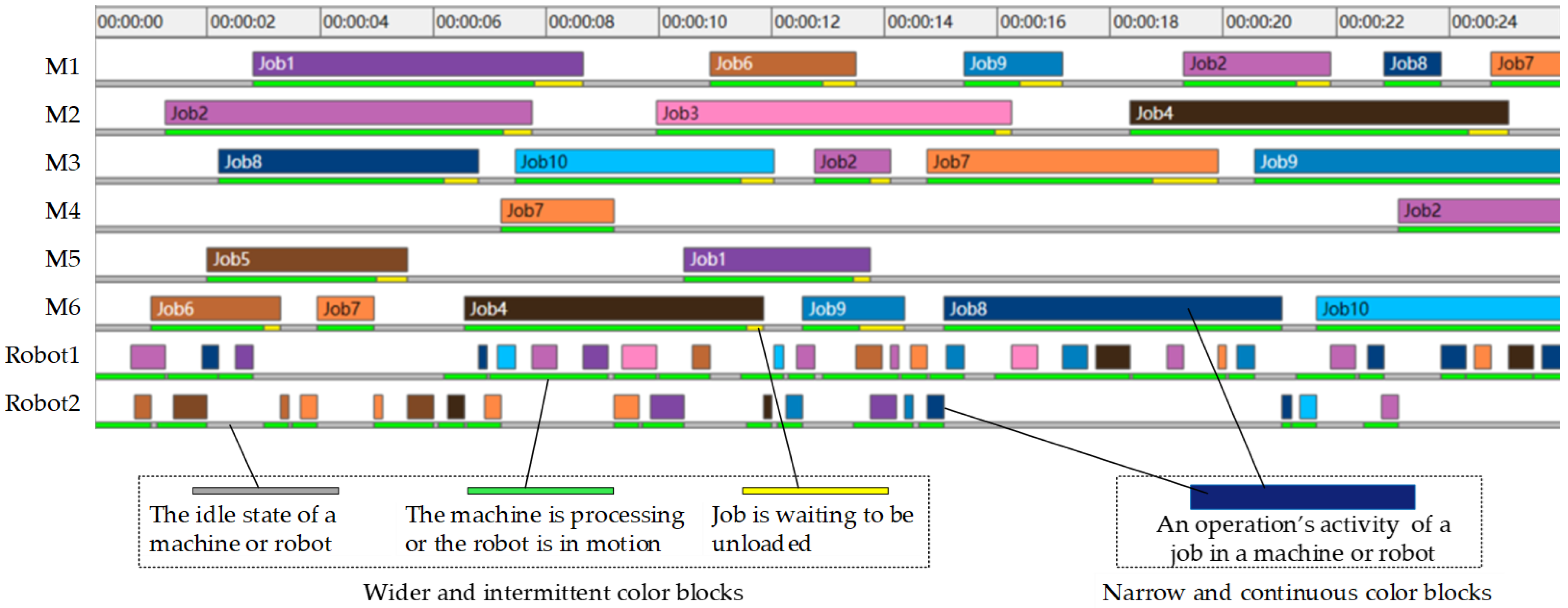
In addition, a Gantt chart of scheduling at each time was continuously generated in the process of real-time interaction between the scheduling environment and the agent. This real-time scheduling chart for the MK01 example environment is shown in Figure 9. In this Gantt chart, there are two kinds of color blocks. (1) Wider and intermittent color blocks. One block represents one operation of a certain job. One color represents one job. The length of the color block indicates the time of processing, loading, or unloading. The sequence of each job on the machine or robot is displayed by the order of the corresponding color blocks on the time axis. (2) Narrow and continuous color blocks. There are three colors in total, namely gray, green, and yellow. Among them, gray indicates that the machine or robot is in an idle state, green indicates that the machine is processing or the robot is in motion, and yellow indicates that the job on the machine has been processed and is waiting to be unloaded. The length of the color blocks indicates the duration of each state. It can be found that the robot has loaded and unloaded each job, and the machine has completed the processing of the job, and various constraints have been met in the scheduling model. The Gantt chart shows that the designed scheduling environment and reinforcement learning real-time scheduling method are suitable for solving the scheduling problem proposed in this paper.

5.2.2. Global Reward Convergence

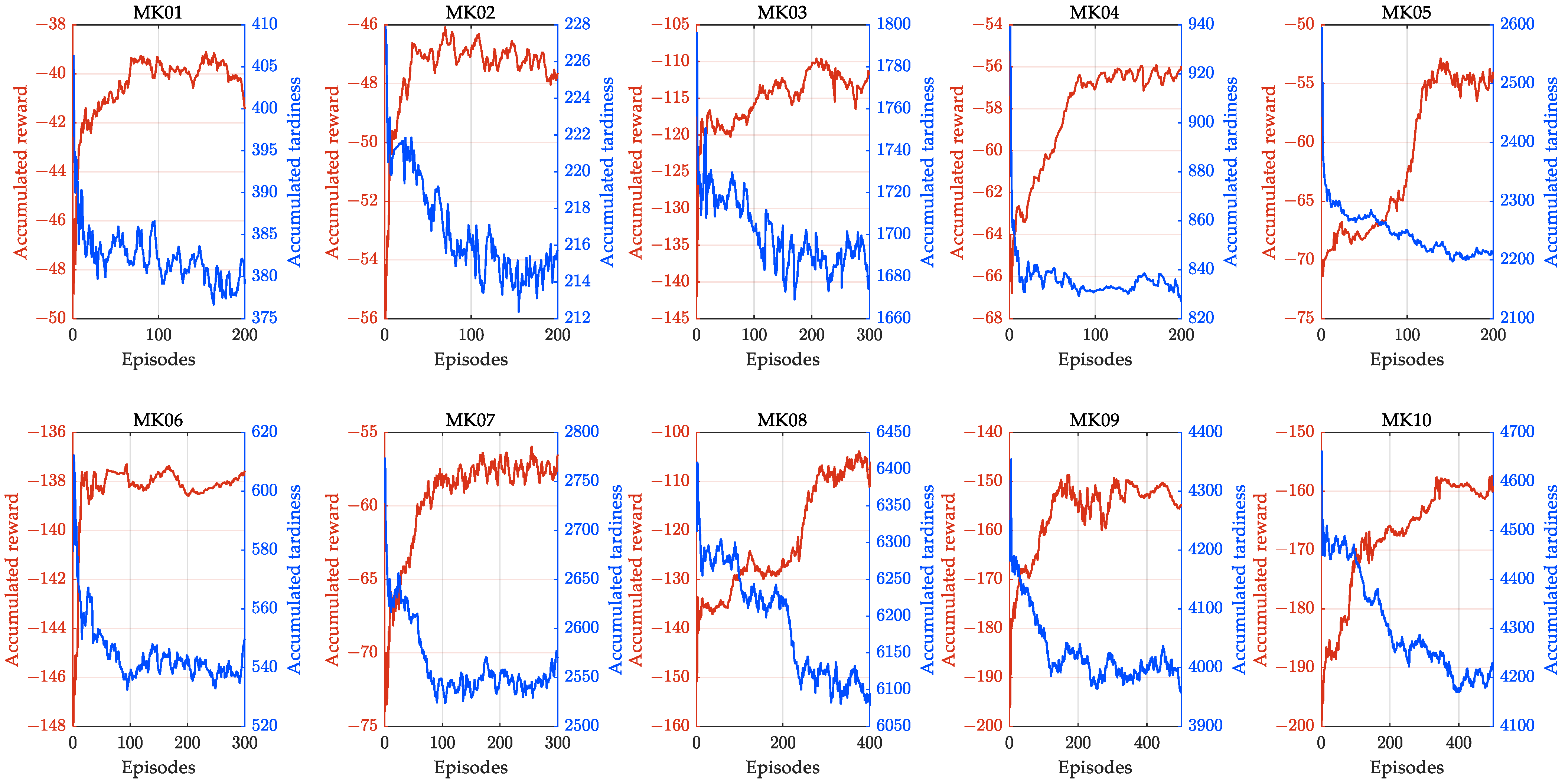
In order to further analyze the effectiveness of the proposed multi-task multi-agent reinforcement learning algorithm to solve the FJSP-DP problem, the convergence performance of the 10 groups of data derived from MK01–MK10 was analyzed. Different episodes were selected according to the size of the example. Figure 10 shows the global reward convergence of the proposed algorithm when solving scheduling problems of different scales. The red line in the figure is the convergence curve of the global reward function. It can be seen that with increased training rounds, the global reward function value gradually converges to a certain value.
The due time for the scheduling objective corresponding to the global reward is shown in the figure with a blue line. The delay time is inversely proportional to the overall reward, which is consistent with the trend reflected in the reward design. In the training process, it is obvious that the number of turns required to achieve convergence is related to the number of operations. However, it can be found in the figure that the number of rounds required is not too large, and the algorithm can converge to a relatively stable state, indicating that the convergence speed of the proposed algorithm is fast. In general, the scheduling agent learns appropriate scheduling rules according to changes in the production status, which improves the adaptability of FJSP-DP.

5.2.3. Local Reward Convergence

In order to analyze the performance of each agent when executing multi-task decisions, the convergence performance of local reward for each decision task was analyzed based on the FJSP-DP scheduling example using MK10, whose environment layout as shown in Figure 7a. Figure 11 shows the local reward convergence of each agent executing its own scheduling decision task in this example. For each decision task of each agent, its corresponding local reward function curve was drawn. There are two obvious trends in the figure. First, it can be seen that all agents were able to complete their associated tasks and maximize the specified reward function. Second, the proposed algorithm has a fast convergence rate. For most agents, the reward function for most tasks will converge when there are fewer than 100 episodes. Moreover, the stability of local reward convergence is better.
As the total number of operations is relatively large compared with the available processing resources, there is high competition between agents when selecting work cells to obtain the available processing resources. Therefore, the agents must share resources. This problem is crucial, because each agent selects the action corresponding to the task according to its own observation. It also implies that all agents in the scheduling decision system achieve balance in some way. The scheduling decision in the cell not only promotes each agent to select appropriate processing resources through global evaluation, but also stimulates the agent to complete the selection of jobs and machines in the cell through the local evaluation. Through training, the reward function converges, and the scheduling goal approaches the optimal value.

6. Conclusions and Prospects

In this paper, a mixed integer programming scheduling model is established to solve the dual resource FJSP problem with robots as well as flexible process planning. The scheduling decision task and dynamic process planning process are defined from the perspective of real-time scheduling. The scheduling task is decomposed into three decision tasks: job sequencing, machine selection, and process planning. In order to realize real-time scheduling decisions, a MTMARL framework based on centralized training and decentralized execution is proposed. The robot acts as an agent and interacts with the scheduling environment. In the process of centralized training, the value network is used to train and optimize the policy network of each agent to achieve cooperation among multiple agents. The policy network is constructed of three neural network layers: the expert layer composed of DDQN, the tower layer composed of neural networks, and the gate layer for entering the attention mechanism. The gate control layer is used to solve the information sharing of decision tasks. In the process of decentralized implementation, each agent completes three scheduling decision tasks for the corresponding work cell through its local observation according to the trained policy network. The state, action, and reward functions for reinforcement learning training in the context of the scheduling problem were designed, and the training algorithm was developed. Finally, the scheduling simulation environment was derived from international standard examples, and an example experiment was carried out. The results were discussed from the four aspects of state feature correlation, scheduling results, and global and local reward convergence of the algorithm. The results show that the proposed method can effectively solve the FJSP-DP. Meanwhile, the proposed MTMARL framework is conducive to the realization of real-time scheduling decisions with self-organization, self-learning, and self-optimization.
At present, this study has some limitations. In the MTMARL framework, the feature of the gate layer neural network for multi-task coordination is designed subjectively. This may lead to insufficient discrimination of the specificity for multi-task. To make up for this shortcoming, an automatic feature extraction method can be added to the framework to improve the overall performance of the algorithm. In addition, this framework is based on the mode of centralized training and decentralized execution. Although it effectively solves the real-time scheduling of FJSP-DP, we think that it may not be a multi-tasking system in the strict sense. This shortcoming can be addressed by combining the latest multi-task reinforcement learning, such as IMPALA (Importance-Weighted Actor-Learner Architectures). In addition, future research should consider logistical factors between work cells, such as AGV, and expand the adaptability of scheduling models and methods.

Author Contributions

Conceptualization, X.Z. and J.G.; data curation, X.Z.; investigation, X.Z. and J.X.; methodology, X.Z. and J.G.; project administration, J.X. and Y.W.; resources and software, J.X. and Z.X.; funding acquisition, Z.X.; writing—original draft, X.Z.; writing—review and editing, X.Z. and J.G. All authors have read and agreed to the published version of the manuscript.

Funding

This research was funded by the National Natural Science Foundation of China (Grant No. 61772160) and Heilongjiang Province Applied Technology Research and Development Plan, (Grant No. GA20A401).

Data Availability Statement

Not applicable.

Acknowledgments

The authors are grateful to the editor and reviewers for their constructive comments and suggestions, which have improved this paper.

Conflicts of Interest

The authors declare no conflict of interest.

References

  1. Bouazza, W.; Sallez, Y.; Beldjilali, B. A distributed approach solving partially flexible job-shop scheduling problem with a Q-learning effect. IFAC Pap. 2017, 50, 15890–15895. [Google Scholar] [CrossRef]
  2. Chang, J.; Yu, D.; Hu, Y.; He, W.; Yu, H. Deep Reinforcement Learning for Dynamic Flexible Job Shop Scheduling with Random Job Arrival. Processes 2022, 10, 760. [Google Scholar] [CrossRef]
  3. Lu, Y.; Xu, X.; Wang, L. Smart manufacturing process and system automation–a critical review of the standards and envisioned scenarios. J. Manuf. Syst. 2020, 56, 312–325. [Google Scholar] [CrossRef]
  4. Wang, S.; Wan, J.; Li, D.; Zhang, C. Implementing smart factory of industrie 4.0: An outlook. Int. J. Distrib. Sens. N. 2016, 12, 3159805. [Google Scholar] [CrossRef] [Green Version]
  5. Arents, J.; Greitans, M. Smart Industrial Robot Control Trends, Challenges and Opportunities within Manufacturing. Appl. Sci. 2022, 12, 937. [Google Scholar] [CrossRef]
  6. ElMaraghy, H.; Patel, V.; Ben Abdallah, I. Scheduling of manufacturing systems under dual-resource constraints using genetic algorithms. J. Manuf. Syst. 2000, 19, 186–201. [Google Scholar] [CrossRef]
  7. Li, X.; Gao, L. Review for Flexible Job Shop Scheduling; Engineering Applications of Computational Methods; Springer: Berlin/Heidelberg, Germany, 2020; pp. 17–45. [Google Scholar]
  8. Brucker, P.; Schlie, R. Job-shop scheduling with multi-purpose machines. Computing 1990, 45, 369–375. [Google Scholar] [CrossRef]
  9. Chaudhry, I.A.; Khan, A.A. A research survey: Review of flexible job shop scheduling techniques. Int. Trans. Oper. Res. 2016, 23, 551–591. [Google Scholar] [CrossRef]
  10. Xie, J.; Gao, L.; Peng, K.; Li, X.; Li, H. Review on flexible job shop scheduling. IET Collab. Intell. Manuf. 2019, 1, 67–77. [Google Scholar] [CrossRef]
  11. Gao, K.; Cao, Z.; Zhang, L.; Chen, Z.; Han, Y.; Pan, Q. A review on swarm intelligence and evolutionary algorithms for solving flexible job shop scheduling problems. IEEE/CAA J. Autom. Sin. 2019, 6, 904–916. [Google Scholar] [CrossRef]
  12. Zhang, X.; Liao, Z.X.; Ma, L.C.; Yao, J. Hierarchical multistrategy genetic algorithm for integrated process planning and scheduling. J. Intell. Manuf. 2020, 33, 223–246. [Google Scholar] [CrossRef]
  13. Lin, C.S.; Li, P.Y.; Wei, J.M.; Wu, M.C. Integration of process planning and scheduling for distributed flexible job shops. Comput. Oper. Res. 2020, 124, 105053. [Google Scholar] [CrossRef]
  14. Özgüven, C.; Özbakır, L.; Yavuz, Y. Mathematical models for job-shop scheduling problems with routing and process plan flexibility. Appl. Math. Model. 2010, 34, 1539–1548. [Google Scholar] [CrossRef]
  15. Phanden, R.K.; Jain, A.; Verma, R. Integration of process planning and scheduling: A state-of-the-art review. Int. J. Comput. Integr. Manuf. 2011, 24, 517–534. [Google Scholar] [CrossRef]
  16. Brucker, P.; Burke, E.K.; Groenemeyer, S. A branch and bound algorithm for the cyclic job-shop problem with transportation. Comput. Oper. Res. 2012, 39, 3200–3214. [Google Scholar] [CrossRef]
  17. Fatemi-Anaraki, S.; Tavakkoli-Moghaddam, R.; Foumani, M.; Vahedi-Nouri, B. Scheduling of Multi-Robot Job Shop Systems in Dynamic Environments: Mixed-Integer Linear Programming and Constraint Programming Approaches. Omega 2023, 115, 102770. [Google Scholar] [CrossRef]
  18. Ham, A. Transfer-robot task scheduling in flexible job shop. J. Intell. Manuf. 2020, 31, 1783–1793. [Google Scholar] [CrossRef]
  19. Vital-Soto, A.; Azab, A.; Baki, M.F. Mathematical modeling and a hybridized bacterial foraging optimization algorithm for the flexible job-shop scheduling problem with sequencing flexibility. J. Manuf. Syst. 2020, 54, 74–93. [Google Scholar] [CrossRef]
  20. Wu, X.; Peng, J.; Xiao, X.; Wu, S. An effective approach for the dual-resource flexible job shop scheduling problem considering loading and unloading. J. Intell. Manuf. 2020, 32, 707–728. [Google Scholar] [CrossRef]
  21. He, Z.; Tang, B.; Luan, F. An Improved African Vulture Optimization Algorithm for Dual-Resource Constrained Multi-Objective Flexible Job Shop Scheduling Problems. Sensors 2023, 23, 90. [Google Scholar] [CrossRef]
  22. Jiang, T.; Zhu, H.; Gu, J.; Liu, L.; Song, H. A discrete animal migration algorithm for dual-resource constrained energy-saving flexible job shop scheduling problem. J. Intell. Fuzzy Syst. 2022, 42, 3431–3444. [Google Scholar] [CrossRef]
  23. Hongyu, L.; Xiuli, W. A survival duration-guided NSGA-III for sustainable flexible job shop scheduling problem considering dual resources. IET Collab. Intell. Manuf. 2021, 3, 119–130. [Google Scholar] [CrossRef]
  24. Akbar, M.; Irohara, T. Scheduling for sustainable manufacturing: A review. J. Clean Prod. 2018, 205, 866–883. [Google Scholar] [CrossRef]
  25. Costa, A.; Cappadonna, F.A.; Fichera, S. A hybrid genetic algorithm for job sequencing and worker allocation in parallel unrelated machines with sequence-dependent setup times. Int. J. Adv. Manuf. Technol. 2013, 69, 2799–2817. [Google Scholar] [CrossRef]
  26. Akbar, M.; Irohara, T. Dual Resource Constrained Scheduling Considering Operator Working Modes and Moving in Identical Parallel Machines Using a Permutation-Based Genetic Algorithm. In Proceedings of the IFIP WG 5.7 International Conference on Advances in Production Management Systems (APMS), Seoul, Republic of Korea, 26–30 August 2018; pp. 464–472. [Google Scholar]
  27. Akbar, M.; Irohara, T. A social-conscious scheduling model of dual resources constrained identical parallel machine to minimize makespan and operator workload balance. In Proceedings of the Asia Pacific Industrial Engineering & Management System Conference, Auckland, New Zealand, 2–5 December 2018. [Google Scholar]
  28. Akbar, M.; Irohara, T. Metaheuristics for the multi-task simultaneous supervision dual resource-constrained scheduling problem. Eng. Appl. Artif. Intell. 2020, 96, 104004. [Google Scholar] [CrossRef]
  29. Qin, Z.; Lu, Y. Self-organizing manufacturing network: A paradigm towards smart manufacturing in mass personalization. J. Manuf. Syst. 2021, 60, 35–47. [Google Scholar] [CrossRef]
  30. Unterberger, E.; Hofmann, U.; Min, S.; Glasschröder, J.; Reinhart, G. Modeling of an energy-flexible production control with SysML. Procedia CIRP 2018, 72, 432–437. [Google Scholar] [CrossRef]
  31. Yue, H.; Xing, K.; Hu, H.; Wu, W.; Su, H. Supervisory control of deadlock-prone production systems with routing flexibility and unreliable resources. IEEE Trans. Syst. Man Cybern. Syst. 2019, 50, 3528–3540. [Google Scholar] [CrossRef]
  32. Assid, M.; Gharbi, A.; Hajji, A. Production control of failure-prone manufacturing-remanufacturing systems using mixed dedicated and shared facilities. Int. J. Prod. Econ. 2020, 224, 107549. [Google Scholar] [CrossRef]
  33. Ma, Y.-M.; Qiao, F.; Chen, X.; Tian, K.; Wu, X.-H. Dynamic scheduling approach based on SVM for semiconductor production line. Comput. Integr. Manuf. Syst. 2015, 21, 733–739. [Google Scholar]
  34. Azab, E.; Nafea, M.; Shihata, L.A.; Mashaly, M. A Machine-Learning-Assisted Simulation Approach for Incorporating Predictive Maintenance in Dynamic Flow-Shop Scheduling. Appl. Sci. Basel 2021, 11, 11725. [Google Scholar] [CrossRef]
  35. Xiong, W.; Fu, D. A new immune multi-Agent system for the flexible job shop scheduling problem. J. Intell. Manuf. 2018, 29, 857–873. [Google Scholar] [CrossRef]
  36. Luo, S. Dynamic scheduling for flexible job shop with new job insertions by deep reinforcement learning. Appl. Soft. Comput. 2020, 91, 106208. [Google Scholar] [CrossRef]
  37. Han, B.; Yang, J. A deep reinforcement learning based solution for flexible job shop scheduling problem. Int. J. Simul. Model. 2021, 20, 375–386. [Google Scholar] [CrossRef]
  38. Luo, S.; Zhang, L.; Fan, Y. Real-Time Scheduling for Dynamic Partial-No-Wait Multiobjective Flexible Job Shop by Deep Reinforcement Learning. IEEE Trans. Autom. Sci. Eng. 2021, 19, 3020–3038. [Google Scholar] [CrossRef]
  39. Liu, R.; Piplani, R.; Toro, C. Deep reinforcement learning for dynamic scheduling of a flexible job shop. Int. J. Prod. Res. 2022, 60, 4049–4069. [Google Scholar] [CrossRef]
  40. Johnson, D.; Chen, G.; Lu, Y. Multi-Agent Reinforcement Learning for Real-Time Dynamic Production Scheduling in a Robot Assembly Cell. IEEE Robot Autom. Let. 2022, 7, 7684–7691. [Google Scholar] [CrossRef]
  41. Lei, K.; Guo, P.; Zhao, W.C.; Wang, Y.; Qian, L.M.; Meng, X.Y.; Tang, L.S. A multi-action deep reinforcement learning framework for flexible Job-shop scheduling problem. Expert Syst. Appl. 2022, 205, 117796. [Google Scholar] [CrossRef]
  42. Jiang, Y.; Cao, Z.; Zhang, J. Learning to Solve 3-D Bin Packing Problem via Deep Reinforcement Learning and Constraint Programming. IEEE T. Cybern. 2021, 1–12. [Google Scholar] [CrossRef]
  43. Omidshafiei, S.; Pazis, J.; Amato, C.; How, J.P.; Vian, J. Deep Decentralized Multi-task Multi-Agent Reinforcement Learning under Partial Observability. In Proceedings of the 34th International Conference on Machine Learning, Sydney, Australia, 6–11 August 2017. [Google Scholar]
  44. Liu, X.; Zhang, G. A flexible job shop online scheduling approach based on process-tree. J. Theor. Appl. Inf. Technol. 2012, 44, 259–264. [Google Scholar]
  45. Mnih, V.; Kavukcuoglu, K.; Silver, D.; Graves, A.; Antonoglou, I.; Wierstra, D.; Riedmiller, M. Playing atari with deep reinforcement learning. arXiv 2013, arXiv:1312.5602. [Google Scholar]
  46. Mnih, V.; Kavukcuoglu, K.; Silver, D.; Rusu, A.A.; Veness, J.; Bellemare, M.G.; Graves, A.; Riedmiller, M.; Fidjeland, A.K.; Ostrovski, G. Human-level control through deep reinforcement learning. Nature 2015, 518, 529–533. [Google Scholar] [CrossRef] [PubMed]
  47. Van Hasselt, H.; Guez, A.; Silver, D. Deep reinforcement learning with double q-learning. In AAAI Conference on Artificial Intelligence; AAAI: Palo Alto, CA, USA, 2016; pp. 2094–2100. [Google Scholar]
  48. Panwalkar, S.S.; Iskander, W. A Survey of Scheduling Rules. Oper. Res. 1977, 25, 45–61. [Google Scholar] [CrossRef]
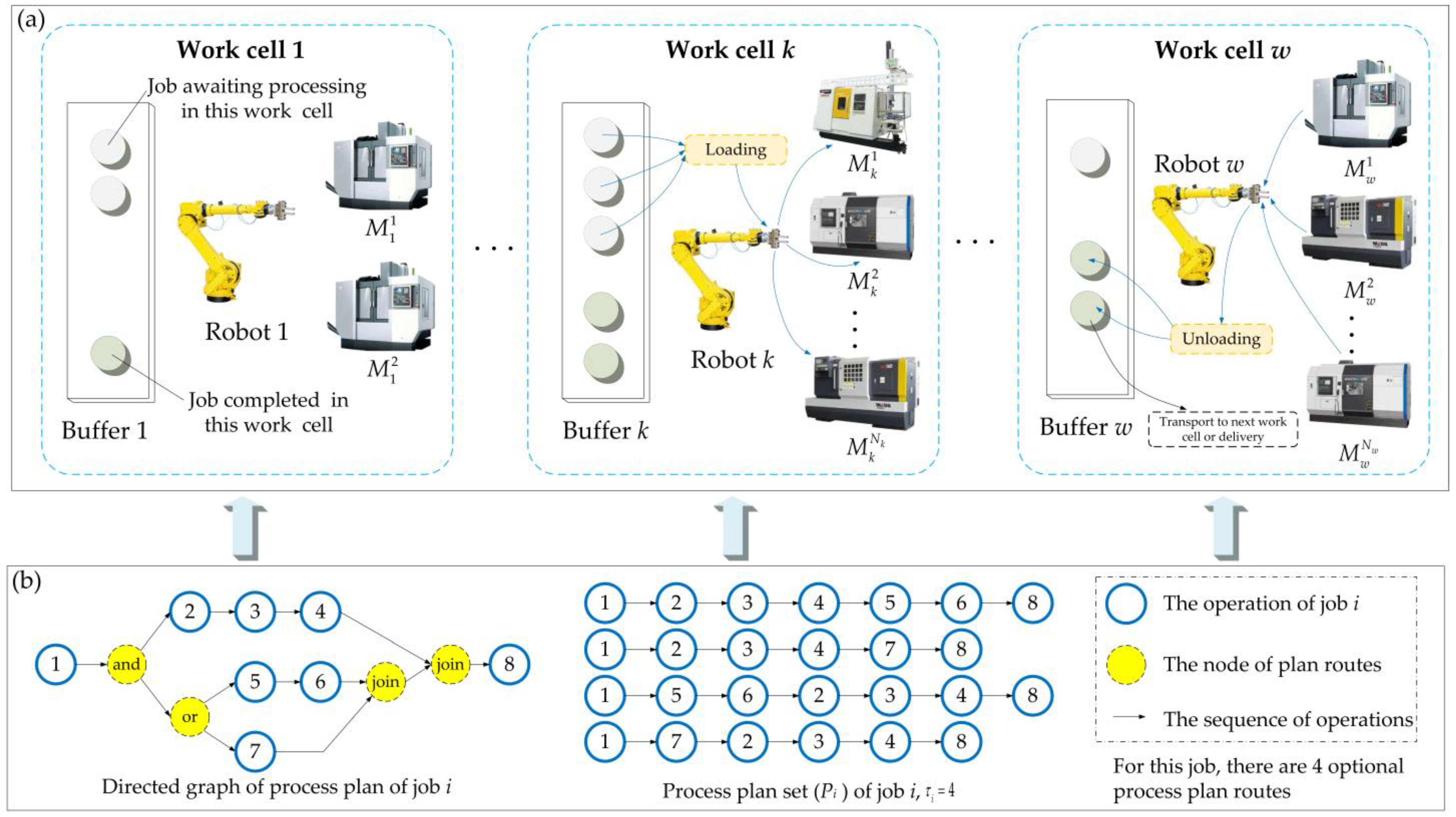
Figure 1. Composition of workshop: (a) schematic diagram of w work cells; (b) schematic diagram of process planning for a job.
Processes 11 00267 g001
Figure 2. Dynamic updating diagram of process planning based on process tree.
Processes 11 00267 g002
Figure 3. Execution process of scheduling decision.
Processes 11 00267 g003
Figure 4. Principle of DDQN for solving scheduling.
Processes 11 00267 g004
Figure 5. Scheduling decision framework.
Processes 11 00267 g005
Figure 6. Real-time interaction of agent with scheduling environment.
Processes 11 00267 g006
Figure 7. Example scheduling environment layout diagrams.
Processes 11 00267 g007aProcesses 11 00267 g007b
Figure 8. (a) Change curve and (b) correlation analysis of global state characteristics.
Processes 11 00267 g008
Figure 9. Gantt chart of real-time scheduling of FJSP-DP (MK01).
Processes 11 00267 g009
Figure 10. Convergence curve of global reward and tardiness.
Processes 11 00267 g010
Figure 11. Convergence curve of local reward for each task of FJSP-DP (MK10).
Processes 11 00267 g011
Table 1. Rules for machine selection.
RuleDescriptionFormula
Dispatching rule 6Select machine with the lowest workload argmin h M k empty i = 1 n j = 1 O P i ( t ) X ijh T ijh 1
Dispatching rule 7Select machine with the longest waiting time argmax h M k empty ( t C T h ( t ) )
Dispatching rule 8Select machine that takes the least time to process the selected job argmin h M k empty X ijh T ijh
Table 2. Scheduling environment parameters.
ParameterValue
Number of robots2–5
Number of machines supervised by each robotU [2–4]
Number of node operations of the jobU [2–5]
Speed robot performs loading and unloading30°/time unit
Number of jobsSee standard example
Number of machinesSee standard example
Number of operationsSee standard example
Table 3. Neural network parameters and their values.
ParameterValue
Replay buffer size50,000
Minibatch64
Size of hidden layers in policy network3/64, 64, 1
Size of hidden layers in critic network3/64, 64, 12
Size of hidden layers in target policy network3/64, 64, 1
Size of hidden layers in target critic network3/64, 64, 12
Learning rate0.01
Discount factor0.95
Update rate of target network0.01
Episode200–500
Disclaimer/Publisher’s Note: The statements, opinions and data contained in all publications are solely those of the individual author(s) and contributor(s) and not of MDPI and/or the editor(s). MDPI and/or the editor(s) disclaim responsibility for any injury to people or property resulting from any ideas, methods, instructions or products referred to in the content.