An Advanced Multifidelity Multidisciplinary Design Analysis Optimization Toolkit for General Turbomachinery

Abstract

The MDAO framework has become an essential part of almost all fields, apart from mechanical, transportation, and aerospace industries, for efficient energy conversion or otherwise. It enables rapid iterative interaction among several engineering disciplines at various fidelities using automation tools for design improvement. An advanced framework from low to high fidelity is developed for ducted and unducted turbomachinery blade designs. The parametric blade geometry tool is a key feature which converts low-fidelity results into 3D blade shapes and can readily be used in high-fidelity multidisciplinary simulations as part of an optimization cycle. The geometry generator and physics solvers are connected to DAKOTA, an open-source optimizer with parallel computation capability. The entire cycle is automated and new design iterations are generated with input parameter variations controlled by DAKOTA. Single- and multi-objective genetic algorithm and gradient method-based optimization cases are demonstrated for various applications. B-splines are used to define smooth perturbation of parametric variables chordwise and spanwise of the blade. The ability to create parametric 3D blade shapes quickly from low-fidelity analyses with advanced control is demonstrated to be unique and enables a rapid 3D design cycle. Non-intuitive designs are feasible in this framework and designers can really benefit from parametric geometry manipulation. Optimization at each fidelity is realized through automation. As part of the multidisciplinary analysis, 3D structural analysis is also performed using the unidirectional fluid–structure interaction for a few cases with imported pressure loads from the 3D RANS solution. Examples of axial turbofans, compressor rotors, turbines, radial compressors, propellers, wind and hydrokinetic turbines are demonstrated to prove generality.

1. Introduction

Turbomachinery design is a highly iterative and complex multidisciplinary process. An efficient design depends on the best exploits and interactions among various disciplines for desired aerodynamic performance, structural integrity, manufacturability, lifecycle costs, product cycle time, and business model. The multifidelity multidisciplinary design analysis optimization (MDAO) approach is very useful in obtaining an optimized design while satisfying several constraints. Using this approach at the conceptual phase of a design cycle is important as the largest influence on the final product occurs at this stage and 3D design improvements can be achieved with feasible trade-offs before manufacturing the hardware. An integration framework is required for multidisciplinary optimization to manage and automate the interaction between various tools and disciplines, enabling concurrent analysis and automatic execution of multiple tools at various levels of fidelity, as explained by Panchenko et al. [1]. The framework must be robust to include various optimization strategies, the definition of a large design space, meaningful objective function definitions which are subject to various performance and geometrical constraints, must operate with minimal human interaction, and must be highly parallel to save computational time [2,3,4,5,6,7].

Ultimately, any optimization process requires human interference. Their design knowledge should guide the user in setting up the problem, defining objectives and constraints, in performing sensitivity analyses, combining different disciplines, interpreting results, and hence directing the optimizer to obtain the desired goal [7]. A sophisticated but simple-to-use parameterization of the data (geometrical or otherwise) is very crucial in the optimization process as it helps to reduce the number of design variables. Parametric sensitivity analysis provides insight into the degree of influence each design variable has over the performance and enables the designer to choose highly sensitive parameters [8,9,10]. After this step, various solvers are executed which compute all objectives and constraints that are relevant to the multidisciplinary design [7]. Some solvers are run sequentially, where the output of one solver is the input (partially) for another solver and can also be run in parallel if there is no data transfer between the solvers. To reduce the computational time, surrogate models are used to approximate the results of computationally expensive solvers and are trained during optimization [11,12]. Using the original solvers once more, the real optimum is obtained with the approximated optimum as a good initial guess. A pre-evaluation tool processes the output of the solvers and reduces the data to objectives and constraints with respective ranges if the output does not explicitly contain them [7]. Assessment of the objectives and constraints is carried out by the evaluator, which prepares the model for the optimizer.

Mathematical definition of objective function(s) should be meticulously formulated to take complete advantage of perturbations of design parameters and the goal to be achieved from the optimal design. Having a good database of iterations paves the way for future optimization challenges, and a baseline can be chosen from that dataset. The search mechanism in optimization schemes is the most important feature to reach an answer rapidly with less resources. Search mechanisms are utilized to find the optimum combination of design parameters and are classified as gradient-based or non-gradient-based [12]. The gradient-based method uses derivatives of response functions to find the improvement direction. Non-gradient-based methods largely use pattern search, genetic algorithms, the Tabu search algorithm [13,14], and nonlinear least squares [12]. Objective functions are minimized or maximized to obtain the desired optimum result. In the 3D blade optimization loop, the process can be CAD-free or CAD-based. One of the benefits of having the CAD-based (through a flexible interface) optimization process is geometrical accuracy as the translational errors are minimized and a minimum turn-around time is achieved [14]. However, CAD splines vary from tool to tool and hence, CAD-free methods are more widely used to manipulate geometry using smooth B-splines, Bezier curves, or NURBS [15,16,17,18,19,20]. Higher-order polynomials to create smooth surfaces by matching the slope of curves at the point of connection can be used to define the flow path. A smooth, supersonic, rectangular nozzle shape defined by two curves with their slopes matched at the throat was created to mitigate shock formation, as demonstrated by Bhide [21]. The fluid–thermal–structural interaction in supersonic nozzles is also demonstrated by Bhide et al. [22] using multiphysics framework in ANSYS [23] with the philosophy described here.

Several case studies are summarized here which use multifidelity multidisciplinary optimization at various stages of the design process. Cases with high-fidelity optimization of turbomachinery are described by Pierret et al. [24], Braembussche et al. [25], Grasel et al. [26], Demeulenare et al. [27,28], and in some recent papers [29,30]. Design researchers have also demonstrated multidisciplinary optimization connected to CAD [31] or otherwise looking at blockage and loss [13,14], adiabatic efficiency and pressure ratio [32,33,34,35], stall margin [36,37], minimal component weight [35,38], pressure loss and improved recovery coefficient [39,40], reduced mechanical stress [41,42,43,44,45], operating range extension [46], maximum power extraction [47,48], and device sizing [7]. Ease of manufacturability, low and high cycle fatigue-based constraints, performance improvements at various fidelities, and novel design exploration are some of the crucial goals to achieve. In addition to geometry manipulation and design optimization, improving the accuracy of physics and turbulence capture, especially in supersonic flows, is also important for multiphysics solutions, and is demonstrated by Bhide et al. [49,50,51]. Coupled multiphysics simulation can also be utilized in the exploration of novel conceptual engineering applications. Bhide [52] demonstrated the fluid–thermal–structural interaction of rectangular supersonic nozzles in retro-propulsion for a set of free-stream and operating conditions for the first time ever. Parallel computing is essential to drastically reduce the optimization cycle time and explore more designs rapidly before moving to expensive hardware development and testing phases. The DAKOTA framework is the basis for the MDAO toolkit detailed in this manuscript and is capable of several levels of parallel execution, as explained in the manual [12]. Asynchronous local parallelism is utilized in some optimization cases in this manuscript, where DAKOTA executes on a single processor, but launces a predefined batch of jobs concurrently and moves to the next batch. This method expedites the solution time of low- to medium-fidelity physics solver-based optimization cases.

The aim of this work is to demonstrate a comprehensive framework on multifidelity multidisciplinary design analysis optimization for ducted axial and radial turbomachines, and unducted high aspect ratio turbomachines such as propellers, wind and hydrokinetic turbines. In addition to traditional optimization, the framework also demonstrates advanced shape control using the curvature-driven meanline and smooth spanwise parametric variations using B-splines at low and high fidelity focused on flow physics. Optimization routines are automated at every fidelity to exploit the physics defined at these levels. The data transfer between physics solvers is consistent to facilitate robust fluid–structure interactions. The JEGA-based genetic algorithm and gradient methods are majorly used in these optimizations using DAKOTA.

2. Methodology

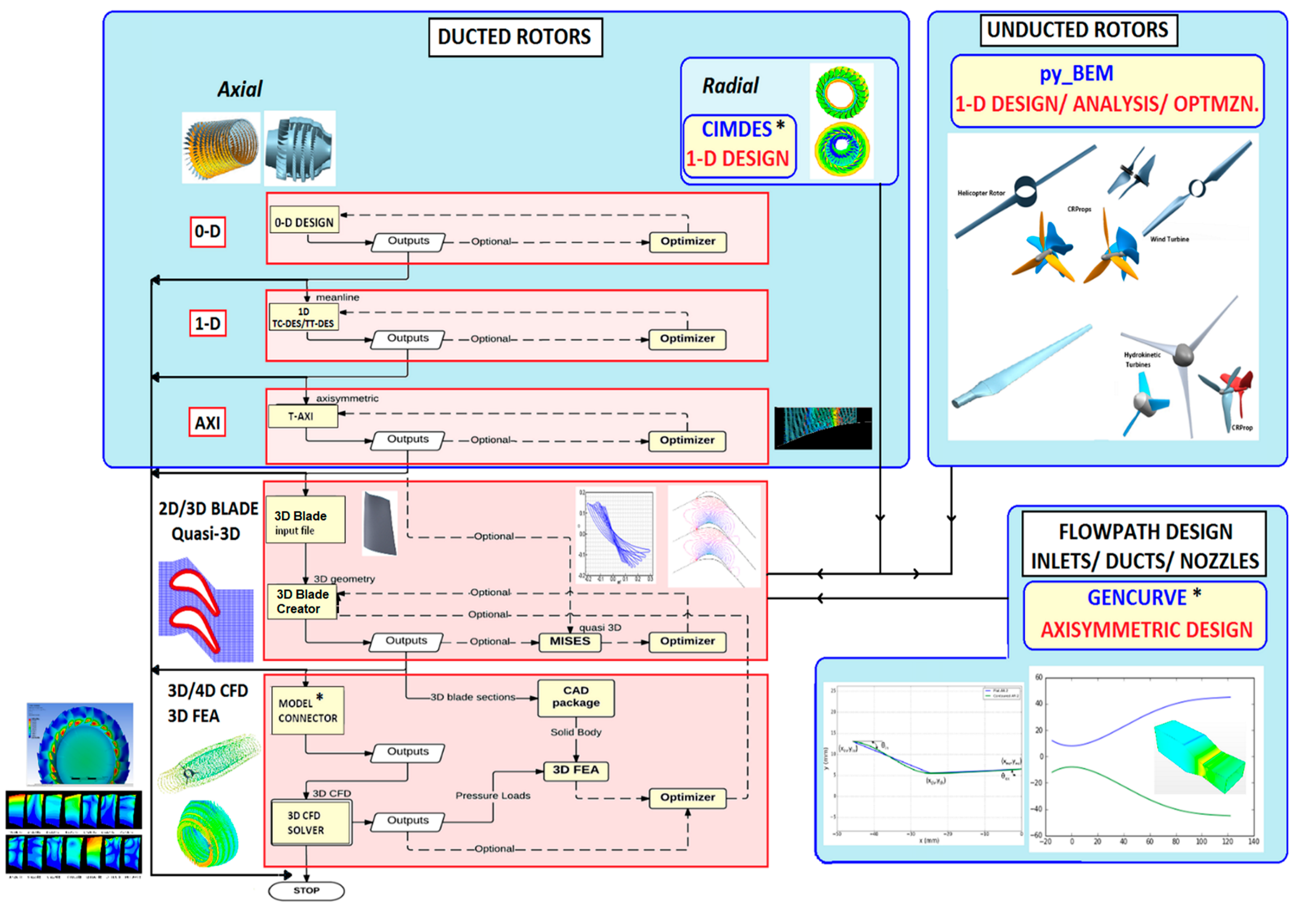
2.1. Overview

A multifidelity optimization process is required to obtain designs which are efficient while accounting for the 3D aeroelastic effects. Automation of the tool chain is the first step to obtain a robust optimization framework. This framework really tests the tools individually due to its exploratory nature, and appropriate checks and error captures need to be implemented. The parametric definition of the B-splines makes the geometry modification process quicker and easier and allows exploration of some novel concepts. All the Boolean operations are performed in CAD to obtain a water-tight solid. The geometry can be easily tied to any automation and optimization chain. DAKOTA provides a flexible, extensible interface between analysis codes and iterative systems analysis methods. It works in parallel with several optimization options and runs under Linux-, Unix-, and Linux-like environments (Windows with Cygwin). An automation system has been developed for geometry creation and mesh generation, and 3D CFD with post-processing of results, which could become objective function(s) for any design optimization. Figure 1 shows the 3D CFD optimization loop using DAKOTA, FINE/Turbo, and the geometry creator. A complete automation process for the multifidelity design analysis optimization framework is described in Figure 1, mainly developed for ducted rotors and general enough to be utilized for unducted rotors after replacing the 0D-1D-Axisymmetric part with BEMT or other similar low-fidelity tools. Each fidelity can be optimized before moving to the next level. Multidisciplinary analysis is also enabled for multi-objective optimization at high fidelity. The framework can handle axial and radial ducted turbomachinery along with unducted rotors such as propellers, wind and hydrokinetic turbines.

2.2. Design Variables and Constraints

Parameterization reduces the number of design variables needed in an optimization chain. Geometry parametrization is necessary in a shape optimization process and must be able to generate a large variety of physically realistic shapes with few design variables. It must be robust, such that a random perturbation of design variables should still provide a realistic blade, be generic enough to be applied to a large variety of problems and be able to integrate with any existing CAD system [7]. Smooth variation of parameters is integral to finding better optimums. Metal angles, LE, TE position of splitters, curved LE and TE, lean and sweep of blades, spanwise chord and stagger distribution, curvature-driven meanline-based airfoil, thickness, and flow path curves are some of the many design variables and constraints used in optimization challenges.

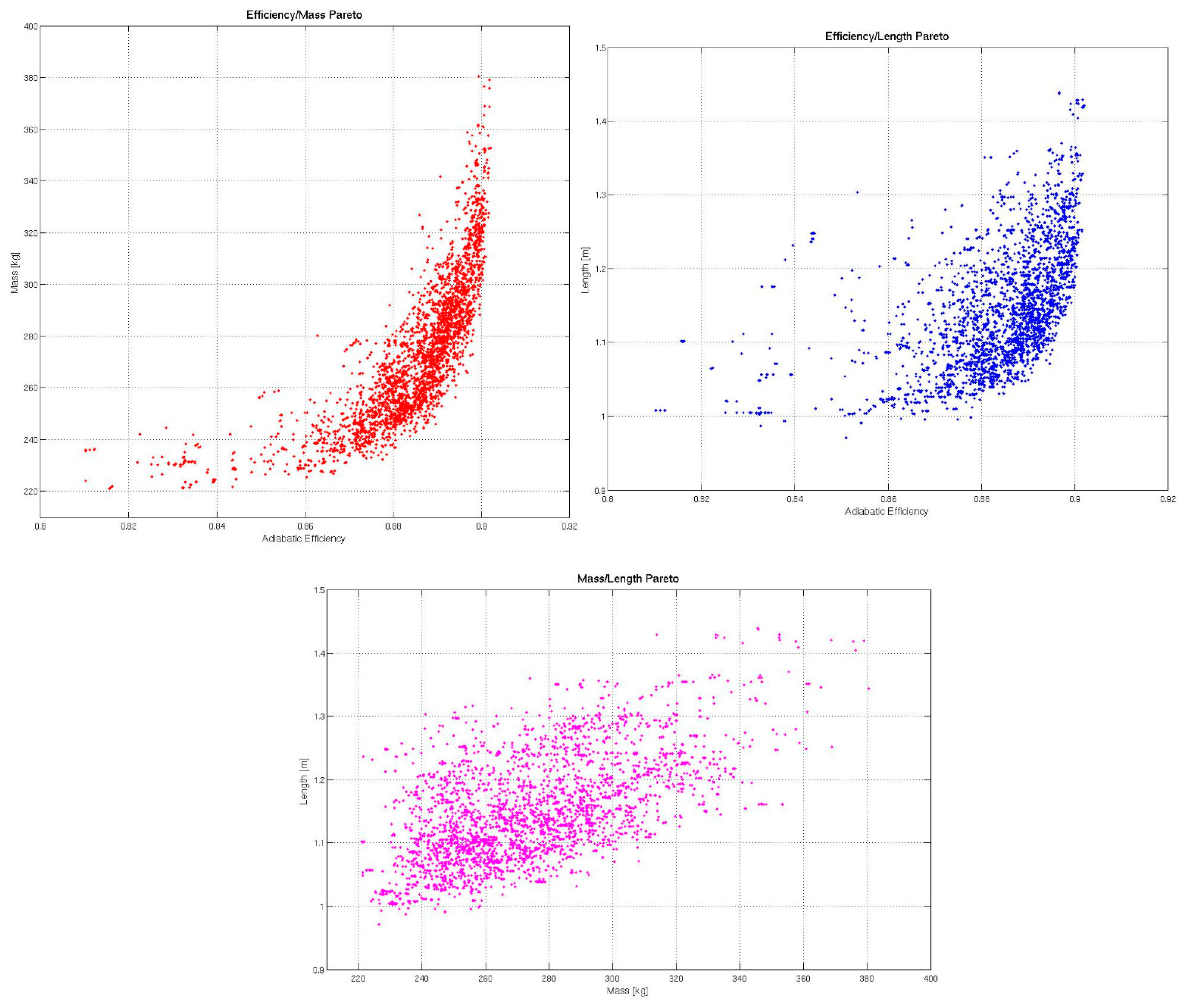
2.3. Objective Function and Pareto Front

The objective function (OF) is a measure of how well the aero-requirements are satisfied and whether the set performance goals have been achieved. Apart from aero-performance, other constraints such as the maximum stress level and manufacturability must also be satisfied. This results in an inequality and can be addressed by adding penalty terms to the OF, which increase when violation of the constraints occurs [25]. The relative importance of each term in the optimization procedure is given by the weight factor, which is multiplied to each term. Multi-objective functions can be plotted using pareto distributions to understand the optimizer’s direction and choose candidates to investigate further.

2.4. Search Algorithms

Non-gradient- and gradient-based search algorithms are the broad classification. The genetic algorithm is a non-gradient method based on the natural selection process and evolution in nature. An initial population is randomly generated in the design space. Each of these design points are evaluated. The best points are chosen, recombined, and mutated to create a new set of design points. The process is repeated until convergence criteria are satisfied. Single- and multi-objective genetic algorithms (SOGA, MOGA) from the John Eddy Genetic Algorithm (JEGA) library of DAKOTA [12] are used in the optimization.

2.5. MDAO Framework

Starting from a 0D analysis, the design process progressing to a 3D design is described here. Many of the tools which were created for ducted rotors are also used for unducted rotor design at mid-to-higher fidelity, with some assumptions and constraints. They also provide a basis for creating tools for unducted rotors by overcoming the constraints and fine-tuning the existing tools to make them general.

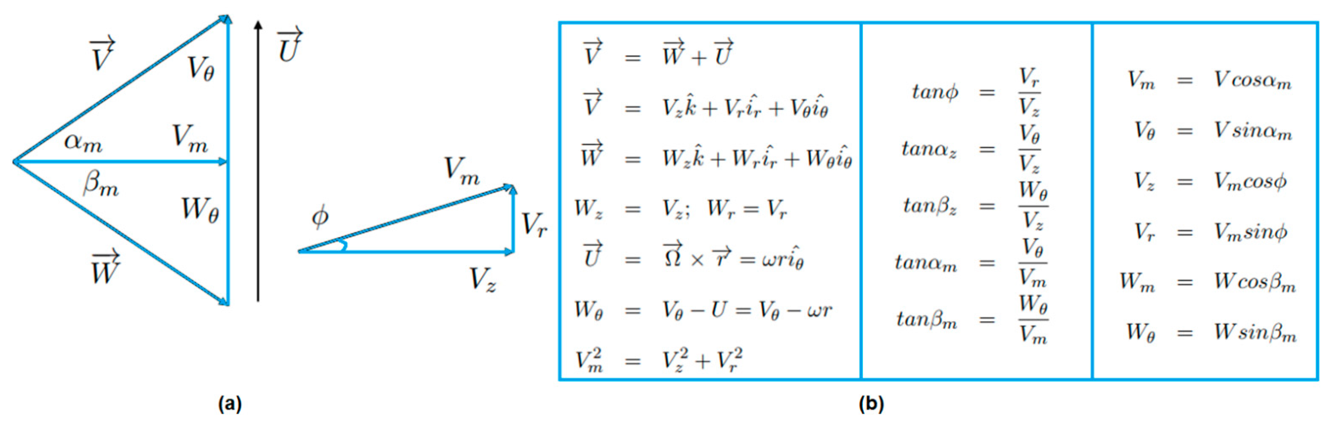
2.5.1. General Notation and Formalism

A general velocity triangle nomenclature is used, which can be applied for both ducted and unducted rotors, as shown in Figure 2. There is a distinction between meridional and axial velocity and the angle between them is defined as streamline slope, φ. For a meanline calculation, V_r = 0 and φ = 0 ⇒ V_m = V_z for axial machines, but it is not true when the hub slope becomes significant. The absolute and relative flow angles are shown in the figure. It also shows their relationship with each other and velocities established using trigonometry.

It is prudent to have a combined and general design tool for various ducted and unducted rotors, which include air and ship propellers, wind and tidal/hydrokinetic turbines, and helicopter rotors in vertical ascent/hover, adapting a few tools from the ducted rotor design environment in higher fidelity. A coordinate system and notation must be decided to keep consistency in the design and smooth information flow between fidelities. Blade rotation is positive in the 3D CFD solver for propellers/compressors and negative for turbines looking from the front.

2.5.2. Ducted Rotors: 0D Design

Isentropic relations are used to calculate the initial properties for any design before a 1D meanline design is initiated. It assumes efficiency and calculates the work done (ΔT_total) per stage for a multi-stage machine. It also calculates the inlet Mach number using an iterative solver based on the bisection method with a given radius ratio using Equation (1). Figure 3 shows an example case with input properties for a turbofan and the properties calculated. It also shows the variation of the equation with the Mach number and the solution for this case. Other isentropic properties can be calculated which are suitable for sizing the machine.

$$f\left(M\right)=\left(\frac{A_{inlet}{P}_0}{\dot{m}}\sqrt{\frac{\gamma }{R_{gas}{T}_0}}\right)M-{\left(1+\frac{\gamma -1}{2}{M}^2\right)}^{\frac{\gamma +1}{2\left(\gamma -1\right)}}=0$$

(1)

2.5.3. Ducted Rotors: 1D Meanline Design

Meanline solvers are used to obtain thermodynamic properties and aerodynamic parameters at several flow stations of the device. T-CDes and T-TDes of T-Axi suite of tools [53,54,55] are used for meanline designs for axial compressors and turbines. The authors also worked with Muppana [56] and Mishra [57] to create a meanline design tool for single- and multi-stage radial impellers. Free vortex or forced vortex laws can be used to create properties at hub and tip stations. Slip factor formulation is used for defining work performed for radial impellers, accounting for the Coriolis effect [58]. Vector triangles for the rotor can also be visualized and performance parameters can be varied to observe the effect of the preliminary design variations using T-Axi Blade, which is part of the T-Axi suite and is shown for an example turbofan rotor in Figure 4. It shows the rotor velocities at the inlet and exit for hub, midspan, and tip sections. The Smith chart shows the work and flow coefficients.

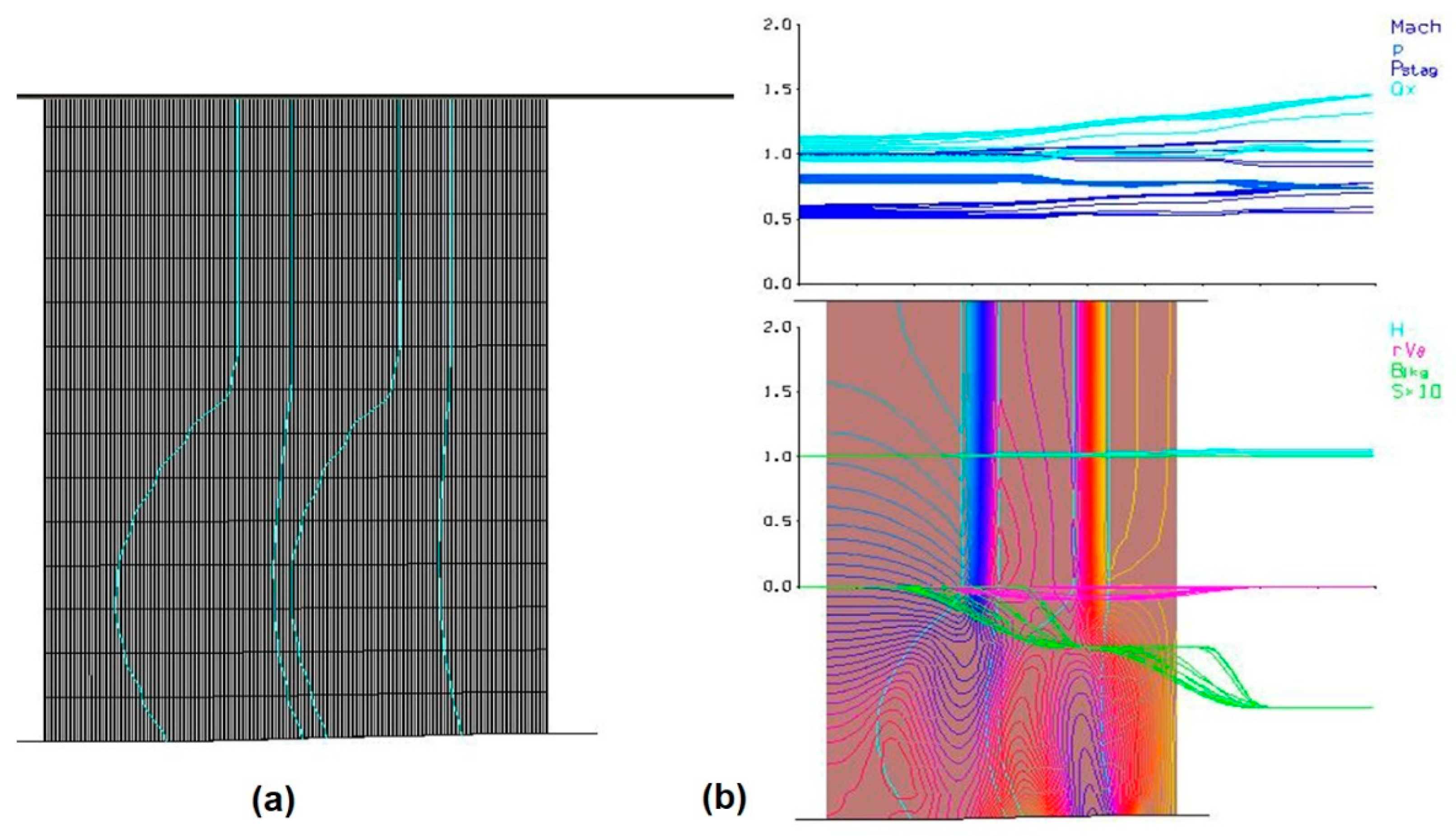
2.5.4. Ducted Rotors: Axisymmetric Design

An axisymmetric solver called T-Axi [53,54,55] is used to calculate spanwise properties of a device with loss models incorporated. It also generates 2D airfoil sections and is also used to create inputs for the 3D blade geometry generator. Figure 5 shows T-Axi runs of several examples, such as a transition duct between the combustor and axial turbine for a JetCat engine, a transonic fan showing property variation along the axis, 3D view of the single-stage fan, and initial design of a three-stage LPC and a multistage turbine with 3D view. Mach, static and stagnation pressure, blockage, angular momentum and entropy plots across the flowpath can be seen in the figure.

2.5.5. Ducted Rotors: Quasi-3D Design

MISES [59] is used to perform quasi-3D simulations on the 2D airfoils either created with T-Axi or T-Blade3 to examine the blade-to-blade effects. Figure 6 shows the mesh, surface Mach, and pressure contour in the blade passage for a turbine blade designed based on the E³ LPT by NASA [60]. Airfoil performance can be investigated at any span using MISES to reveal the flow physics of blade passages.

2.5.6. Unducted Rotors: Axisymmetric Design

T-Axi can be used to obtain initial angular momentum distribution spanwise for unducted rotors by defining a longer span to behave as an unducted domain solver. Unducted fan rotors were designed using T-Axi as a pre-process step for high-fidelity geometry generation, as shown in Figure 7. Free vortex-based flow angles are used to create 3D blades as demonstrated by Siddappaji [61].

2.5.7. Unducted Rotors: 1D Spanwise Design

Spanwise twist and chord distribution along with 2D airfoil shapes and their polar contribute to low-fidelity design data, which can be passed on to the higher-fidelity tool chain. py_BEM is a robust tool developed as part of the unducted rotor design analysis framework and uses a combination of blade momentum and element theories to obtain the spanwise blade properties, thrust and power [62]. Airfoils can be chosen from an existing data bank or even created as an option using curvature [37,61,62] for creating blade shapes by integrating curvature twice to obtain the meanline, adding thickness to it and joining leading and trailing edges. Elemental thrust and torque equations are solved together for induction factors using blade element and momentum theories. The positive sign is for propellers and negative is for turbines, which represent velocity gain and decrease, respectively, due to the streamline contraction and expansion, as shown in Figure 8. It also shows the MDAO cycle for these rotors, including the structural analysis loop.

2.5.8. Parametric 3D Blade Geometry Generation

A parametric, smooth, 3D blade shape generator is developed to manipulate geometry. It can generate spanwise CAD-free 3D curves based on minimal geometric and aerodynamic properties. Figure 9 shows the robust features of the tool, which was built to handle general turbomachinery design applications. Airfoil type, curvature-defined meanline, thickness, metal angle varied to obtain Cl, Cd using XFOIL [63], or MISES for 2D airfoil shape optimization can be performed using this tool. It also enables 3D optimization, which is more complex due to the spanwise variation of parameters such as incidence, deviation, chord, stagger, lean, sweep, flow path, and solidity, to improve efficiency, stall margin, pressure recovery, and entropy minimization. It is open-source and freely available at: http://gtsl.ase.uc.edu/t-blade3/ (accessed on 20 August 2022), and the source is available at: https://github.com/GTSL-UC/T-Blade3 (accessed on 20 August 2022).

2.5.9. High-Fidelity Analysis

Once the design reaches high fidelity, a smooth and robust automated system is required to further optimize the design, including the 3D effects, structural integrity, and other disciplines, taking advantage of the high-performance computing techniques and resources. Numeca’s Autogrid and FINE/Turbo [64] package containing the EURANUS solver was used for the 3D steady CFD analysis. The solver has multigrid convergence acceleration, a laminar–turbulent transition model, and python scripting capability, which makes the analysis process quicker when automated and run in parallel. The RANS solver was mainly used for the 3D steady simulations with air (perfect gas) and water as fluids for compressible and incompressible (Mach < 0.3) flow calculations, with Merkle preconditioning. CFD must be automated before inclusion in the optimization cycle. Capturing turbulence in the flow field is essential in predicting the performance close to real conditions. Spalart–Allmaras turbulence model was used because of the robustness and lower computational cost and memory usage as compared to other models. A model which captures the transition region from the laminar to the turbulent boundary layer is required to study the effect of the transition on lift and drag of these rotors, and Fully Turbulent and Abu-Ghannam/Shaw models were implemented. The Euler condition is imposed on the hub and a no-slip condition for the blade in solid boundary conditions in unducted rotors. Rotating matching periodic boundary condition and axial velocity, static temperature, and pressure are provided in the external boundary conditions, with a turbulent viscosity of 0.0001 m²/s as a default for unducted rotors. Grid dependency is performed for various configurations [62,65] to use a suitable grid topology and density for optimization cases.

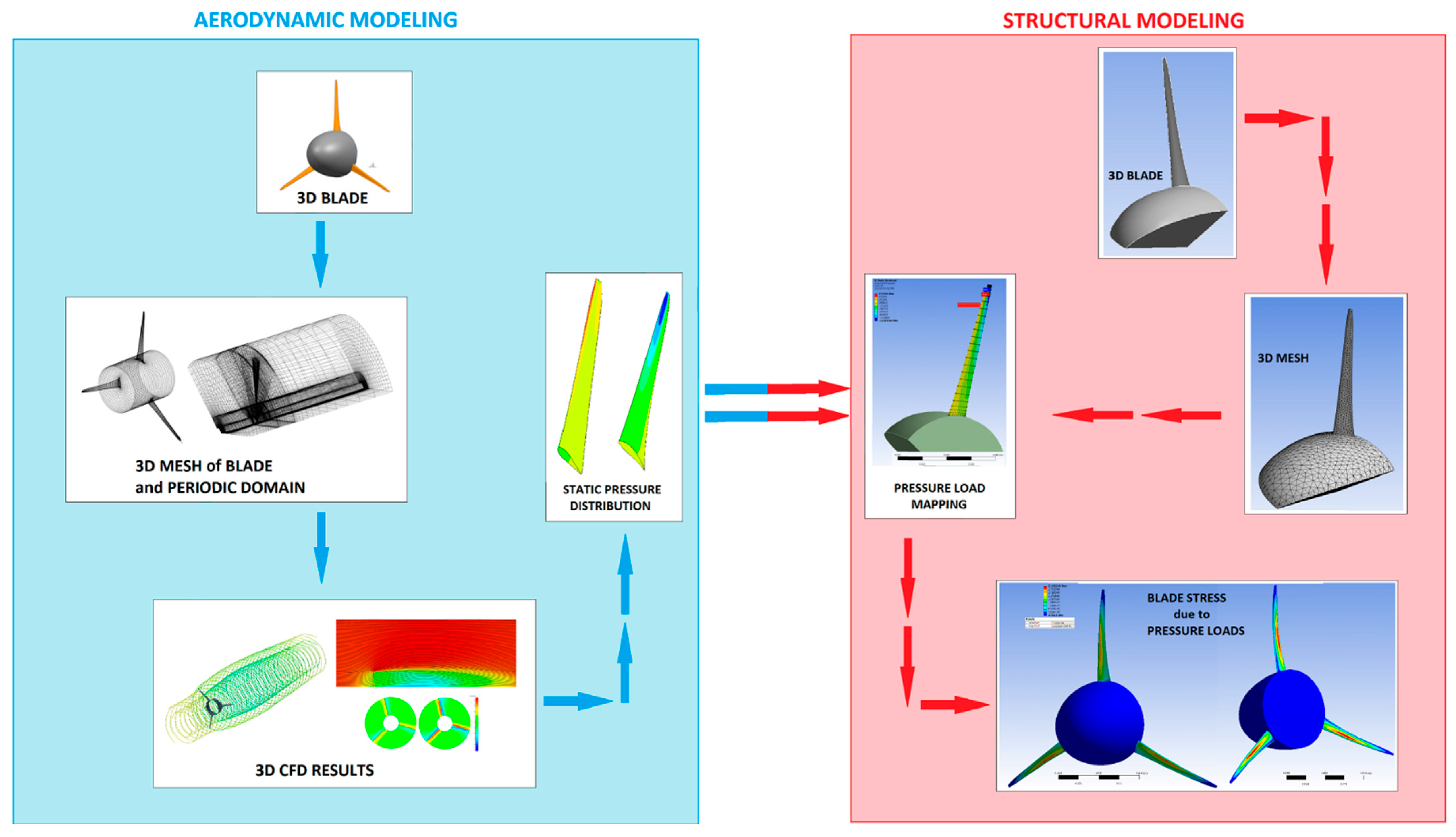
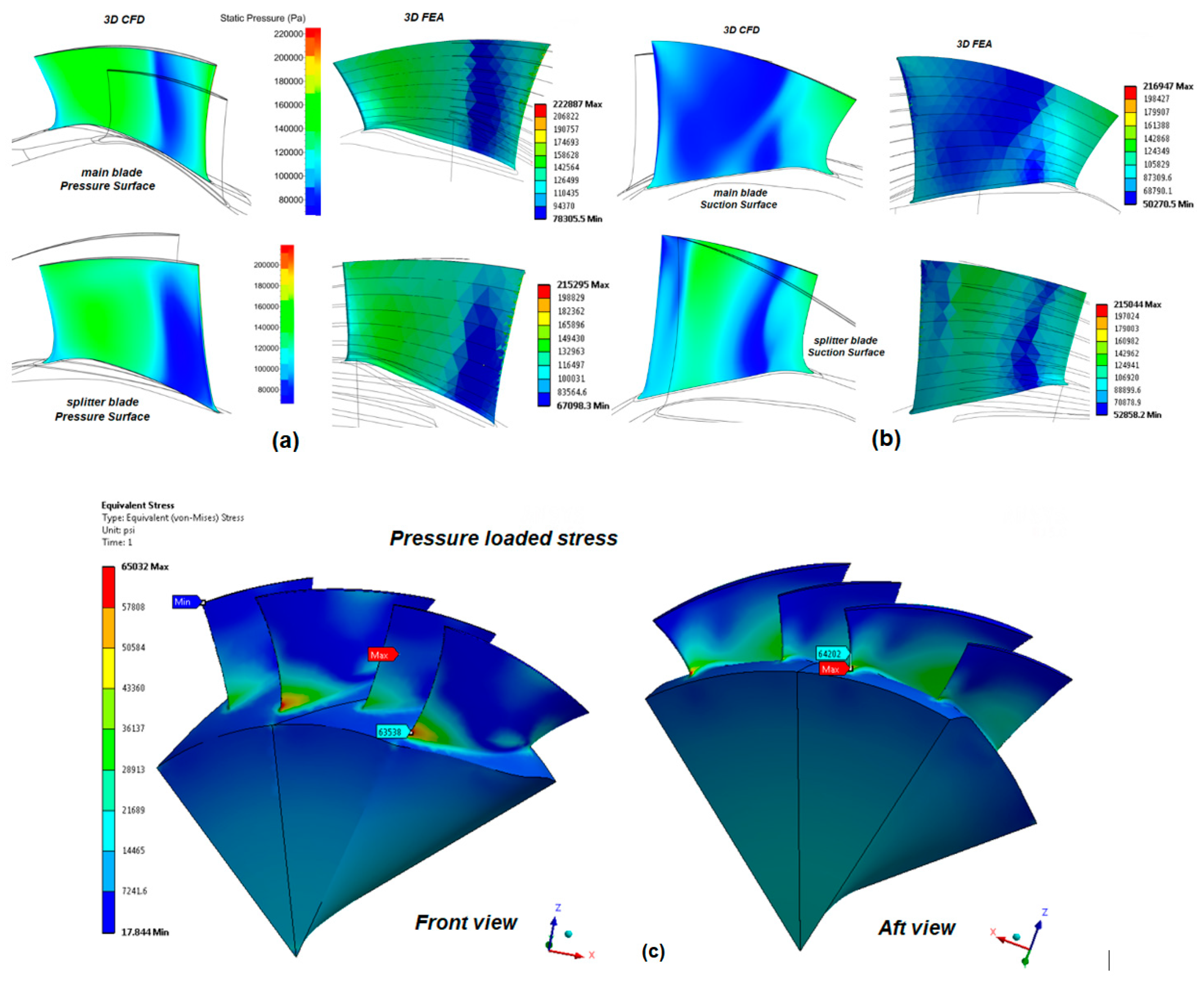
2.5.10. Fluid–Structure Interaction

Structural integrity of the rotor improves the lifecycle of the device and reduces maintenance and other costs associated with it. Aeroelastic behavior becomes important in unsteady flow fields and blade deflections. Mechanical stress, fatigue, and crack drastically reduce the system performance and need to be addressed in low- and high-fidelity multiphysics simulations. Blade geometry CAD is created by importing 3D airfoil sections and lofting them in a CAD package. ANSYS Mechanical is used for a centrifugal load-based analysis in 3D with appropriate constraints and boundary conditions. As the aspect ratio changes and the fluid becomes denser, deflections due to pressure loads rather than centrifugal loads become dominant and must be analyzed. Figure 10 shows the process of 3D stress analysis for any rotor using the pressure load from a 3D CFD solution.

3. Results

Several numerical simulations of ducted and unducted turbomachinery using the developed and existing multifidelity multidisciplinary design, analysis, and optimization tool chains are demonstrated. Bridging the gap between low- and high-fidelity domains enabled the utilization of several advanced concepts, such as smooth parametric geometry manipulation using B-splines, and complex compressible and incompressible flow physics including vorticity and vortex dynamics.

3.1. Ducted Axial Turbomachines

The MDAO framework is applied to several ducted axial turbomachines, as discussed in this section. Parametric geometry manipulation at low- and high-fidelity levels coupled with physics solvers and an optimizer creates optimum designs which are not always intuitive.

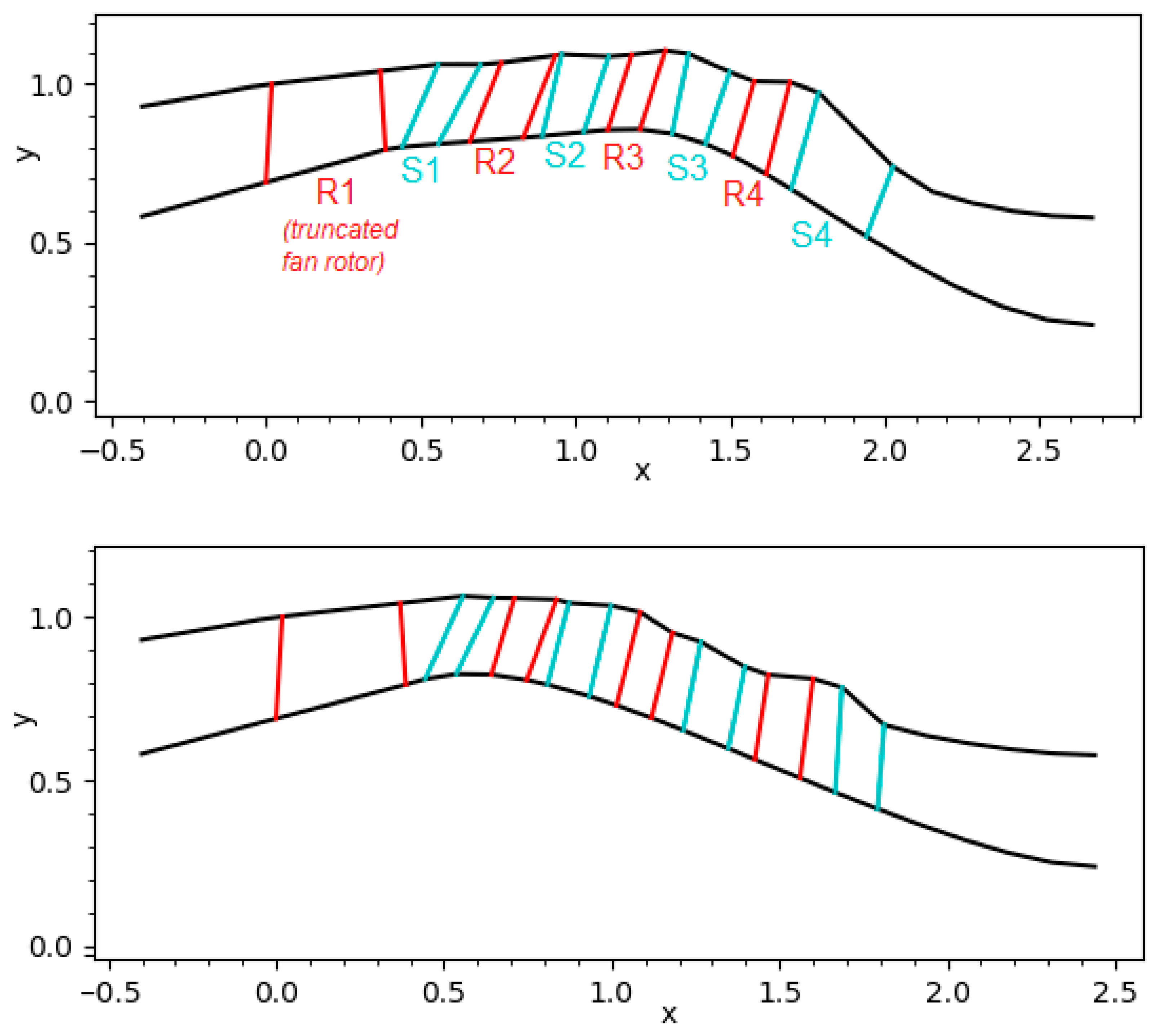
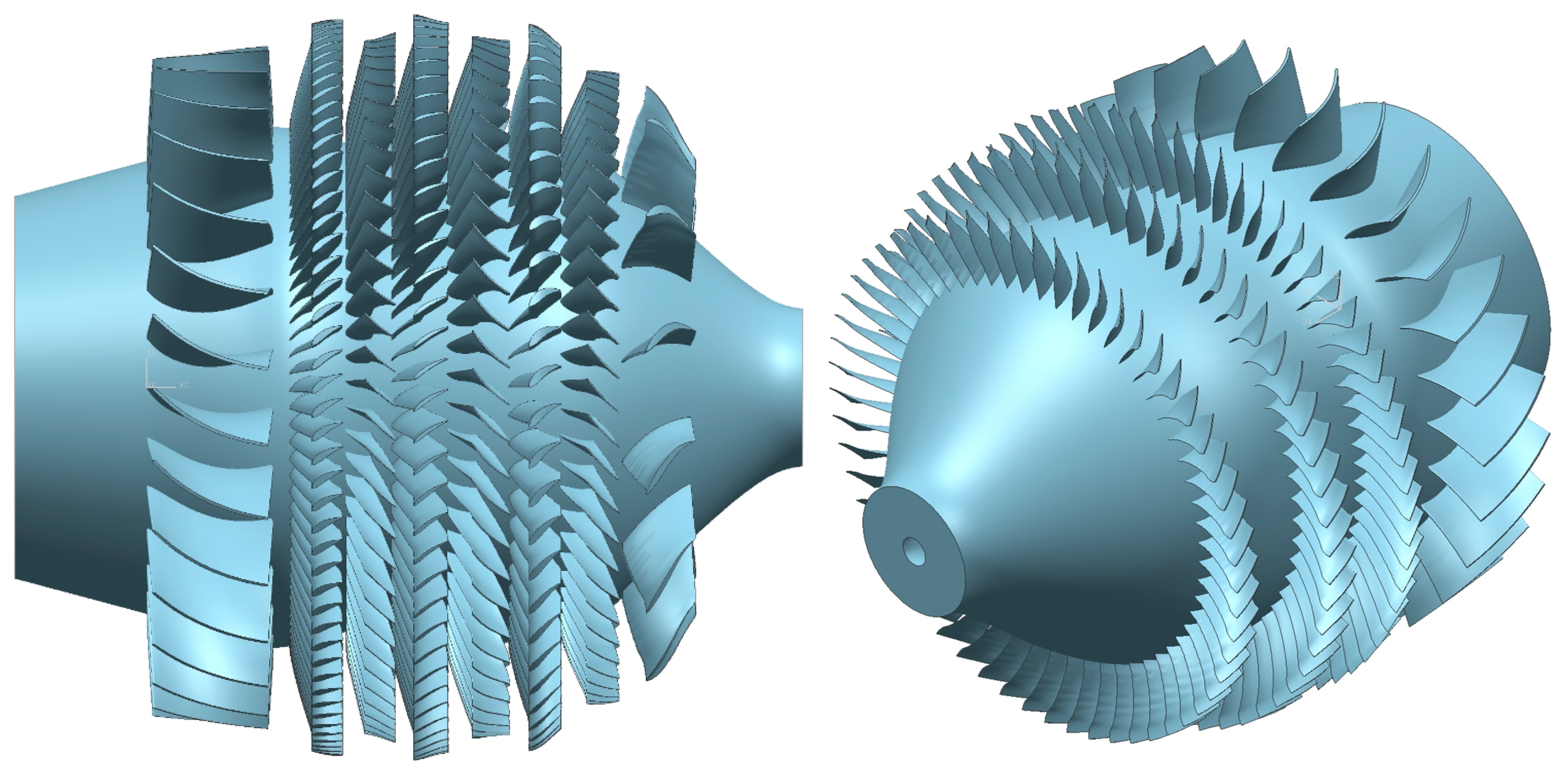
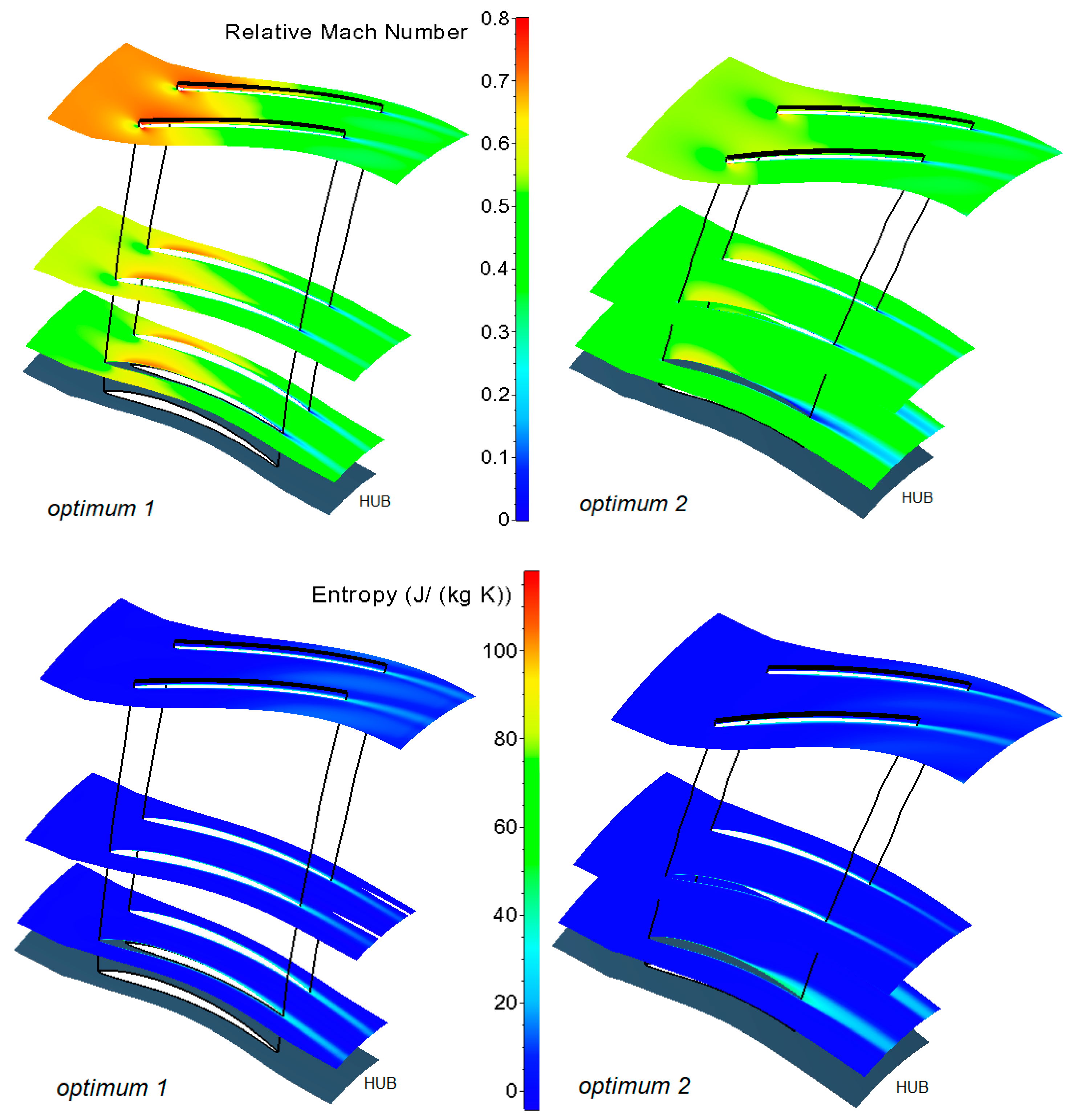
3.1.1. Multistage LPC Rotor with Optimized Flow Path

Rotor 3 of a fan stage and three-stage LPC configuration, as shown in Figure 11, is analyzed in 3D CFD and modal analysis is performed as part of the mechanical stress analysis. It spins at a low RPM of 3538, has 4 stages with high curvature, and has an overall total temperature rise of 90.61 K. T-Axi with coupled boundary layer and loss models defines the flow path, blade count, free vortex-driven blade designs with flow angles, chord, taper ratio, and length, among others. Park et al. [66] connected DAKOTA with T-Axi and optimized the LPC configuration for several objective functions using MOGA. The fan rotor, R1, was truncated to have the same mass flow as the LPC and was kept fixed in the optimization to maintain constant work by the fan rotor. The remaining amount of work was varied among the three rotors of LPC. In the optimization, 53 design variables were varied, including Mach entering each rotor (3 parameters), velocity ratio across each rotor (3), work split (3), stator exit angular momentum (3), blade taper ratio (7), hub and tip axial gaps (14), blade count per row (7, discrete), and flow path hub spline control points (5 parameters, 3 x, r coordinates, with 1 colinear). The multi-objective function was to maximize adiabatic efficiency, η, LPC mass, length, rotor and stator blade counts. Constraints imposed were the strength of the material for the ring disk and no separation in the boundary layer. Park et al. [66] carried out 25,000 function evaluations with titanium material properties to obtain a pareto distribution for mass and adiabatic efficiency. Two optimums with the resultant flow path, as shown in Figure 11, were chosen to analyze in higher fidelity, of which optimum 1 had a low mass (88.5%, 280.3 kg) and optimum 2 had a high efficiency (90.1%, 346.8 kg). These optimums were further initialized in a gradient-based optimization to increase the efficiency by varying the work split among the three rotors, as explained in detail by Park et al. [66].

Outputs from T-Axi optimums are used to generate 3D blade shapes and the CAD is as shown in Figure 12. The hub and casings are of high curvature for rotor 3, and for the isolated rotor 3D CFD, first and last displaced streamlines are used as hub and casings due to the thick boundary layer developed [66]. The generated 3D blade shapes are not optimized but they are defined by axisymmetric optimums. Inlet boundary conditions are an absolute total pressure of 209.752 kPa, total temperature of 363.93 K, spanwise definition of flow angle, β, from T-Axi, and streamline slope, φ. Outlet boundary conditions are static pressure imposed using radial equilibrium at 198 kPa, and the blade is spinning at 3538 RPM. The 3D CFD adiabatic efficiency for rotor 3 of optimum 1 is 91.25%, as compared to 93.47% from the T-axi axisymmetric optimum. Similarly, the 3D CFD adiabatic efficiency for rotor 3 of optimum 2 is 93.17%, as compared to 95.27% from the T-axi axisymmetric optimum. Figure 13 compares both optimum designs using relative Mach and entropy contours at several spanwise cuts. There is a corner separation in optimum 2, as seen in the cut plane near the hub. High-fidelity analysis demonstrates lower performance due to 3D effects as compared with low-fidelity optimums and can be further optimized using a parametric blade creator and 3D CFD solver connected to DAKOTA. Mechanical analysis is also a part of the framework described and is essential to manufacture/3D-print these devices for experimental testing. Figure 14 shows a tetrahedral mesh with 94,623 elements for rotor 3 as part of the structural analysis and all 14 modes of the nodal solution. New sets of optimization runs were performed with a very large number of function evaluations (100,000) for the titanium case, and Figure 15 shows the paretos for η vs. mass, η vs. length, and length vs. LPC mass. It is important to rule out any factors which might mislead the designer from obtaining a true optimum. Paretos obtained were slightly different than those obtained in the optimization with 25,000 function evaluations by Kevin et al. [66].

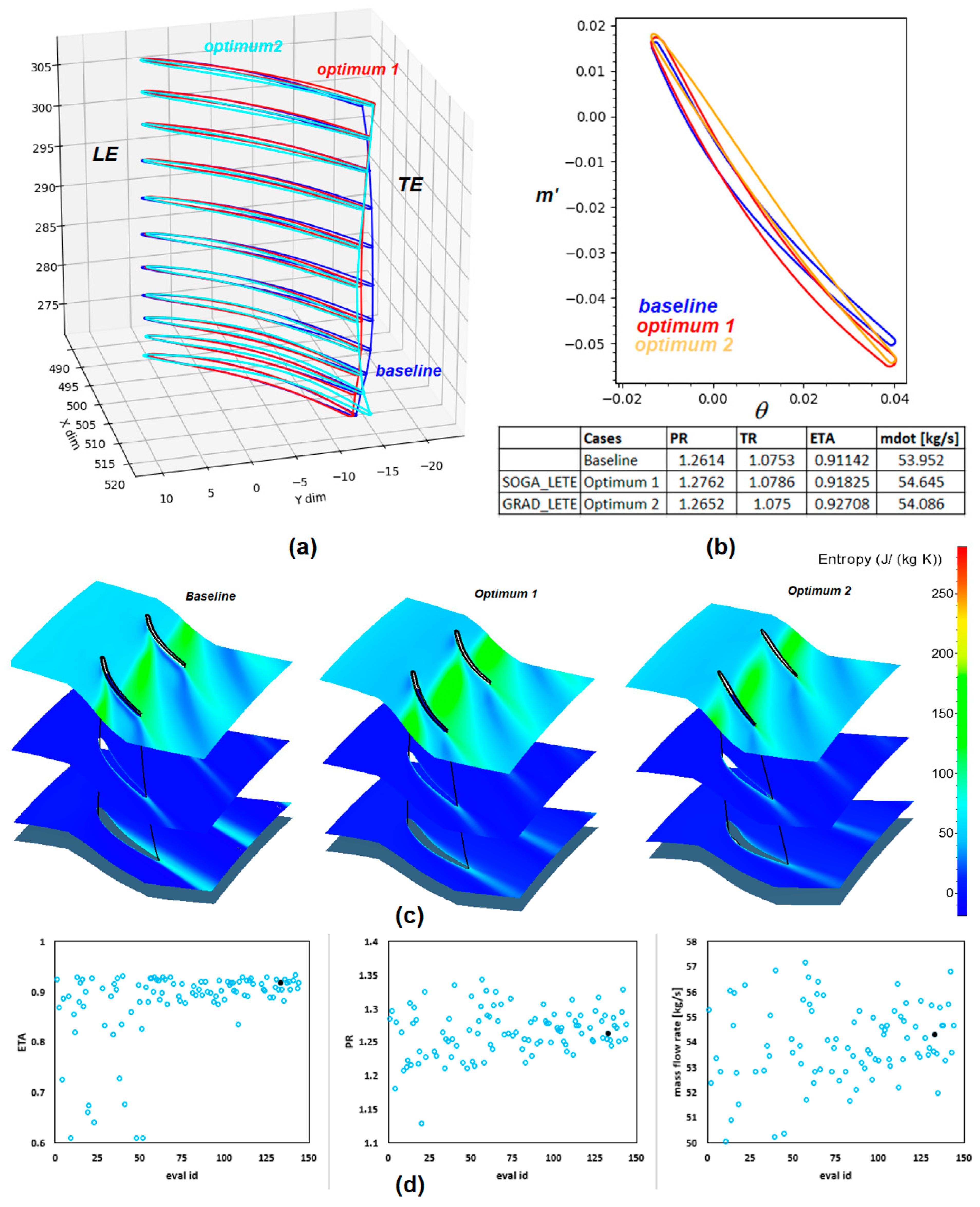
3.1.2. E³ HPC Rotor 6 Optimization

SOGA-based 2D optimization of several spanwise airfoils for rotor 6, representative of E³ HPC, is demonstrated using the curvature-driven meanline definition and MISES quasi-3D simulation. Three chordwise definitions of meanline curvature using B-spline control points, incidence, deviation, and LE droop, are varied in the optimization to generate 2D airfoils. Inlet and outlet slopes are constrained, and the objective function is to minimize pressure loss in MISES runs. Input for MISES is created by running the axisymmetric solver T-Axi before the optimization. Figure 16 shows Cp for the baseline and optimum airfoil at 25% span with a minimized loss coefficient from MISES. The pressure loss, $\overline{\omega }$, is reduced from 0.07186 to 0.02464, as shown in the figure.

The 3D optimization of a representative E³ HPC rotor 6, as defined in a NASA report [67], as a baseline is also demonstrated using spanwise variation of chordwise meanline curvature and inlet–outlet blade angles. Mahmood et al. [68] added the capability of spanwise parameter variation using the B-spline routine developed by the first author for the geometry generator. The 3D RANS is used to evaluate isentropic efficiency with inlet boundary conditions derived from T-Axi. Normalized velocity components are used to define spanwise flow angles and total conditions for pressure and temperature, as described by Mahmood et al. [68]. Static pressure is defined at the outlet, with radial equilibrium definition at the hub. The objective function was to maximize the isentropic efficiency while constraining mass flow and the total pressure ratio. The 18 geometric parameters that are varied are 3 curvature control points (u, curv) chordwise for hub, midspan, and tip-span locations, and 3 control points for spanwise incidence and deviation perturbation. SOGA and GRAD methods of optimizations were carried out to obtain optimum 1 and optimum 2 designs, as shown in Figure 17. A maximum iteration of 100 and 2000 function evaluations with a population size of 18 was initiated for the SOGA run. These are heavy computations due to the 3D CFD cycle time involved in the process. The GRAD method used was ‘conmin_mfd’, with a maximum iteration of 300 and convergence tolerance of 1 × 10⁻⁶. Figure 17 shows blade shapes for baseline and two optimums, as well as tip airfoils in Figure 17a,b. Entropy is minimized using the spanwise blade angle definition and airfoil shape, as seen in Figure 17c. Spanwise cuts show the flow improvement. Figure 17d also shows the evolution of the optimization by plotting objective functions with each evaluation and showing the optimum, represented by black dots.

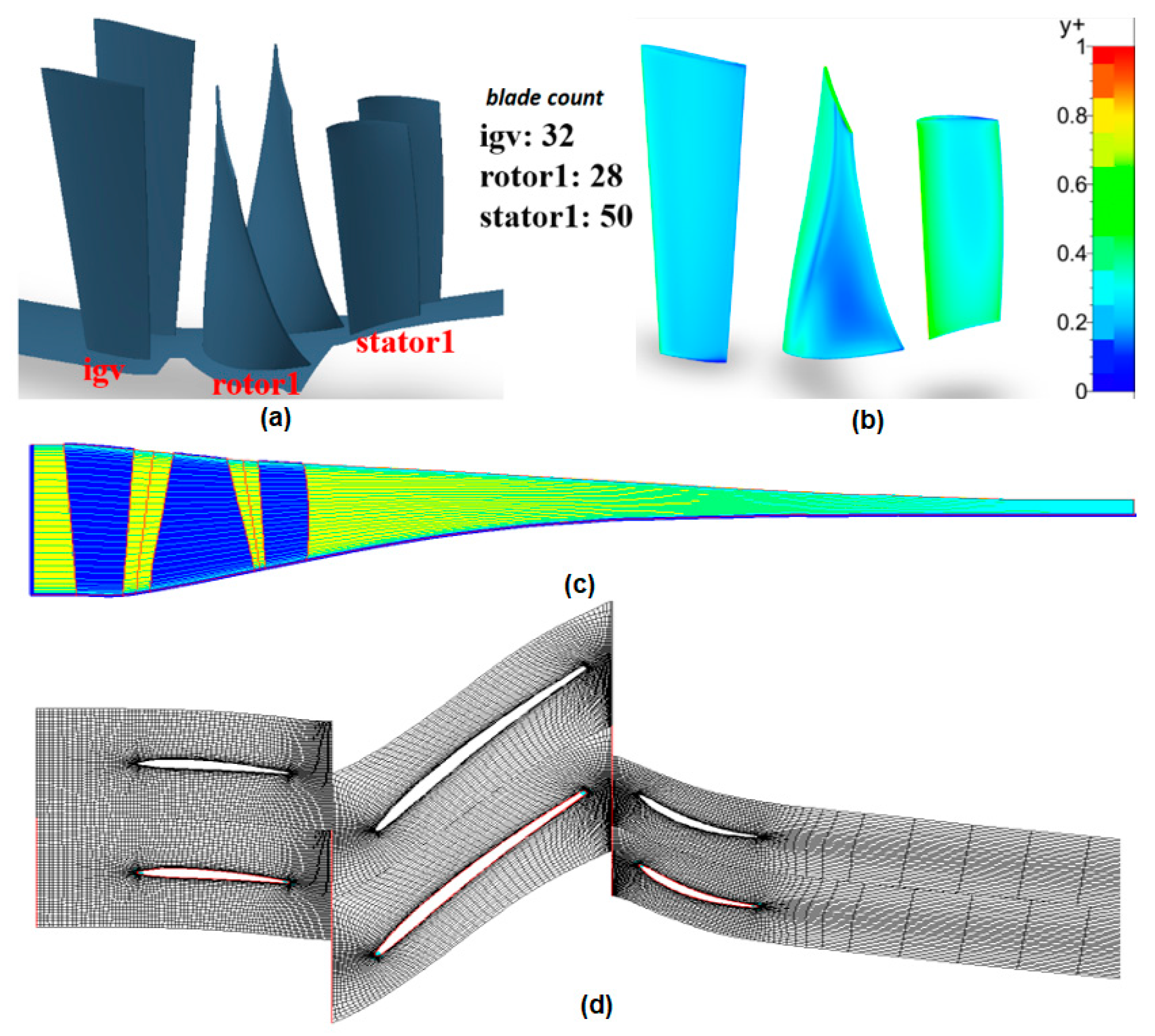
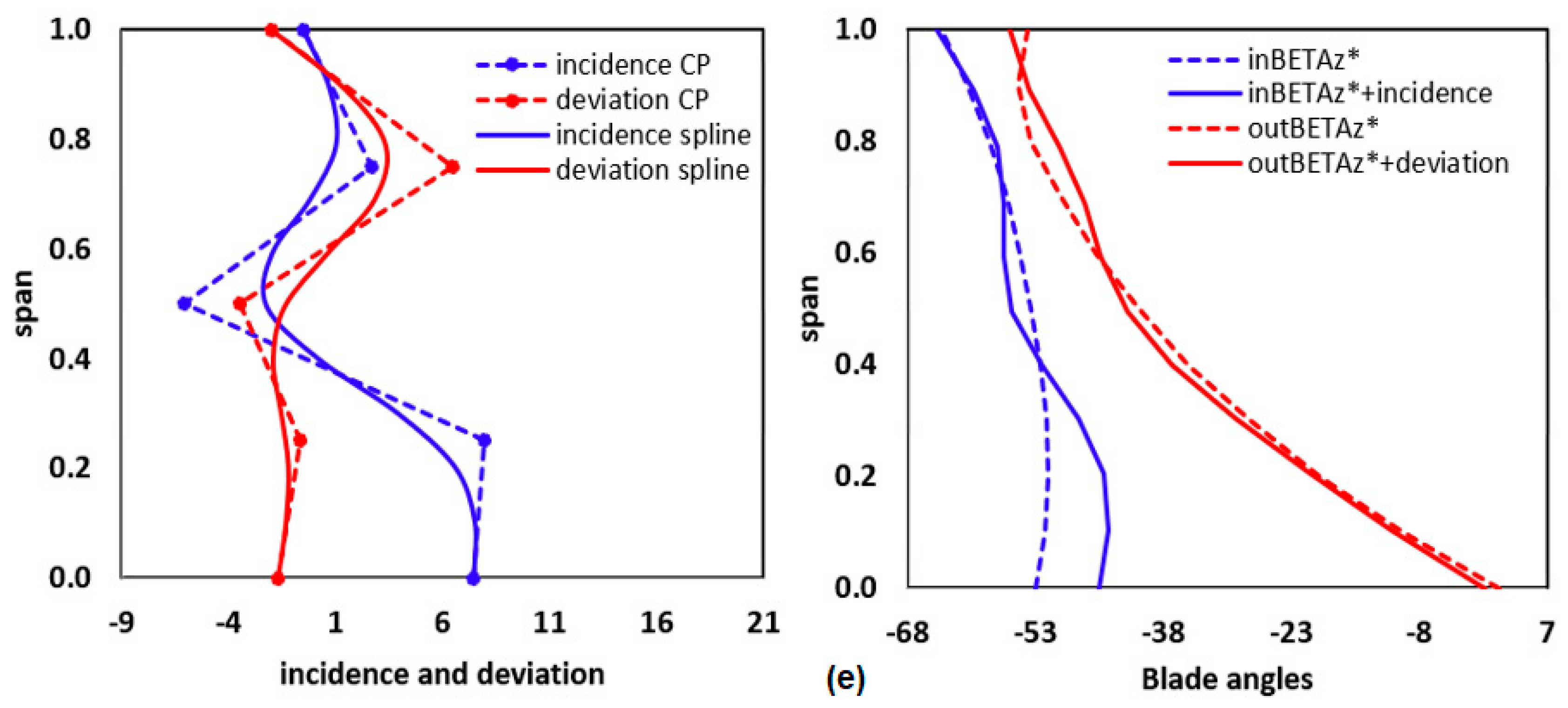
3.1.3. Optimized Rotor of 1.5 Stage E³ HPC

To illustrate the advantage of design optimization with spanwise geometry manipulation using splines defined by control points for a multistage design, the IGV and first stage of the E³ HPC representative configuration of the NASA–GE collaboration in the 1980s [67] is chosen as the baseline case. The rotor is optimized and analyzed in detail in a multi-stage, periodic, steady 3D CFD. Spallart–Allmaras turbulence model is implemented, and a steady mixing plane between each blade row with a mesh count of 1,550,000 with desired topology is used [68]. Total pressure and temperature with axial flow are imposed at the inlet. Static pressure ruled by radial equilibrium is imposed at the outlet. The chordwise control points defining the airfoil meanline curvature are connected through a smooth cubic B-spline in the spanwise direction and defined by additional spanwise control points [68]. The baseline design uses axial and radial coordinates at the leading edge, trailing edge, and the metal angles, as defined in the report [67]. Design specifications used for the optimization are detailed by Chen et al. [69]. The geometric parameters for optimization are the leading and trailing edge angles as well as the curvature of the meanline. These adjustments have been made sequentially: first, angle modifications, and then curvature modifications. The geometry for the 1.5-stage compressor and y+ on the blade surfaces is shown in Figure 18a–d. Phase 1 optimization was performed to obtain the best spanwise metal angle definition with default airfoil shapes for the rotor. Inlet and exit angles were given a spanwise perturbation as incidence and deviation, and the optimum values obtained are shown in Figure 18e. The genetic algorithm optimization framework using DAKOTA was implemented with a population size of 12 and 100 maximum iterations. The objective function was to optimize the adiabatic efficiency with 10 parameters of 5 control points at LE and TE, which define spanwise blade angle perturbation. CFD analysis was run in every iteration by replacing the rotor shape in the multistage setup, keeping the IGV and stator shape unchanged. This resulted in a 1.5% higher mass flow rate, with negligible change in efficiency.

The Phase 1 optimum rotor was further used in Phase 2 optimization as a baseline by varying the meanline curvature of the airfoil chordwise and spanwise using cubic B-spline control points. At each span, six chordwise control points (u, curv) define the curvature, of which the first and last two have zero curvature to clamp the spline at LE and TE. This definition is smoothly repeated for all five spanwise locations to create a 3D blade. In this optimization, there were three control points for curvature definition (curv) at fixed chordwise locations and one chordwise location itself (u) varied, and this was defined at five spanwise locations where the hub and 25% spanwise variables were identical to each other. Hence, 16 geometrical parameters (4 per span) were varied in total. In Figure 19, chordwise curvatures for all the spans are plotted, and for spans above 75%, there exist 2 inflection points where the curvature changes direction, which leads to an S-shaped airfoil. This optimized 3D shape has a better pressure gradient compared to the optimum of Phase 1, as shown in Figure 19, which also indicates flow separation minimization due to the improved radial flow. Hence, a stage efficiency of 88.08% is achieved with an improvement of 1.67%, and an isolated rotor efficiency of 90.66% is achieved with an improvement of 1.42%.

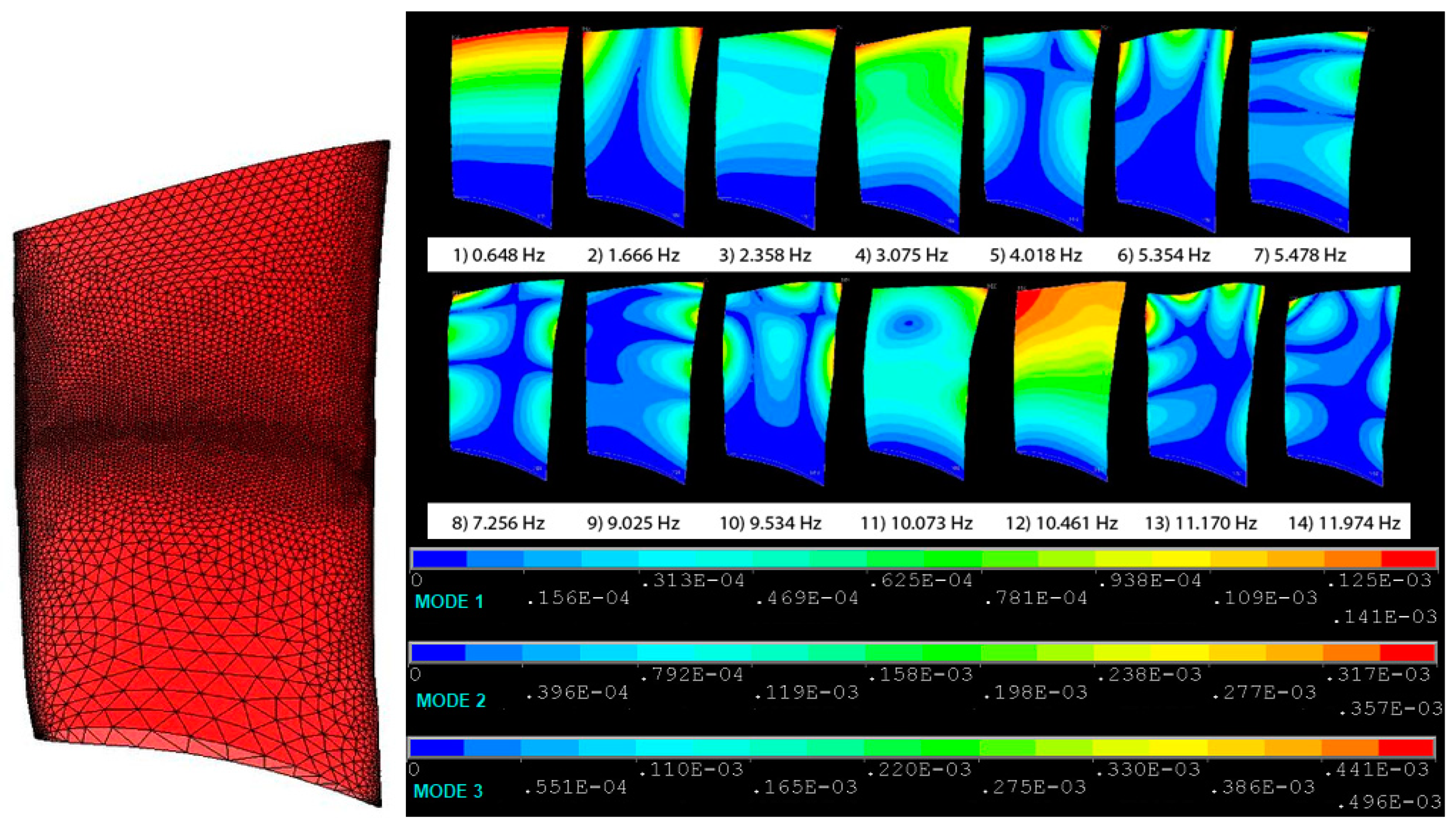
3.1.4. Fluid–Structure Interaction of Transonic Splittered Fan

A transonic splittered fan design is used to demonstrate the one-way fluid–structure interaction, where the pressure loads are imported from 3D CFD steady analysis into the FEA solver. Nemnem [37] designed and optimized the fan using the current framework with minimal radial stress and reduced mass, and using this optimum, further optimized the adiabatic efficiency. The authors, in collaboration with Somtrakool [70], developed a method to map steady static pressure load from a 3D CFD simulation on to 3D CAD of the transonic fan to analyze mechanical stresses under this load, as shown in Figure 20 using ANSYS Mechanical solver. A periodic sector of the fan is used for the stress analysis and the details of the creation of this sector are provided by Nemnem [37]. The aluminum alloy, 7075-T6, is used for the analysis, with a density of 2804 kg/m³, tensile yield strength of 503 MPa, ultimate tensile strength of 572 MPa, and modulus of elasticity of 71.7 GPa. The hub sector was constrained to analyze only the blade stresses. The fan operates at 27,000 RPM, which is 100% speed. Under pressure load, maximum stress was 448 MPa < 572 MPa (strength). Accuracy of the stress analysis depends on the accuracy of the captured physics in 3D RANS solution for transonic devices with shocks present in the flow passage.

3.1.5. Preliminary Design for a Distortion-Tolerant Turbofan Stage

Traditional airplane jet engines are installed below the wings, with clean flow at the inlet. Along with enormous thrust, a substantial amount of drag is also created due to the engine itself. A novel idea of improved propulsion is to place these engines at the tail of the aircraft with the boundary layer ingested flow at the inlet or distorted inlet. Essentially, the turbofan is designed to account for the boundary layer at the inlet, which brings low-momentum fluid into the nacelle [71,72]. The acceleration of this low-momentum fluid through the fan creates smaller wakes and less mixing loss downstream, which results in improved thrust and reduced drag. A non-axisymmetric outlet guide vane for the turbofan becomes necessary to address the distorted flow entering the rotor and exiting with a non-axisymmetric swirl, as described by Sandeep et al. [73]. Non-axisymmetric spanwise lean is used to minimize the entropy [74,75]. A preliminary design approach is needed to define a good baseline for high-fidelity optimization. Isentropic relations are used to size the device, assuming efficiency. The work performed is calculated and the inlet Mach number is iteratively obtained, as explained in Figure 3. The meanline design tool, TC-DES, was used to calculate blade properties, spanwise work distribution, and the flow path for the turbofan. Figure 4 shows the velocity triangles spanwise for the rotor. This is followed by an axisymmetric solution using T-Axi, which defines the blade row performance, including the diffusion factor, flow and stage coefficients, stage reactions, and pressure losses. T-Axi also calculates geometrical parameters such as solidity, stagger angles, LE and TE locations, and streamlines for 3D blade generation. An axisymmetric solution-based optimization is performed to obtain the best spanwise angular momentum distribution, lower rotor and stator solidity, better diffusion, and higher efficiency, as shown in Figure 21.

The goal was to load the tip region more than the hub region to minimize end-wall losses defined in T-Axi [73]. ‘Baseline 2′ in the figure is the chosen optimum for 3D analysis.

3.1.6. Axial Turbine Design for a Small JetCat Engine

The JetCat turbojet engine is a type of micro-jet engine designed and manufactured by JetCAT [76]. As part of an outreach program between the University of Cincinnati, Cincinnati, Ohio, USA and the Air Force Research Laboratory, US Air Force Base, Dayton, Ohio, USA, the objective was to design an exhaust-driven fan with a 12-inch diameter for a JetCat P80-SE engine, which has a 4.4-inch diameter, weighs 2.9 pounds, and produces a thrust of 22 pounds at an RPM of 125,000. An ungeared propeller connected to an exhaust turbine with a transition duct was chosen to be designed and analyzed using the current MDAO framework. It was planned to be manufactured and attached to the JetCAT aft of the nozzle. Senior year aerospace engineering students collaborated with the authors and Ahmed Nemnem [37] to create the designs, starting from a low-fidelity tool, moving up all the way to high-fidelity 3D CFD analysis. A preliminary turbine stage was designed using T-Axi along with the transition duct, and the spanwise airfoils were analyzed in MISES, as shown in Figure 22a, to eliminate flow separation through varying thickness, meanline curvature, and metal angles. Blade counts for the turbine stage were calculated iteratively using Zweifel numbers to eliminate separation and frequency effects from the three struts in the transition duct. A total of 27 vanes and 59 rotors were finalized. All these parts were decided to be manufactured using metal laser sintering by a company called SolidConcepts [77], assembled and tested at AFRL. Hence, several iterations of the blade designs with leading and trailing edge thickness for 3D printing and blade smoothness using the curvature-driven meanline option were analyzed. The power from this turbine stage was to be matched with an ungeared propeller attached to it at a chosen RPM of 20,500 and was also designed using the current framework [65]. Figure 22b,c also show entropy for the turbine stage, 3D CAD, and the additively manufactured product.

3.2. Ducted Radial Turbomachines

3.2.1. Single-Stage and Novel Centrifugal Compressor

A representative design of a NASA low-speed centrifugal compressor [78,79,80] is designed with a vaneless diffuser and optimized. The compressor has an inlet tip radius of 42.939 cm, exit radius of 76.22 cm, inlet Mrel of 0.31, RPM of 1862, 20 blades, back-sweep angle of 55 degrees, PR of 1.166, and a mass flow rate of 30 kg/s. Streamline coordinates, LE and TE shape, are obtained from the NASA report. Muppana and Mishra [56,57] created a 1D model to generate blade angles using a temperature ratio of 1.03 calculated from isentropic relations in collaboration with the authors. Euler-turbomachinery equations provide velocity components and an iterative inlet density calculation using the state equation output metal angles [57]. Using the geometry generator, a baseline design is created to optimize the rotor efficiency by using the metal angles from the 1D, airfoil camber-line with default thickness. Spalart–Allmaras turbulence model is used, with total pressure and temperature defined at the inlet and constant mass flow imposed at the outlet as boundary conditions. Different losses embedded in the 1D tool and obtained from a 3D RANS solution for the single stage are compared, as shown in Figure 23, in collaboration with Muppana [56]. The compressor is a representative design of Krain et al. [78] with a PR of 4, with 1862 RPM, mass flow rate of 4 kg/s, and 24 blades. Loss models in the low-fidelity tool are comparable to the high-fidelity solver, which is essential to capture better geometry at this level before 3D geometry can be created.

Spanwise variation of the chordwise airfoil camber-line defined by curvature is optimized. Three chordwise control points (u, curv) defining the curvature as a cubic B-spline are varied for three spanwise airfoils at the hub, midspan, and tip, with a total of eighteen parameters. Constraints applied on mass flow rate and pressure were to be within 0.5% of the baseline design. DAKOTA drove the entire cycle of geometry generation, 3D-mesh, 3D CFD, post-process, and output parsing for the defined objective function. The SOGA method was used with a population size of 12,100 function evaluations based on CFD. Optimization resulted in an S-shaped midspan and tip airfoil with 80% efficiency. The single-stage optimized configuration was further modified to create a novel centrifugal compressor. A novel dual rotor in collaboration with Abdallah [81] on the same hub and casing with vane in between them was created keeping the same amount of work done as in the single stage for comparison. Rotor 1 is designed as an axial rotor, a vane with a turning angle of 20 degrees, and second rotor as a purely radial rotor. The work split between rotors 1 and 2 is chosen to be 40% and 60%, since most of the work is performed by the second rotor. The pressure ratio for rotor 1 is 1.035, and for rotor 2 it is 1.14, which resulted in a total efficiency of 86% for the novel configuration calculated by the 1D model [57]. The blade count was kept constant at R1 = 20, S1 = 30, and R2 = 40. Optimization resulted in an improvement of 8.55% in efficiency, going from 80.41% (single stage) to 87.29% (novel) for the same mass flow rate and temperature ratio. The pressure ratio increased from 1.11 (single stage) to 1.143 (novel). Muppana [56] explored different work splits between the two rotors on the same disk as a function of the pressure ratio and efficiency and designed a higher-pressure ratio (PR = 4) version of the device. The ratio favored more work for the second rotor than the first. The real benefit in this design is that the addition of vane between rotors extends the design space, and flow can be turned more efficiently. Figure 24 shows the axisymmetric view of the absolute Mach number and Figure 25 shows total pressure compared at 95% span and entropy comparison between the single stage and the multi-rotor stage is shown at 50% span. Flow turning due to the stator reduces the relative velocity and converts the kinetic energy into static enthalpy at its inlet. Lower flow velocity reduces entropy moving further downstream. Future work would be to optimize the blade count and blade passage throats.

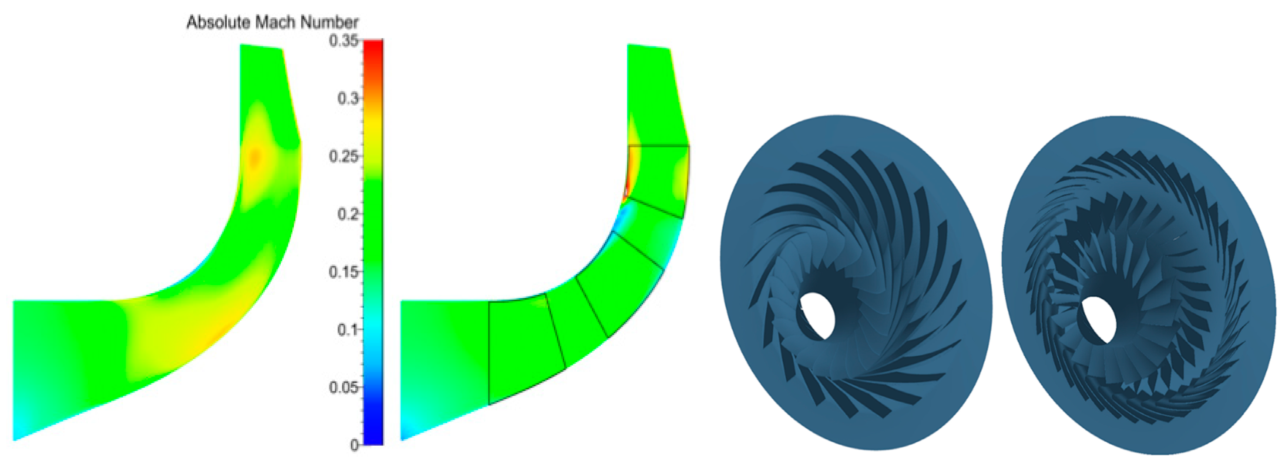
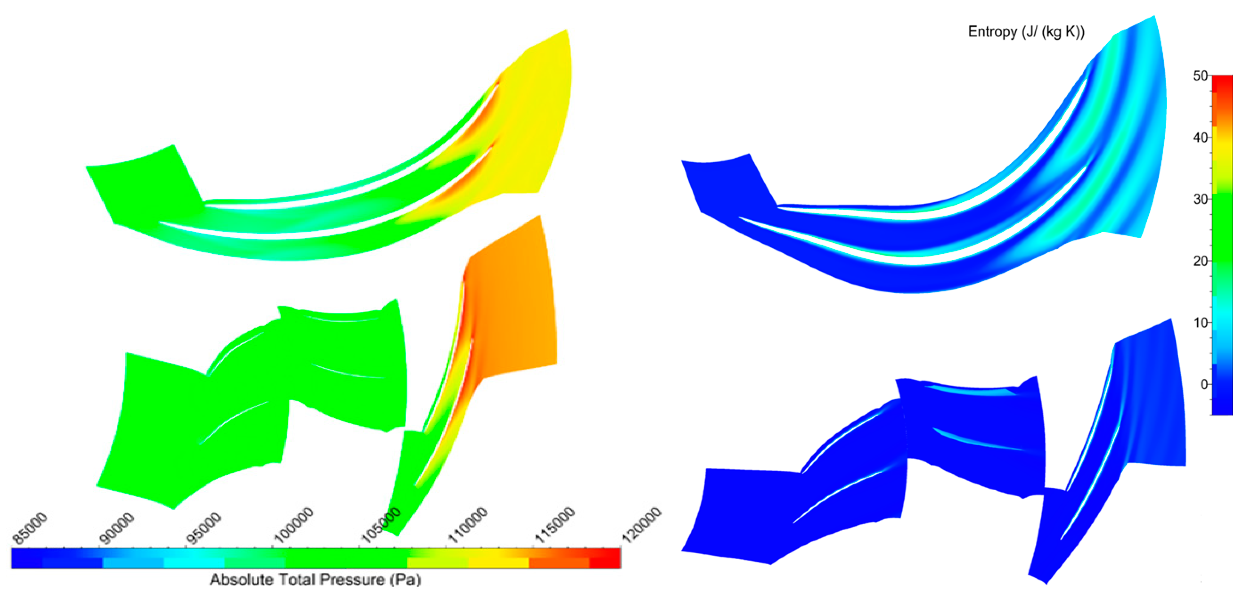
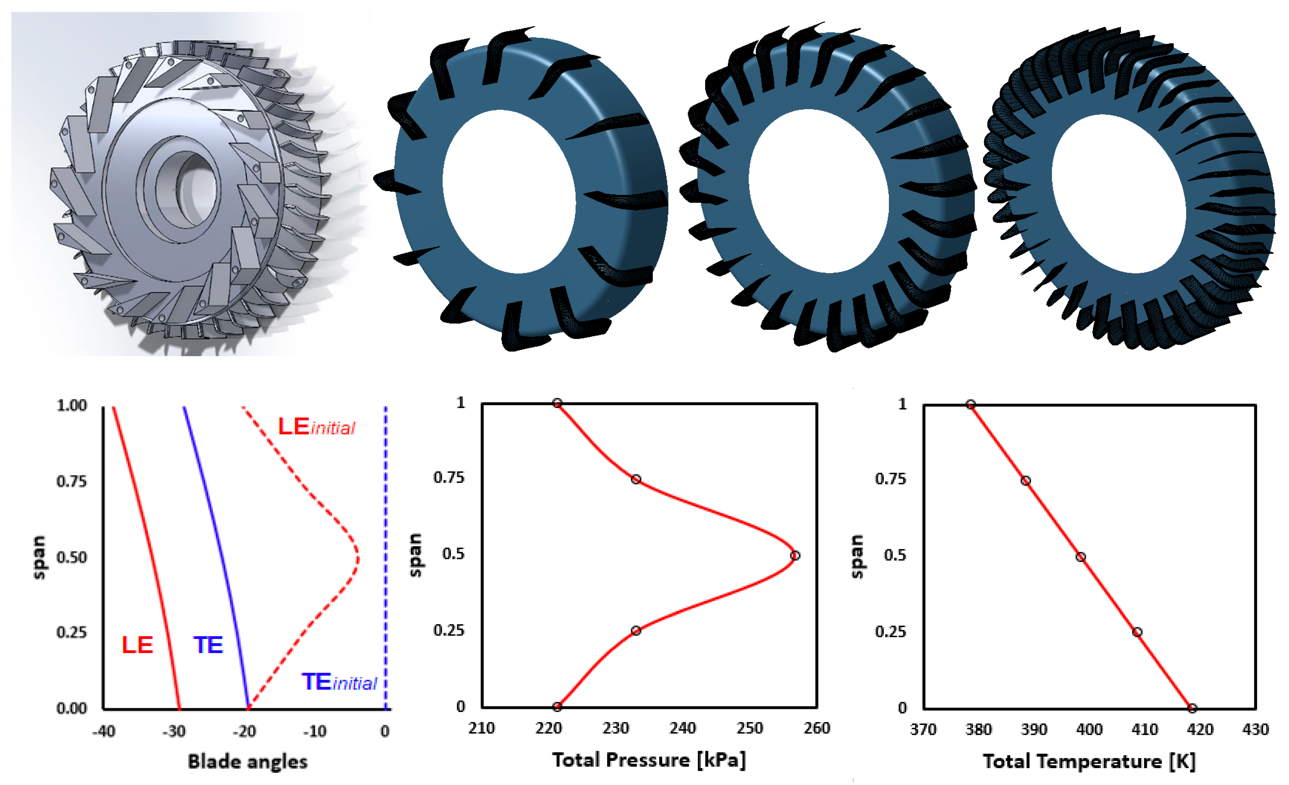
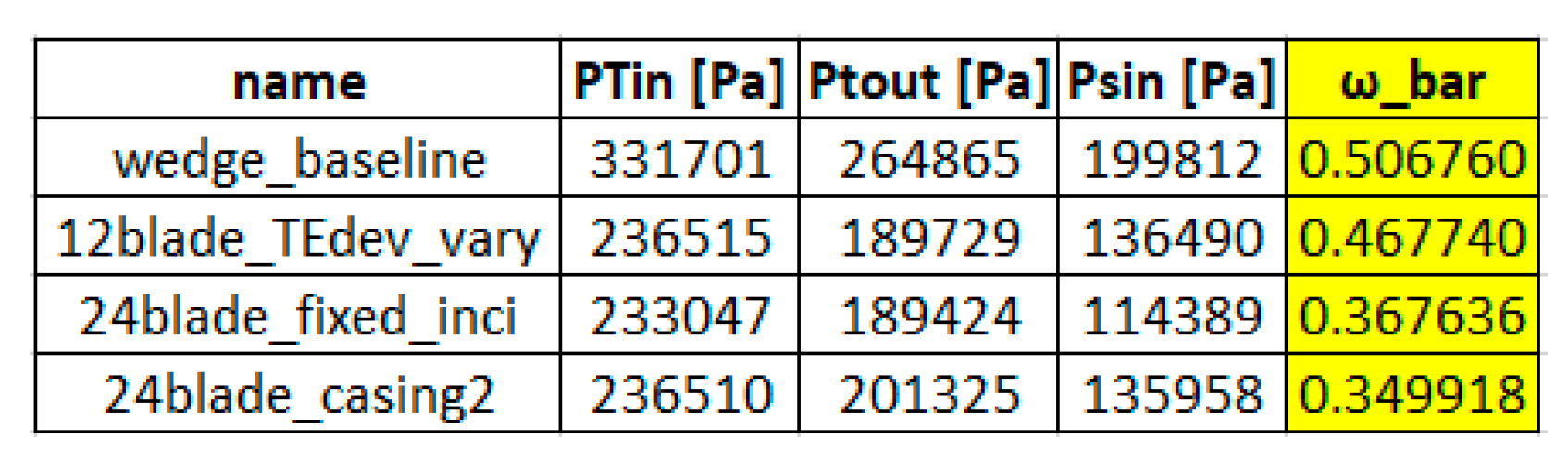
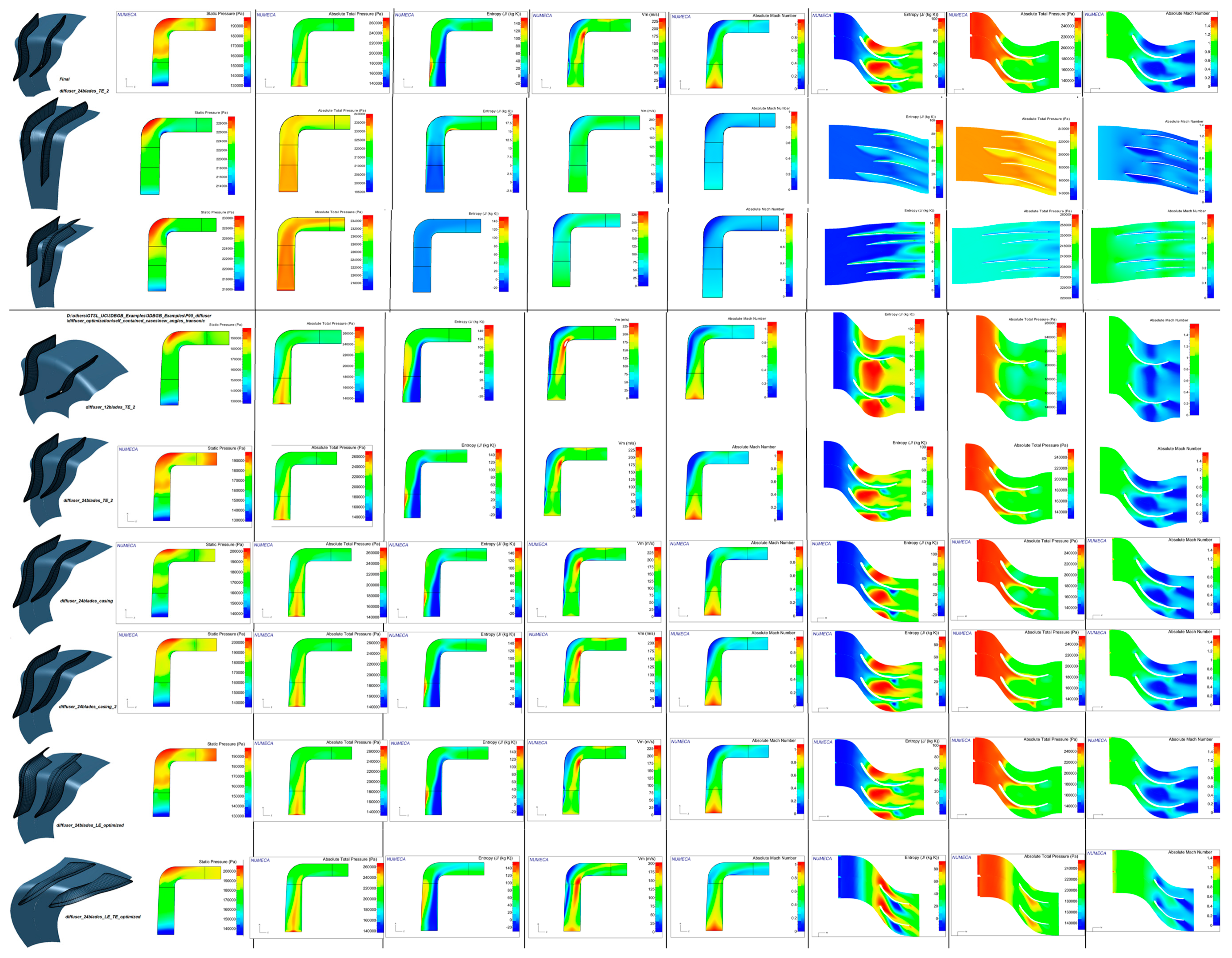
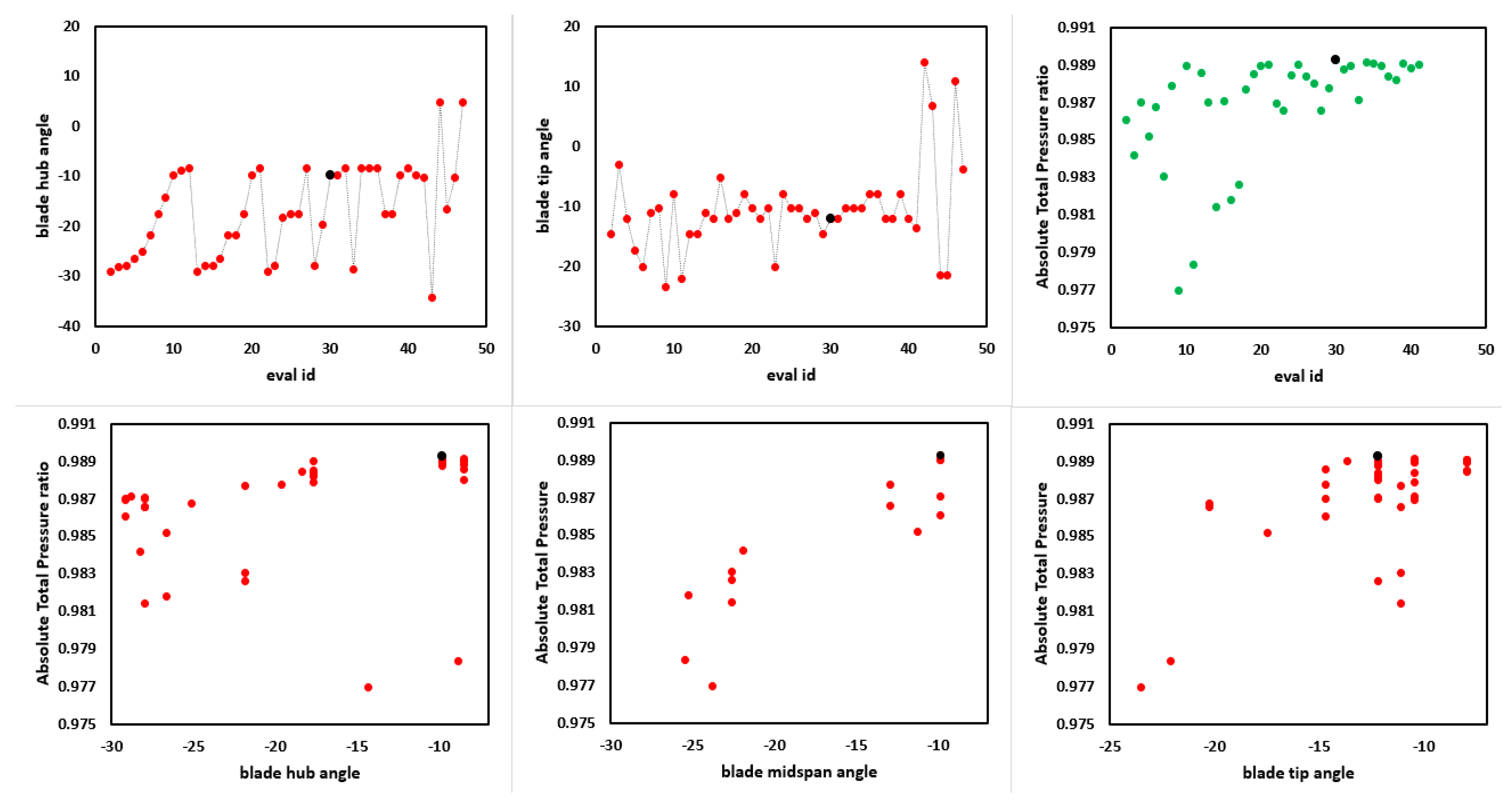
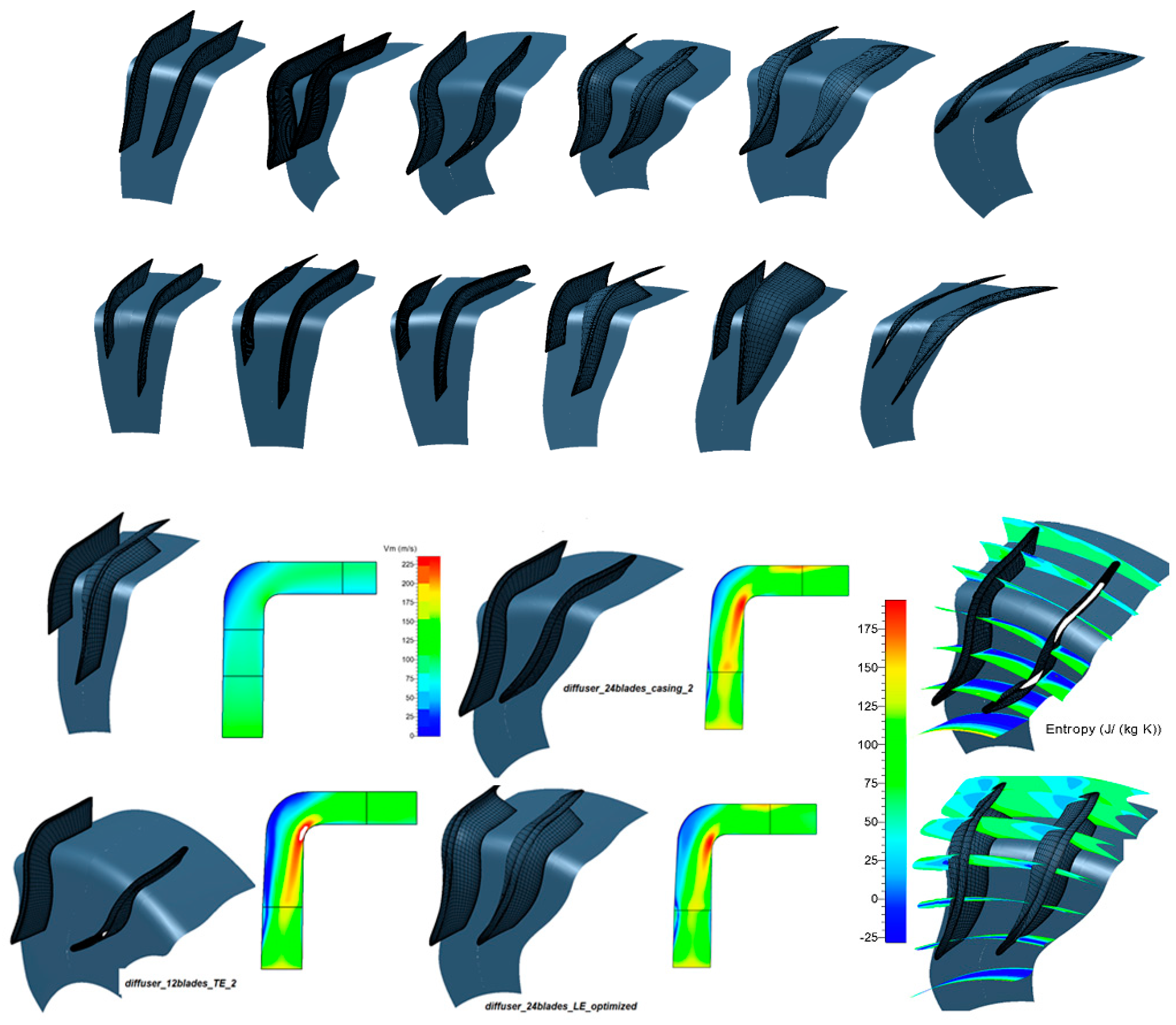
3.2.2. Radial Diffuser Vane for a Small Jet Engine

Demonstration of a radial diffuser redesign and optimization downstream of a centrifugal compressor for a small jet engine to improve performance is described here. JetCat P90 has a centrifugal compressor at the inlet followed by a radial diffuser and is connected to a combustor and an axial turbine. It produces a thrust of 23.6 pounds [76], with the radial impeller spinning at 125,000 RPM at rated power and a device diameter including the impeller and diffuser of 112 mm, with a mass flow rate of 0.24 kg/s. As part of the advanced propulsion challenge organized by the Air Force Research Laboratory, Dayton, Ohio, USA, the team at University of Cincinnati, Cincinnati, Ohio, USA chose to minimize diffuser pressure loss, working with the authors utilizing the current MDAO cycle. The existing diffuser has a two-stage radial wedge, a 90-degree bend passage, and a cambered axial vane, as shown in Figure 26.

A good baseline is always necessary to initiate the optimization process. A single blade vane with 24 blades was chosen instead of the wedge and cambered axial vane as part of the redesign. This would eliminate some performance losses at the blunt trailing edge of the wedge and the 90-degree turn. Obtaining the right metal angles for the radial diffuser was crucial and would also become a starting point to open the blade design space. A 1D momentum and energy conservation analysis using MATLAB was developed by Holden et al. [82] in collaboration with the authors for calculating the flow exit angle from the radial impeller at the operating point. Diffuser vane LE angles were set to these conditions, and TE angles were set to zero initially to minimize the exit swirl. A quick 3D RANS analysis showed that the TE angles must be redefined to minimize the swirl, as shown in Figure 26. Inlet boundary conditions for this analysis are a total pressure and temperature profile analogous to what the impeller exit generates, tangential and radial velocity ratios with default turbulent viscosity using Spalart–Allmaras turbulence, and extended wall functions activated. TE location was also moved upstream since the flow is purely axial after the 90-degree bend. Figure 27 shows the angles varied in each evaluation, the absolute total pressure for each iteration of the optimization parameter, and the optimum value, highlighted as black dots. Full-bladed and splittered versions of the redesigned radial diffuser were optimized. Several geometry parameters were varied in phases, including three spanwise LE and TE angles, and TE positions for full-bladed and splittered diffusers. Holden et al. [82] describes the entire process for the full-bladed diffuser and demonstrates the utility of this MDAO framework. TE thickness was also optimized in their work for enabling additive manufacturing of the diffuser and assembled with the impeller.

The splittered version of the diffuser is demonstrated here. Figure 28 compares the pressure loss calculated for the wedge baseline [83] and several optimums generated. Figure 29 shows various geometries created by DAKOTA to minimize the total pressure loss coefficient, which include some extreme cases. First, the LE angles were optimized, keeping TE angles as zero, then using the optimal LE angles, TE angles were optimized to obtain the best lean definition of the splitter. End-wall contouring was also useful in minimizing the losses, as explained by Holden et al. [82]. When manufacturing is considered, some of these optimums are not viable and the constraints need to be changed [82]. Figure 29 shows the meridional velocity of full-bladed and splittered diffusers in axisymmetric view and cross-stream cuts of entropy for some of the optimums. Automation of the entire process, including post-processing flow properties in axisymmetric and blade-to-blade views is achieved. It enables the designer to examine the flow physics generated due to parametric geometrical variation and choose a suitable optimum, as shown in Appendix A, Figure A1.

3.3. Unducted Rotors

A low-fidelity parametric design analysis tool, py_BEM, based on blade element momentum theory is developed to define spanwise chord, stagger, and airfoil types for high aspect ratio unducted rotors, such as propellers, helicopter rotors, wind and hydrokinetic turbines [62]. It also creates high-fidelity geometry inputs to generate 3D blade shapes through the blade generator. Figure 8 shows the connection with the DAKOTA optimizer to generate optimum spanwise geometrical parameters used for 3D blade shape creation and high-fidelity multiphysics analysis.

3.3.1. Contra-Rotating Propeller Rotor

Unducted propeller rotors are designed and optimized using py_BEM connected to DAKOTA with asynchronous parallelization, which reduces the optimization time by 2 orders of magnitude, from 100 to 1 min, with 40 cores (2 threads per core) of AMD Opteron 6344 [62]. A massive design exploration at the low-fidelity level can be performed to obtain several desirable configurations, such as optimal chord distribution, blade count, lift distribution using right airfoil, and blade twist for solo propellers. Contra-rotating propellers can also be designed and analyzed using py_BEM, which accounts for the exit swirl from the first rotor. Development of electric propulsion for urban mobility with several redundancies embedded must begin with a sizing study to explore the best rotor area, the power to thrust ratio, the rotor gap for torque balance, optimal thrust with equal and unequal splits between rotors, the blade count, and different tip radii for both rotors to take advantage of streamline double contraction [62]. Contra-rotating propellers are optimized for an urban mobility, four-armed octocopter to produce a thrust of 150 lbf per arm, with a vertical speed of 15 m/s and a hub diameter of 10 cm. SOGA-based optimization is performed, varying a total of 16 parameters, including the rotor tip radii, tip speed ratio, the rotor 2 RPM, and five spanwise chord multipliers for each rotor to create smooth B-spline-based chord distribution of an existing definition and blade count for both. AoA for each rotor was fixed at −4 degrees using ClarkY airfoil polar. An initial population size of 200 with 4000 maximum function evaluations, 2 parents and 2 off-springs, with a crossover rate of 0.8 and 7 generations, are defined for the SOGA-based optimization run. Thrust constraints for both rotors were to be less than 100 lbf each. The rotor gap is fixed in this optimization to take advantage of the exit swirl from rotor 1. Figure 30 shows progression of the optimization process through plots of a few parameters varied in each evaluation and showing the down-selection of efficiency. Black dots represent the optimal parameter obtained for highest efficiency.

The two-rotor system efficiency increased from 60% to 74% and the resultant spanwise distribution of chord, Reynolds number, and stagger along with their respective 3D blade shapes are compared in Figure 31. The baseline design had 3 blades for each rotor, and the optimum is 3 for rotor 1 and 5 for rotor 2, with thrust split slightly favoring the first rotor. This is purely a low-fidelity-based optimization without mechanical constraints. Figure 31 shows a shorter rotor 2, with a wider chord distribution. The twists of rotor 1 and rotor 2 are optimized for the best utilization of the rotor 1 exit swirl by rotor 2. Figure 32 shows the efficiency calculated for all evaluations and the varied values of 10 chord multipliers, rotor radii, tip speed ratio, and second rotor RPM in each evaluation, with black dots representing the optimal values. The tip loss model defined in the low-fidelity tool dictates the smaller chord choice above 80% span.

3.3.2. Wind Turbine 2D Airfoil Optimization

Highly staggered airfoils with optimal lift to drag ratios are used spanwise for high aspect ratio wind turbines to maximize power capture at low incoming wind speeds [84]. An application of 2D airfoil optimization driven by MOGA-DAKOTA cycle connected with XFOIL is demonstrated to generate high L/D airfoils at a specified Reynolds number. XFOIL is a 2D panel solver using inviscid/viscous coupling for calculating lift and drag coefficients at specified AoA of airfoils. The transition location on top and bottom surfaces of the airfoil is also calculated using an e⁹-type amplification of the Tollmein-Schlichting wave [63]. Subramanian [85], in collaboration with the authors, added the curvature-driven meanline and smooth thickness capability for highly staggered airfoils in the geometry generator through smooth cubic and quartic B-splines defined by control points. The objective function was to minimize f(x) defined as the sum of the C_d/C_l ratio at C_l = 0.5, 0.65, 0.8, and 0.95, for a Reynolds number of 7 × 10⁵, and similarly for 9.5 × 10⁵. These eight ratios are weighted equally to create the multi-objective function. The 21 parameters varied are 9 meanline curvature control points at fixed chord locations, 11 thickness control points also at fixed chord locations, and the total camber of the airfoil. The population size is set to 200, with 450,000 function evaluations using the genetic algorithm. The baseline was S809 airfoil of an experimental NREL rotor [86] in the same REYN and C_l range. Figure 33 shows an example of a single iteration in the optimization cycle, showing curvature defined by spline control points, airfoil creation, and C_p distribution for that airfoil obtained from the XFOIL run.

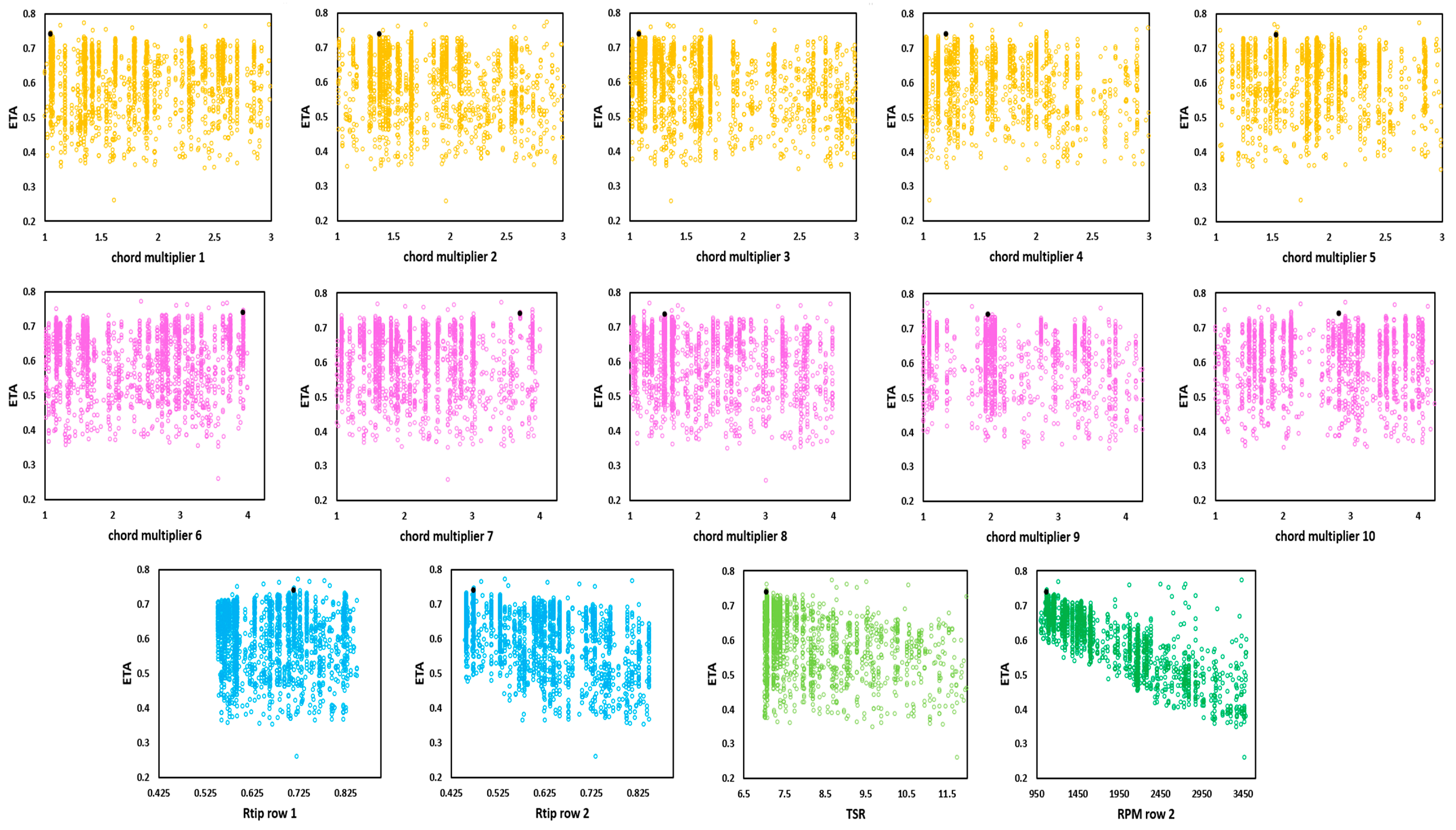
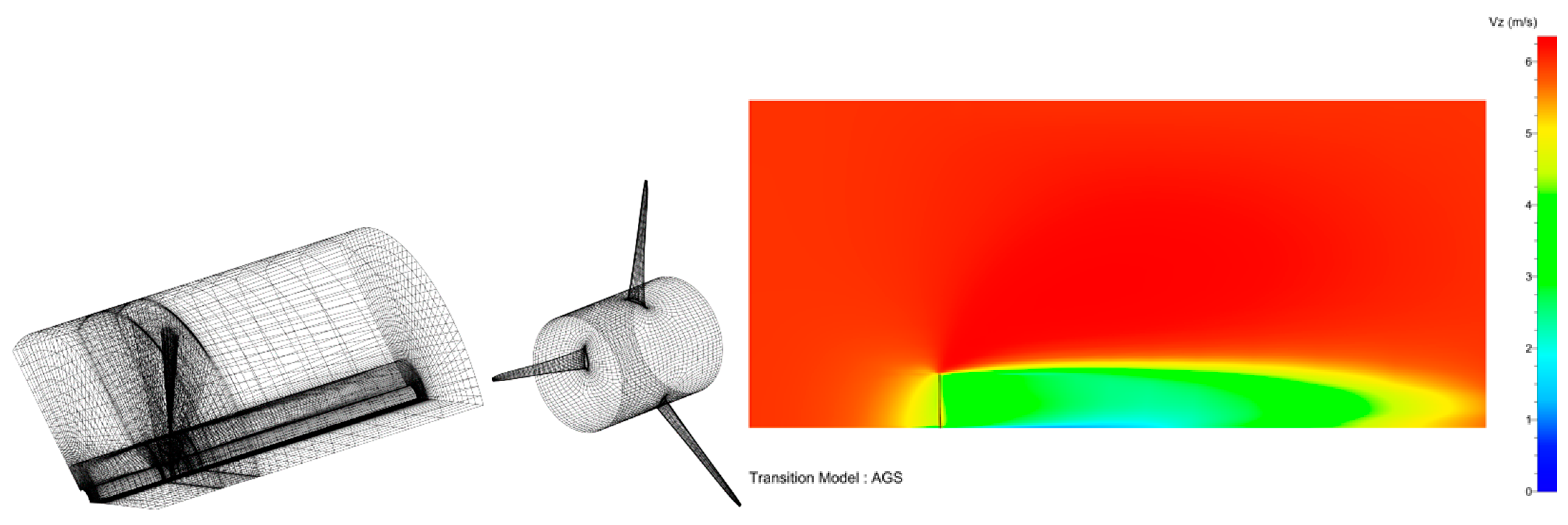
3.3.3. Hydrokinetic Turbine Rotor

A 3-bladed, 4 kW hydrokinetic turbine spinning at 2117 RPM, with an incoming velocity of 6 m/s, blade height of only 11 cm, and tip speed ratio of 6, is used for the one-way fluid–structure interaction demonstration. The 3D RANS solution of the blade is obtained to generate the pressure loads, and Figure 34 shows the periodic mesh used and Vz contour. The fluid domain includes sufficient upstream, free-stream, and downstream domains [62].

There is no inlet nor outlet boundary condition (BC) defined for unducted rotors. Instead, a free-stream domain is created and an external BC of atmospheric static pressure and temperature with an axial velocity of 6 m/s is defined with Spalart–Allmaras turbulence model. Figure 35 shows the structural analysis of the HKT rotor with stainless-steel as the material, and clearly, the stress is below the strength. A periodic domain was solved with nodes and tetrahedral elements. The aerodynamic loads affect the blade structure and a one-way FSI is required to design stronger blades, especially in denser fluids. The unidirectional fluid–structure interaction was performed using the ANSYS Mechanical solver using the pressure loads from FINE/Turbo mapped to the blade surface as shown in Figure 36. The stress is shown to be higher than the strength for the 4 kW HKT design case, which reveals that the chord near the hub must be much bigger and thicker sections need to be used to withstand those pressure loads. Better airfoil and chord definition are required to reduce the stress.

A SOGA-based optimization for maximum power generation using the above HKT design as a baseline is performed using the low-fidelity tool py_BEM, which defines spanwise properties and calculates efficiency based on the second law of thermodynamics [62]. Tip speed ratio, tip radius, 5 spanwise chord multiplier control points, and the blade count are varied, making a total of 8 parameters. 1200 function evaluations, a population size of 200 with 7 generations, 2 parents, and 2 offspring are initialized in the optimization cycle. Figure 37 shows the parameter variation at each evaluation and its efect on the performance with the optimum values, shown as black dots for each parameter. The tip loss function embedded in the py_BEM tool defines the performance loss near the tip and forces the optimizer to choose a smaller chord compared to other span locations. Total power generated by the HKT optimum is 18.6 kW, with 6 blades, a tip speed ratio of 6.8483, and a tip radius of 0.256 m. The coefficient of power is 0.8503, coefficient of thrust is 1.4048, and the second law efficiency (exergetic) is the ratio of these two coefficients and is calculated to be 60.39%.

4. Conclusions

A robust toolkit for multifidelity multidisciplinary design analysis and optimization of ducted and unducted turbomachinery using the DAKOTA package is described. Low-fidelity tools are connected to high-fidelity using the developed parametric blade geometry generator. A large design space is enabled for exploration through parameterization, definition of various objective functions, and constraints. Genetic algorithms and gradient methods are primarily used. Analysis at low fidelity is demonstrated using 0D, 1D, and 2D (quasi-3D) tools, resulting in optimum spanwise geometric properties. These properties become parametric inputs for the high-fidelity cycle incorporating automation chains and several developed data transfer tools. Smooth spanwise perturbations of geometric parameters such as metal angles, thickness, and curvature-driven meanline using B-spline control points generated non-intuitive optimums. The ability to create parametric 3D blade shapes quickly from low-fidelity analyses with advanced control is demonstrated to be unique and enables the rapid 3D design cycle. As part of the multidisciplinary analysis, 3D structural analysis is also performed through the unidirectional fluid–structure interaction for a few cases. It utilized spanwise pressure loads from the 3D RANS solver imported to 3D CAD in the FEA solver. Single- and multi-objective applications of the axial compressor rotor, compressor stage, axial turbine, radial compressor, diffuser, contra-rotating propeller, and wind and hydrokinetic turbines are demonstrated to prove the generality.

References

- Panchenko, Y.; Moustapha, H.; Mah, S.; Patel, K.; Dowhan, M.J.; Hall, D. Preliminary Multi-Disciplinary Optimization in Turbomachinery Design. In Proceedings of the RTO AVT Symposium on “Reduction of Military Vehicle Acquisition Time and Cost through Advanced Modelling and Virtual Simulation”, Paris, France, 22–25 April 2002. [Google Scholar]
- Pate, D.; Gray, J.S.; German, B. A Graph Theoretic Approach to Problem Formulation for Multidisciplinary Design Analysis and Optimization. Struct. Multidiscip. Optim. 2013, 51, 743–760. [Google Scholar] [CrossRef]
- Toal, D.J.J.; Keane, A.J.; Benito, D.; Dixon, J.A.; Yang, J.; Price, M.; Robinson, T.; Remouchamps, A.; Kill, N. Multi-Fidelity Multidisciplinary Whole Engine Thermo-Mechanical Design Optimization. J. Propuls. Power 2014, 30, 1654–1666. [Google Scholar] [CrossRef]
- Gray, J.S.; Hwang, J.T.; Martins, J.R.R.A.; Moore, K.T.; Naylor, B.A. OpenMDAO: An open-source framework for multidisciplinary design, analysis, and optimization. Struct. Multidiscip. Optim. 2019, 59, 1075–1104. [Google Scholar] [CrossRef]
- Sgueglia, A.; Schmollgruber, P.; Bartoli, N.; Benard, E.; Morlier, J.; Jasa, J.; Martins, J.R.R.A.; Hwang, J.T.; Gray, J.S. Multidisciplinary design optimization framework with coupled derivative computation for hybrid aircraft. J. Aircr. 2020, 57, 4. [Google Scholar] [CrossRef]
- Kontogiannis, S.G.; Savill, M.A. A generalized methodology for multidisciplinary design optimization using surrogate modelling and multifidelity analysis. Optim. Eng. 2021, 21, 723–759. [Google Scholar] [CrossRef]
- Dornberger, R.; Büche, D.; Stoll, P. Multidisciplinary optimization in turbomachinery design. In Proceedings of the European Congress on Computational Methods in Applied Sciences and Engineering, Barcelona, Spain, 11–14 September 2000. [Google Scholar]
- Kolonay, R.; Nagendra, S.; Laflen, J. Sensitivity analysis for turbine blade components. In Proceedings of the 40th Structures, Structural Dynamics, and Materials Conference and Exhibit, St. Louis, MO, USA, 12–15 April 1999. [Google Scholar]
- Xu, S.; Li, Y.; Huang, X.; Wang, D. Robust Newton–Krylov Adjoint Solver for the Sensitivity Analysis of Turbomachinery Aerodynamics. AIAA J. 2021, 59, 4014–4030. [Google Scholar] [CrossRef]
- McWilliam, M.K.; Dicholkar, A.C.; Zahle, F.; Kim, T. Post-Optimum Sensitivity Analysis with Automatically Tuned Numerical Gradients Applied to Swept Wind Turbine Blades. Energies 2022, 15, 2998. [Google Scholar] [CrossRef]
- Okui, H.; Verstraete, T.; den Braembussche, R.A.V.; Alsalihi, Z. Three-Dimensional Design and Optimization of a Transonic Rotor in Axial Flow Compressors. J. Turbomach. 2013, 135, 031009. [Google Scholar] [CrossRef]
- Eldred, M.S.; Adams, B.M.; Haskell, K.; Bohnhoff, W.J.; Eddy, J.P.; Gay, D.M.; Hart, W.E.; Hough, P.D.; Kolda, T.G.; Swiler, L.P.; et al. DAKOTA Reference Manual, 4.2 ed.; Sandia National Laboratories: Albuquerque, NM, USA, 2008. [Google Scholar]
- Kipouros, T.; Jaeggi, D.; Dawes, B.; Parks, G.; Savill, M. Multi-objective optimisation of turbomachinery blades using Tabu search. In Proceedings of the Evolutionary Multi-Criterion Optimization: Third International Conference, EMO 2005, Guanajuato, Mexico, 9–11 March 2005; Lecture Notes in Computer Science. Springer: Berlin/Heidelberg, Germany, 2005; Volume 3410, pp. 897–910. [Google Scholar]
- Kipouros, T.; Jaeggi, D.M.; Dawes, W.N.; Parks, G.T.; Savill, A.M.; Clarkson, P.J. Biobjective design optimization for axial compressors using tabu search. AIAA J. 2008, 46, 701–711. [Google Scholar] [CrossRef]
- Samareh, J. Survey of shape parameterization techniques for high-fidelity multidisciplinary shape optimization. AIAA J. 2001, 39, 877–884. [Google Scholar] [CrossRef]
- Sripawadkul, V.; Padulo, M.; Guenov, M. A comparison of airfoil shape parameterization techniques for early design optimization. In Proceedings of the 13th AIAA/ISSMO Multidisciplinary Analysis and Optimization Conference 2010, Ft. Worth, TX, USA, 13–15 September 2010. [Google Scholar]
- Sobester, A.; Barretty, T. The quest for a truly parsimonious airfoil parameterization scheme. In Proceedings of the 8th AIAA Aviation Technology, Integration and Operations (ATIO) Conference, Anchorage, AL USA, 14–19 September 2008. [Google Scholar]
- Castonguay, P.; Nadarajah, S. Effect of shape parameterization on aerodynamic shape optimization. In Collection of Technical Papers—45th AIAA Aerospace Sciences Meeting; American Institute of Aeronautics and Astronautics: Washington, DC, USA, 2007; Volume 1, pp. 561–580. [Google Scholar]
- Mousavi, A.; Castonguay, P.; Nadarajah, S. Survey of shape parameterization techniques and its effect on three-dimensional aerodynamic shape optimization. In Proceedings of the Collection of Technical Papers—18th AIAA Computational Fluid Dynamics Conference, Miami, FL, USA, 25–28 June 2007; Volume 1, pp. 234–254. [Google Scholar]
- He, Y.; Agarwal, R. Shape optimization of NREL s809 airfoil for wind turbine blades using a multi-objective genetic algorithm. Int. J. Aerosp. Eng. 2014, 2014, 864210. [Google Scholar] [CrossRef]
- Bhide, K.R. Shock Boundary Layer Interactions—A Multiphysics Approach. Master’s Thesis, University of Cincinnati, Cincinnati, OH, USA, 2018. [Google Scholar]
- Bhide, K.; Siddappaji, K.; Abdallah, S. Influence of fluid–thermal–structural interaction on boundary layer flow in rectangular supersonic nozzles. Aerospace 2018, 5, 33. [Google Scholar] [CrossRef]
- ANSYS. Available online: www.ansys.com (accessed on 24 December 2020).
- Pierret, S.; Kato, H.; Coelho, R.F.; Merchant, A. Aero-mechanical optimization method with direct cad access: Application to counter rotating fan design. ASME Turbo Expo 2006, 2006, 1329–1341. [Google Scholar]
- Van den Braembussche, R.A. Numerical Optimization for Advanced Turbomachinery Design in Optimization and Computational Fluid Dynamics; Springer: Berlin/Heidelberg, Germany, 2008; Part II; pp. 147–189. ISBN 978-3-540-72152-9. [Google Scholar]
- Grasel, J.; Keskin, A.; Swoboda, M.; Przewozny, H.; Saxer, A. A full parametric model for turbomachinery blade design and optimization. In Proceedings of the International Design Engineering Technical Conference & Computers and Information in Engineering, Salt Lake City, UT, USA, 28 September–2 October 2004. [Google Scholar]
- Demeulenaere, A.; Purwanto, A.; Ligout, A.; Hirsch, C. Design and Optimization of an Industrial Pump: Application of Genetic Algorithms and Neural Network; ASME FEDSM2005-77487; ASME: New York, NY, USA, 2005. [Google Scholar]
- Demeulenaere, A.; LigoutI, A.; Hirsch, C. Application of Multipoint Optimization to the Design of Turbomachinery Blades; ASME GT2004-53110; ASME: New York, NY, USA, 2004. [Google Scholar]
- Chen, J.; Liu, C.; Xuan, L.; Zhang, Z.; Zou, Z. Knowledge-based turbomachinery design system via a deep neural network and multi-output Gaussian process. Knowl.-Based Syst. 2022, 252, 109352. [Google Scholar] [CrossRef]
- Luo, J.; Chen, Z.; Zheng, Y. A gradient-based method assisted by surrogate model for robust optimization of turbomachinery blades. Chin. J. Aeronaut. 2021, in press. [Google Scholar] [CrossRef]
- Staubach, J.B. Multidisciplinary Design Optimization, MDO, the Next Frontier of CAD/CAE in the Design of Aircraft Propulsion Systems; AIAA Paper; AIAA: Dayton, OH, USA, 2003; pp. 2003–2803. [Google Scholar]
- Benini, E. Three-Dimensional Multi-Objective Design Optimization of a Transonic Compressor Rotor. J. Propuls. Power 2004, 20, 559–565. [Google Scholar] [CrossRef]
- Oyama, A.; Liou, M.S.; Obayashi, S. Transonic Axial Flow Blade Optimization Evolutionary Algorithms Three-Dimensional Navier Stokes Solver. J. Propuls. Power 2004, 20, 612–619. [Google Scholar] [CrossRef]
- Jang, C.-M.; Li, P.; Kim, K.Y. Optimization of Blade Sweep in a transonic Axial Compressor Rotor. JSME Int. J. 2005, 48, 793–801. [Google Scholar] [CrossRef]
- Lian, Y.; Liou, M.S. Multi-Objective Optimization of Transonic Compressor Blade Using Evolutionary Algorithm. J. Propuls. Power 2005, 21, 979–987. [Google Scholar] [CrossRef]
- Koch, C.C. Stalling Pressure Rise Capability of Axial Flow Compressor Stages. J. Eng. Power 1981, 103, 645–656. [Google Scholar] [CrossRef]
- Nemnem, A.F. A General Multidisciplinary Turbomachinery Design Optimization System Applied to a Transonic Fan. Ph.D. Dissertation, University of Cincinnati, Cincinnati, OH, USA, 2014. [Google Scholar]
- James, A.; Jones, J. A Multidisciplinary Algorithm for the 3-d Design Optimization of Transonic Axial Compressor Blades. Ph.D. Thesis, Naval Postgraduate School, Monterey, CA, USA, June 2002. [Google Scholar]
- Ellbrant, L.; Eriksson, L.E.; Martensson, H. Design of Compressor Blades considering Efficiency and Stability using CFD based Optimization. ASME Turbo Expo 2012, 44748, 371–382. [Google Scholar]
- Ellbrant, L.; Eriksson, L.E.; Martensson, H. Balancing efficiency and stability in the design of transonic compressor stages. In Proceedings of the ASME Turbo Expo 2013: Turbine Technical Conference and Exposition, San Antonio, TX, USA, 3–7 June 2013. [Google Scholar]
- Siller, U.; Vob, C.; Nicke, E. Automated Multidisciplinary Optimization of a Transonic Axial Compressor. In Proceedings of the 47th AIAA Aerospace Sciences Meeting Including the New Horizons Forum and Aerospace Exposition, Orlando, FL, USA, 5–8 January 2009. [Google Scholar]
- Deng, X.; Guo, F.; Liu, Y.; Han, P. Aero-mechanical optimization design of a transonic fan blade. In Proceedings of the ASME Turbo Expo 2013: Turbine Technical Conference and Exposition, San Antonio, TX, USA, 3–7 June 2013. [Google Scholar]
- Siller, U.; Aulich, M. Multidisciplinary 3d-Optimization of a Fan Stage Performance Map with Consideration of the Static and Dynamic Rotor Mechanics; GT2010-22792; ASME: New York, NY, USA, 2010. [Google Scholar]
- Vob, C.; Aulich, M.; Kaplan, B.; Nicke, E. Automated multiobjective optimisation in axial compressor blade design. ASME Turbo Expo 2006, 55232, V06BT43A014. [Google Scholar]
- Joly, M.; Verstraete, T.; Paniagua, G. Full design of a highly loaded and compact contra-rotating fan using multidisciplinary evolutionary optimization. ASME Turbo Expo 2013, 55232, V06BT43A009. [Google Scholar]
- Braembussche, R.; Alsalihi, Z.; Verstraete, T.; Matsuo, A.; Seiichi, I.; Sugimoto, K.; Isao, T. Multidisciplinary Multipoint Optimization of a Transonic Turbocharger Compressor. Proc. ASME Turbo Expo 2008, 44748, 903–913. [Google Scholar]
- Ceyhan, O. Aerodynamic design and optimization of horizontal axis wind turbines by using bem theory and genetic algorithm. In Praca Magisterska; Middle East Technical University: Ankara, Turkey, 2008. [Google Scholar]
- Kolekar, N.; Hu, Z.; Banerjee, A.; Du, X. Hydrodynamic design and optimization of hydro-kinetic turbines using a robust design method. In Proceedings of the 1st Marine Energy Technology Symposium, Washington, DC, USA, 10–11 April 2013. [Google Scholar]
- Bhide, K.; Siddappaji, K.; Abdallah, S.; Roberts, K. Improved Supersonic Turbulent Flow Characteristics Using Non-Linear Eddy Viscosity Relation in RANS and HPC-Enabled LES. Aerospace 2021, 8, 352. [Google Scholar] [CrossRef]
- Bhide, K.R.; Abdallah, S. Turbulence statistics of supersonic rectangular jets using Reynolds Stress Model in RANS and WALE LES. In AIAA AVIATION 2022 Forum; AIAA: Chicago, IL, USA, 2022. [Google Scholar]
- Bhide, K.; Abdallah, S. Anisotropic Turbulent Kinetic Energy Budgets in Compressible Rectangular Jets. Aerospace 2022, 9, 484. [Google Scholar] [CrossRef]
- Bhide, K. Supersonic retro propulsion: Aero-thermal-structural analysis. In Proceedings of the International Conference of Jets, Wakes, Separated Flows (ICJWSF), Tokyo, Japan, 7 March 2022. [Google Scholar]
- Turner, M.G.; Bruna, D.; Merchant, A. Applications of a turbomachinery design tool for compressors and turbines. In Proceedings of the 43rd AIAA/ASME/SAE/ASEE Joint Propulsion Conference & Exhibit, Cincinnati, OH, USA, 8–11 July 2007. [Google Scholar] [CrossRef]
- Gutzwiller, D.P. Automated design, analysis, and optimization of turbomachinery disks. Master’s Thesis, University of Cincinnati, Cincinnati, OH, USA, September 2009. [Google Scholar]
- Gutzwiller, D.P.; Turner, M.G.; Downing, M.J. Educational software for blade and disk design. ASME Turbo Expo 2009, 48821, 827–838. [Google Scholar]
- Muppana, S. Multi-fidelity Design and Analysis of Single Hub Multi-Rotor High Pressure Centrifugal Compressor. Master’s Thesis, University of Cincinnati, Cincinnati, OH, USA, 2018. [Google Scholar]
- Mishra, S. Developing Novel Computational Fluid Dynamics Technique for Incompressible Flow and Flow Path Design of Novel Centrifugal Compressor. Master’s Thesis, University of Cincinnati, Cincinnati, OH, USA, 2016. [Google Scholar]
- Qiu, X.; Mallikarachchi, C.; Anderson, M. A new slip factor model for axial and radial impellers. In Proceedings of the ASME Turbo Expo 2007: Power for Land, Sea, and Air, Montreal, QC, Canada, 14–17 May 2007. [Google Scholar]
- Drela, M. A User Guide for MISES 2.53; Technical Report; MIT Computational Science Laboratory: Cambridge, MA, USA, 1998; Volume 47950, pp. 957–966. [Google Scholar]
- Cherry, D.G.; Lenahan, D.T. Energy Efficient Engine. Low Pressure Turbine Test Hardware Detailed Design Report. NASA CR 1982, 167956, G3/07 24804. Available online: https://ntrs.nasa.gov/citations/19850002686 (accessed on 20 August 2022).
- Siddappaji, K. Parametric 3d blade geometry modeling tool for turbomachinery systems. Master’s Thesis, University of Cincinnati, Cincinnati, OH, USA, 2012. [Google Scholar]
- Siddappaji, K. On the Entropy Rise in General Unducted Rotors Using Momentum, Vorticity and Energy Transport. Doctoral Dissertation, University of Cincinnati, Cincinnati, OH, USA, 2018. [Google Scholar]
- Drela, M. XFOIL: An Analysis and Design System for Low Reynolds Number Airfoils; Springer: Heidelberg/Berlin, Germany, 1989. [Google Scholar]
- Fineturbo/Autogrid, NUMECA International. Available online: https://www.numeca.com (accessed on 24 December 2020).
- Siddappaji, K.; Turner, M.G. Versatile Tool for Parametric Smooth Turbomachinery Blades. Aerospace 2022, 9, 489. [Google Scholar] [CrossRef]
- Park, K.; Turner, M.G.; Siddappaji, K.; Dey, S.; Merchant, A. Optimization of a 3-Stage Booster Part 1: The Axisymmetric Multidisciplinary Optimization Approach to Compressor Design; ASME Paper Number GT2011-46569; ASME: New York, NY, USA, 2011. [Google Scholar]
- Holloway, P.R.; Knight, G.L.; Koch, C.C.; Shaffer, S.J. Energy Efficient Engine High Pressure Compressor Detail Design Report; Technical Report; NASA-CR-165558; General Electric Company: Boston, MA, USA, 1982. [Google Scholar]
- Mahmood, S.M.H.; Turner, M.G.; Siddappaji, K.; Balasubramanian, K. Flow Characteristics of an Optimized Axial Compressor Rotor using Smooth Design Parameters. In Proceedings of the ASME Turbo Expo 2016: Turbomachinery Technical Conference and Exposition, Seoul, Korea, 13–17 June 2016. [Google Scholar]
- Chen, H.; Turner, M.G.; Siddappaji, K.; Mahmood, S.M.H. Vorticity dynamics-based flow diagnosis for a 1.5-stage high pressure compressor with an optimized transonic rotor. In Proceedings of the ASME Turbo Expo 2016: Turbomachinery Technical Conference and Exposition, Seoul, Korea, 13–17 June 2016. [Google Scholar]
- Somtrakool, S. Automated Campbell Diagram Module on Optimization of Transonic Fan. Master’s Thesis, University of Cincinnati, Cincinnati, OH, USA, 2014. [Google Scholar]
- Gunn, E.J.; Hall, C.A. Aerodynamic of Boundary Layer Ingesting Fans. In Proceedings of the ASME Turbo Expo 2014: Turbine Technical Conference and Exposition, GT2014-26142, Dusseldorf, Germany, 16–20 June 2014. [Google Scholar]
- Gunn., E.J.; Hall, C.A. Non-Axisymmetric Stator Design for Boundary Layer Ingesting Fans. In Proceedings of the ASME Turbo Expo 2017, Charlotte, NC, USA, 26–30 June 2017. GT2017-63082. [Google Scholar]
- Kumar, S.; Siddappaji, K.; Turner, M.G.; Celestina, M. Aerodynamic design system for non-axisymmetric boundary layer ingestion fans. ASME Turbo Expo 2018, 51012, V02CT42A048. [Google Scholar]
- Denton, J.D. Loss Mechanisms in Turbomachines. ASME J. Turbomach. 1993, 115, 621–656. [Google Scholar] [CrossRef]
- Smith, J.; Leroy, H.; Yeh, H. Sweep and Dihedral Effects in Axial-Flow Turbomachinery. J. ASME 1963, 85, 401–414. [Google Scholar] [CrossRef]
- JetCAT. Available online: https://www.jetcat.de/en/products/ (accessed on 24 December 2012).
- SolidConcepts. Available online: https://solidconceptsnc.com/ (accessed on 24 December 2012).
- Krain, H. Swirling impeller flow. J. Turbomach. 1988, 110, 122–128. [Google Scholar] [CrossRef]
- Hathaway, M.D. Laser anemometer measurements of the three-dimensional rotor flow field in the NASA low speed centrifugal compressor. Tech. Rep. 1995, 60, 3527, ARL-TR-333. Available online: https://www.researchgate.net/publication/24286133_Laser_anemometer_measurements_of_the_three-dimensional_rotor_flow_field_in_the_NASA_low-speed_centrifugal_compressor (accessed on 20 August 2022).
- Sato, K.; He, L. Effect of rotor-stator interaction on impeller performance in centrifugal compressors. Int. J. Rotating Mach. 1999, 5, 135–146. [Google Scholar] [CrossRef] [Green Version]
- Shaaban, A. Fluid Flow Controller Us Patent. 6589013 b2, 2001. [Google Scholar]
- Holden, J.R.; Caley, T.M.; Heberling, B.; Cantor, C.; Wesseling, E.; Hamed, A.A.; Turner, M.G.; Litke, P.J.; Grannan, N.D. Novel Design and Fabrication of JetCat P90 Diffuser using Parametric Design and Optimization Tools. In Proceedings of the AIAA 2016-2128—54th AIAA Aerospace Sciences Meeting, San Diego, CA, USA, 4–8 January 2016. [Google Scholar]
- Feldhacker, J.; Staikoff, N.; Schwartzwalder, R.; Mitchell, F.; Hoffmann, D.; Begovich, M. A research paper on redesigning the compressor diffuser of a jetcat P90 turbine to improve the efficiency. In APOP 2015, Technical Report; University of Cincinnati: Cincinnati, OH, USA, 2015. [Google Scholar]
- Dey, S. Wind turbine blade design system, aerodynamic and structural analysis. Master’s Thesis, University of Cincinnati, Cincinnati, OH, USA, 2011. [Google Scholar]
- Balasubramanian, K. Novel, Unified, Curvature-Based Airfoil Parameterization Model for Turbomachinery Blades and Wings. Master’s Thesis, University of Cincinnati, Cincinnati, OH, USA, 2018. [Google Scholar]
- Giguere, P.; Selig, M. Design of a tapered and twisted blade for the nrel combined experiment rotor. In Technical Report NREL/SR-500-26173; NREL: Golden, CO, USA, 1999. [Google Scholar]
Publisher’s Note: MDPI stays neutral with regard to jurisdictional claims in published maps and institutional affiliations. |
© 2022 by the authors. Licensee MDPI, Basel, Switzerland. This article is an open access article distributed under the terms and conditions of the Creative Commons Attribution (CC BY) license (https://creativecommons.org/licenses/by/4.0/).
Share and Cite
Siddappaji, K.; Turner, M.G. An Advanced Multifidelity Multidisciplinary Design Analysis Optimization Toolkit for General Turbomachinery. Processes 2022, 10, 1845. https://doi.org/10.3390/pr10091845
Siddappaji K, Turner MG. An Advanced Multifidelity Multidisciplinary Design Analysis Optimization Toolkit for General Turbomachinery. Processes. 2022; 10(9):1845. https://doi.org/10.3390/pr10091845
Chicago/Turabian StyleSiddappaji, Kiran, and Mark G. Turner. 2022. "An Advanced Multifidelity Multidisciplinary Design Analysis Optimization Toolkit for General Turbomachinery" Processes 10, no. 9: 1845. https://doi.org/10.3390/pr10091845
APA StyleSiddappaji, K., & Turner, M. G. (2022). An Advanced Multifidelity Multidisciplinary Design Analysis Optimization Toolkit for General Turbomachinery. Processes, 10(9), 1845. https://doi.org/10.3390/pr10091845