Performance Analysis of Energy Production of Large-Scale Solar Plants Based on Artificial Intelligence (Machine Learning) Technique

Abstract

Due to the continual fusion reaction, the sun generates tremendous energy. This solar energy is freely available and can be extracted by installing a large-scale solar power plant. Therefore, such PV solar plants are key contributors to cutting the energy deficit in remote areas. This study focused on predicting a 10-year performance analysis of a large-scale solar power plant by using 1 year of real-time data from the Quaid-e-Azam Solar Park (QASP) situated in Bahawalpur, Pakistan. For the purpose of prediction, the ARIMA model was developed using Python, which is one of the best tools in machine learning. Since ARIMA is a statistical technique for prediction, by using the developed model through Python, we predicted the values of the performance ratio (PR), production amount (MWh), and plan of array (POA) of the solar plant for the next 10 years using 1 year of real-time data. This machine learning prediction technique is very effective and efficient, compared with other traditional prediction and forecasting techniques, for estimating the performance of the solar power plant and the status of the solar power plant in the long-term future. The forecasting/prediction results acquired from the process show that power production during the next ten years increases to approximately 400 MW and that POA will grow from 6.8 to 7.8 W/m². However, a decline occurred in the performance ratio, which decreased from 76.7% to 73%. Based on these results, the ARIMA model for predicting solar power generation is effective and can be utilized for any solar power plant.

1. Introduction

Due to continuous fusion reaction, the sun is a superabundant and permanent energy source. On earth, solar power panels consume a limited amount of their energy through photovoltaic technology. This technology plays an important role in responding to global warming and meeting future energy demands. In addition to its zero emissions profile, solar energy minimizes carbon footprints by directly contributing to the reduction of greenhouse gas emissions [1,2]. In recent years, the solar energy sector has set new records for electricity production and aims to reduce the usage of fossil fuels as these are shrinking daily and may diminish over time [3]. In addition, solar energy minimizes grid load and increases power access to remote areas in developing countries. Improving the efficiency of solar energy systems with the help of emerging technologies is an important study for developing this sector. However, a PV system’s effectiveness is affected by various variables, including weather, lighting, energy loss of several types, system corrosion over time, etc. Almost 19 MJ/m² of solar energy is received each day, while the amount of solar power produced is 5.3 kWh/m²/day [4].

Pakistan’s total land area is almost 796,096 km². It is the 33rd largest country in the world by area, having a population of 227 million, and it has great potential for creating solar power. However, just 0.071% of the country’s land is being utilized to fulfill Pakistan’s current energy consumption, as reported by the World Bank. The region of Pakistan has some of the highest insulation levels in the world and receives eight to nine hours of sunlight per day, which is excellent for producing solar power. The country has solar plants in the Punjab, Sindh, and Balochistan provinces. The first use of this technology in Pakistan was on 29 May 2015 in Islamabad, and the project title was “Introduction of Clean Energy by Solar Electricity Generation System.” This project was aided by the Japan International Cooperation Agency (JICA) [5]. Now, Pakistan has the largest solar power park in Bahawalpur, a city of Punjab, which tends to generate 100 megawatts of electricity and which will reach 1000 megawatts in the future. The solar radiation, surrounding temperature, weather, and geographic location significantly impact PV panels [6]. In addition, energy operators must balance electricity consumption and generation to save electricity generated by renewable power plants and avoid losses. In addition, consumers must be able to access sufficient power. As a result, the grid-connection of solar plants is something the renewable energy sector is moving toward. The major issue this sector is facing is network instability [7]. To plan for the future, it is vital to anticipate how much electricity will be produced by solar plants in particular and renewable energy farms in general [8,9]. Therefore, being able to forecast the volume of photovoltaic installations that will be made in the upcoming days is crucial. Quaid-e-Azam Solar Park is Pakistan’s first significant solar power project [4,10]. It is generating 400 MW and will be extended to 1000 MW in the future. To proceed further, there is a need to discuss the feasibility of and future predictions about the power generation of this huge project.

Some comparative studies related to solar energy prediction/forecast are already published. Haoyin Ye et al. [11] explained the state-of-the-art potential issues and the challenges of solar energy based on a forecasting approach. The current PV prediction methods are widely split into three categories: statistical, physical, and forecasting technologies associated with artificial intelligence and based on the long-term modeling of forecast/prediction [12]. Pedro and Coimbra et al. [13] used the ARIMA model to predict the production of a 1 MW PV solar plant. Another study was based on the literature of the SARIMA model, which performed the solar prediction of solar plants [14]. Li et al. [15] applied the support vector machine (SVM) technique to build a regression-algorithm prediction model for large-scale solar plants. Zhu et al. [16] employed the least squares support vector machine (LSSVM) to predict the power generation of the solar plant. Waqas et al. [17] used deep learning-based ensemble-stacking techniques to forecast solar energy production. In addition, many machine learning-based forecasting approaches for solar plants were proposed in the literature [18,19,20]. However, to address these issues of providing accurate solar plant prediction and forecast trends, extensive research studies [21,22,23] were recently conducted. In our study, a prediction method was adopted to identify how this solar plant will work in the future, i.e., after 10 years, whether or not it would be able to generate electricity. Through artificial intelligence and machine learning techniques, this prediction was made. For this purpose, the ARIMA model was used since it is a statistical prediction model that is very effective and efficient compared with other traditional methods.

2. Materials and Methods

The ARIMA technique used in this study makes use of time series data to forecast trends and to better understand the data set [24]. First, the developed model was trained using one year of real-time data acquired by QASP. Second, one-year prediction results were identified and are visualized in graphical form. Finally, using the predicted results from the machine learning process using the ARIMA model, 10 years of predictions were generated, encompassing 2020 through 2029. Real-time data was collected from the Quaid-e-Azam Solar Park from 2018 through 2019.

Several factors are considered when choosing a site for a solar PV project. These include the availability of unused land, high insulation, and clear skies all year long; the site of the QASP, as explained in [25], satisfies most of the prerequisites for producing electric power using PV technology. A comparative study of the energetic performance of a solar PV module was done in [26]. The performance analysis of a grid-connected solar project in a specific region was examined in [27]. We also found another performance study conducted based on the investigation of the performance of a grid-connected solar project in the Morocco region [28]. Similarly, a feasibility study of a 1 MW grid-connected techno-economic solution was done in Oman [29]. A study of the cost analysis of large-size solar projects was investigated in desert areas and shows the cost-effectiveness and advantages of solar performance [30]. The above was studied and examined in the PV domain as a model approach for judging the performance of the solar system in specific sizes and regions. Figure 1 shows the view of Quaid-e-Azam Solar Park, which is located in Bahawalpur, Pakistan. Due to its location in Pakistan’s largest desert and since most of its land is uncultivated and barren, the park satisfies all of these requirements. This solar plant was installed as part of the Renewable Energy Policy of 2006 [31]. The initial capacity of this solar plant is 100 MW, which will be upgraded by 20% in 2025 and by 30% in 2030. We collected data from this solar plant to get true and real-time values of parameters such as MWh (energy production), POA (plane of array), and PR (performance ratio).

Figure 2 shows the structural diagram of QASP, in which standard testing condition results are mentioned along with average solar plant performance. Figure 2 also shows that under STC, the solar plant runs at 80% efficiency in delivering power to the national grid.

The following are important contributions by our study for predicting future trends in solar energy:

(i).

The technical overview and explanation of the 100 MW solar project location and size and the solar plant structure.

(ii).

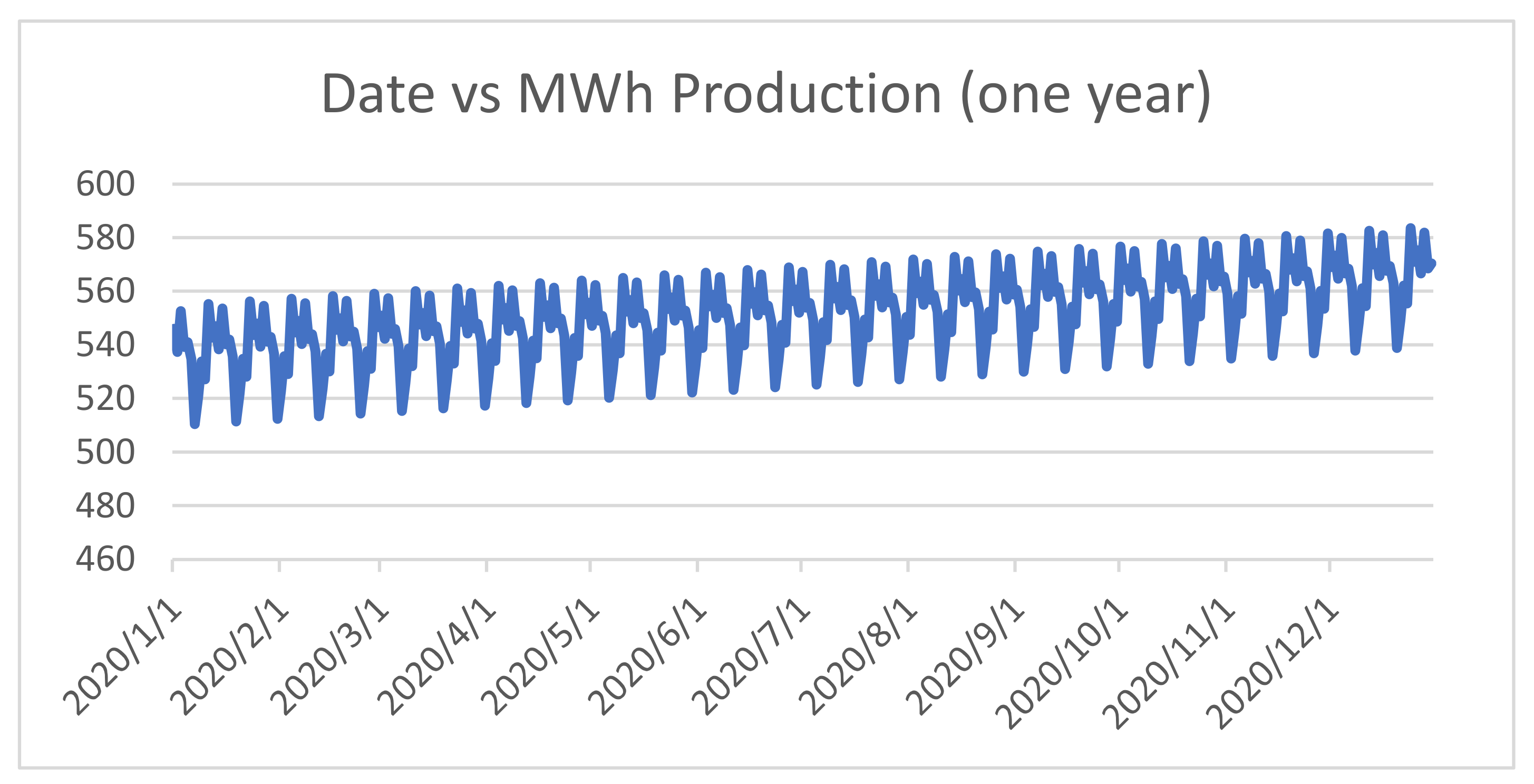
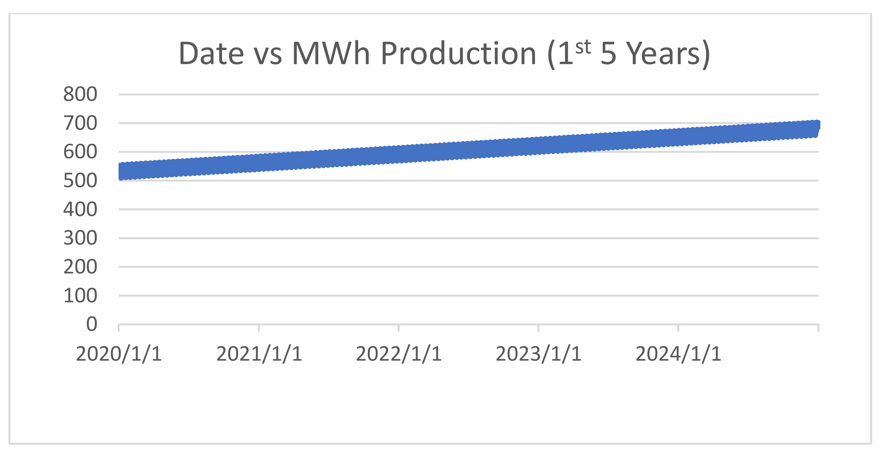
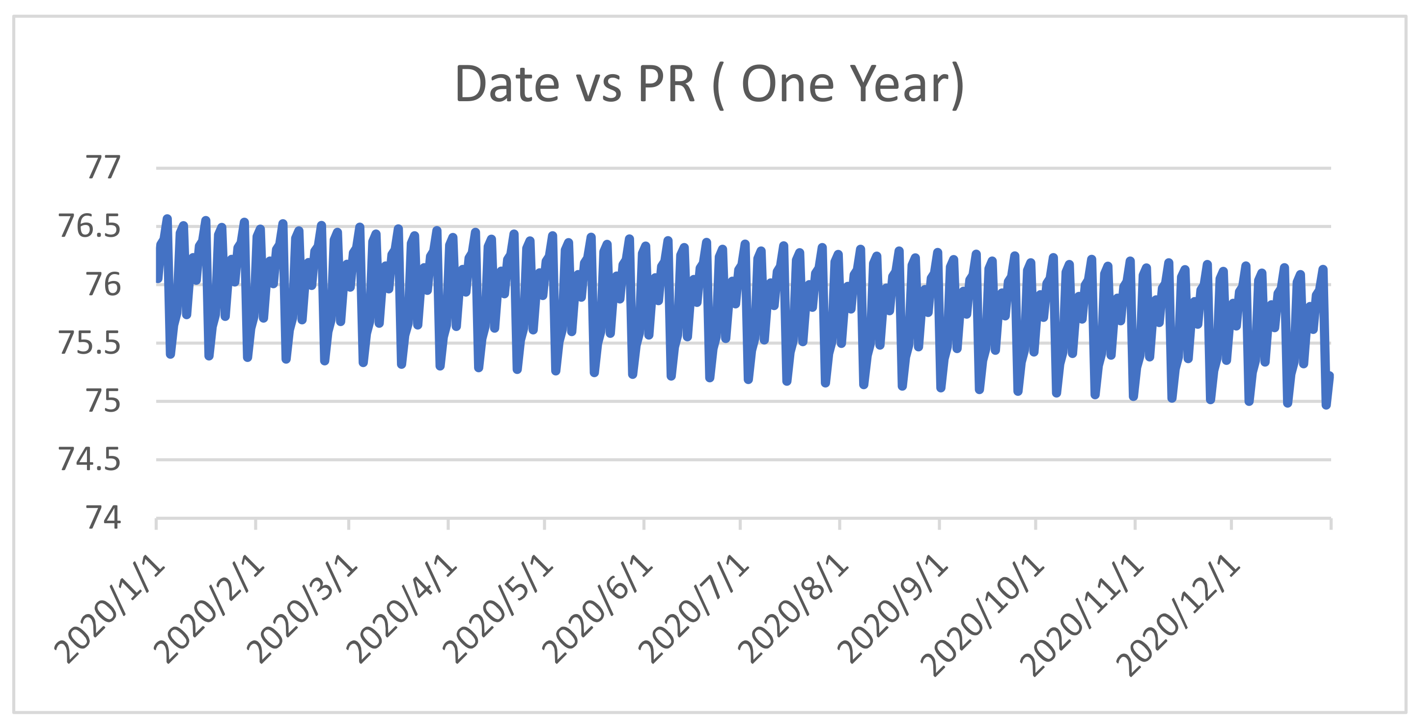
One year of real-time data was compiled from the 100 MW solar project for the purpose of analyzing the future performance predictions of solar production.

(iii).

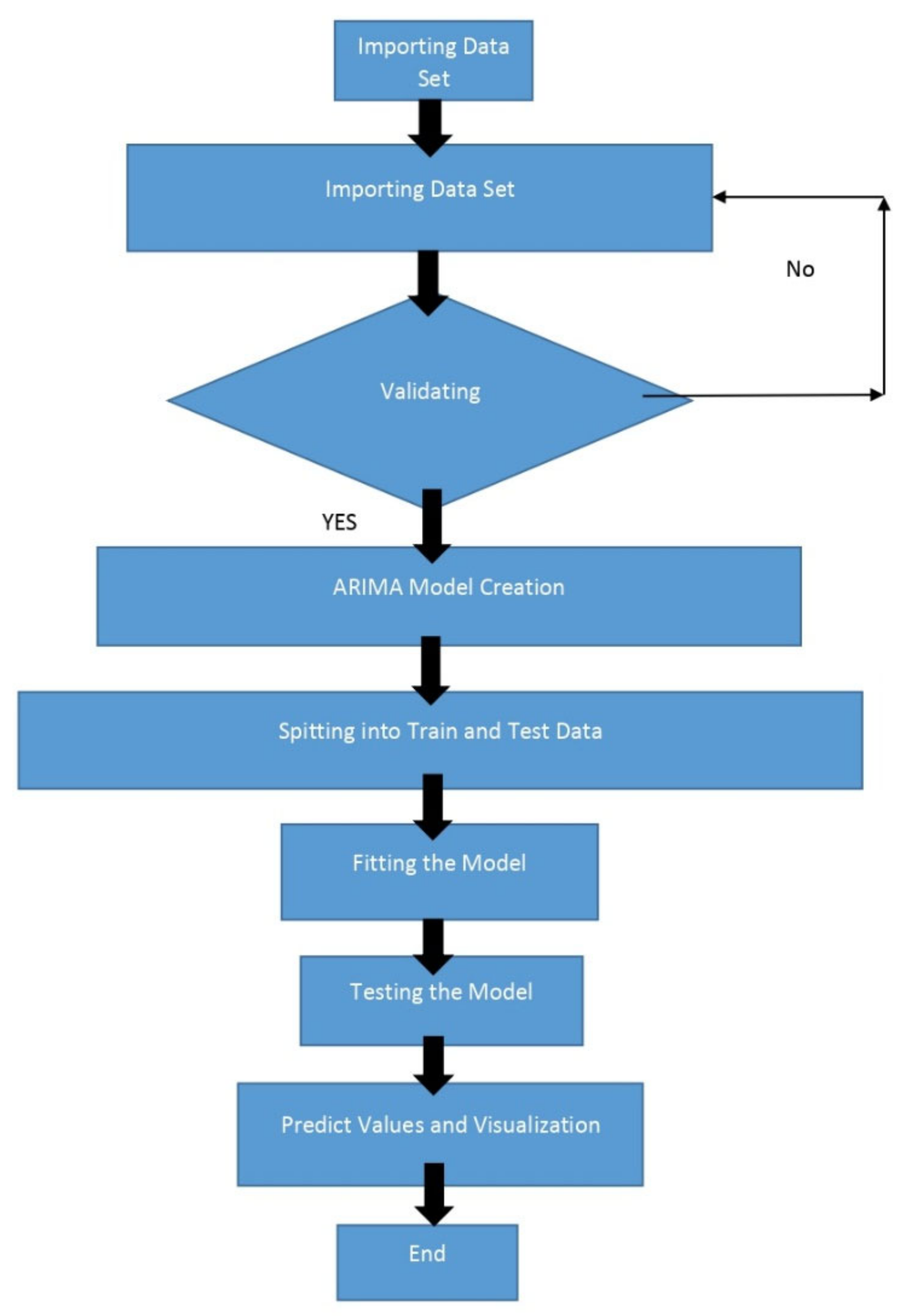
For forecasting future trends, the 1-year real-time data was incorporated through the ARIMA model and used for the forecasting techniques.

(iv).

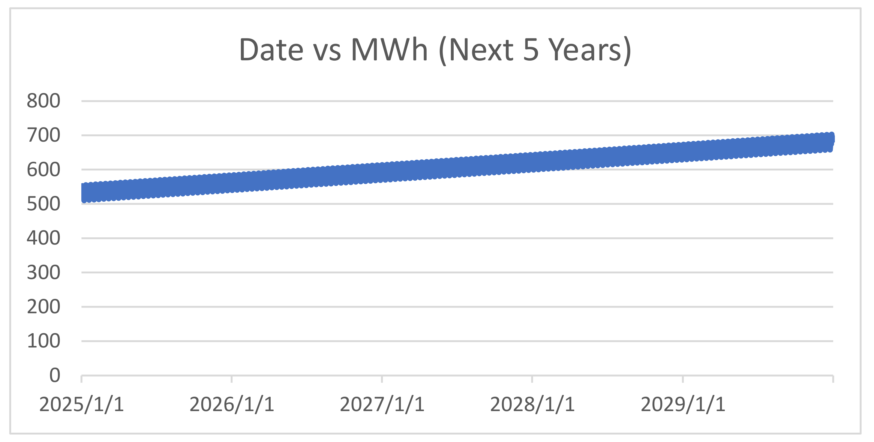
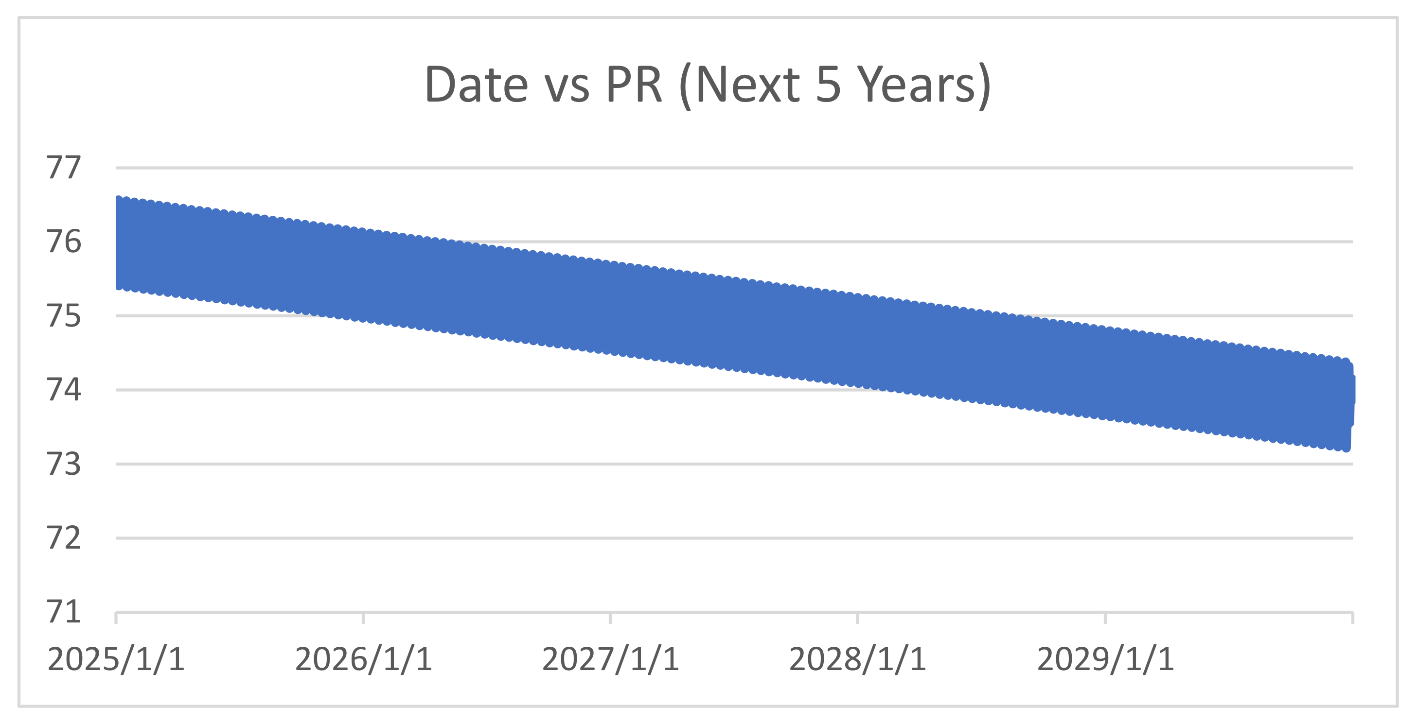
The ARIMA model was developed through machine learning techniques, and the model was trained to forecast the amount of solar energy.

(v).

The forecast/prediction results were visualized in graphical form through the machine learning process by using our developed ARIMA model.

Table 1. Technical description of the solar plant.

Detail of Equipment	No.	Units
Substation type	1	AIS
Installed capacity	100	MW
PV panel	392,160	225 Wp
Box of combiner	1300	DC
PV inverter	200	500 Kw
Auxiliary transformer	100	0.315/33 kV
Feeder	20	33 kV collection system loop
Main transformer	02	132 kVA to 100 MVA
SVC	02	−5~+15 MVAR

shows the details of the major equipment installed for the solar plant, having a power generation capacity of 100 MW.

2.1. Mathematical Expression for ARIMA

Forecast prediction is important in order to achieve the best results in any project or business. The tools and ideas behind time series forecasting are applicable to many businesses, not just to those that produce electricity [32]. ARIMA (Autoregressive Integrated Moving Average) [14] is the forecasting analysis technique that can predict future values using past values. This model is characterized by three parameters: p, q, and d, i.e., order of AR term (p), order of MA term (q) and the difference (d) needed to build the stationary time series.

By subtracting the previous values from the current values, which should be the minimum value, a time series can be made stationary in order to build ARIMA models, since a term AR (p) is a linear regression model that uses its own lags as prediction [33,34].

$$Y_t={\beta }_1{y}_{t-1}+{\beta }_2{y}_{t-2}+\cdots +{\beta }_0{y}_0+{\mathsf{\varepsilon }}_t$$

(1)

$$Y_{t-1}={\beta }_1{y}_{t-2}+{\beta }_2{y}_{t-3}+\cdots +{\beta }_0{y}_0+{\mathsf{\varepsilon }}_{t-1}$$

(2)

A pure AR model is one in which $Y_t$ depends upon its own lags.

$$Y_t={\beta }_1{y}_{t-1}+{\beta }_2{y}_{t-2}+\cdots +{\beta }_0{y}_0+{\mathsf{\varepsilon }}_t$$

(3)

Likewise, an MA (q) model is one where $Y_t$ depends only on the lagged forecast errors. By finding the values of the parameters p, q, and d, an ARIMA model can be created as follows using the stats model’s library [33,34]:

$$Y_t=\alpha +{\epsilon }_t+{\varnothing }_1{\epsilon }_{t-1}+{\varnothing }_2{\epsilon }_{t-2}+\cdots +{\varnothing }_q{\epsilon }_{t-q}$$

(4)

Here, the error terms are the errors of the autoregressive models of the respective lags. The errors ${\epsilon }_t$ and ${\epsilon }_{t-1}$ are the errors from Equations (2) and (3). The above-mentioned models are AR (p) and MA (q) models, respectively, but the real ARIMA model is one where the time series is differenced (d) at least one to make it stationary. By combining the AR (p) and MA (q) terms together, we find the following equation [33,34].

$$Y_t=\alpha +{\beta }_1{y}_{t-1}+{\beta }_2{y}_{t-2}+{\beta }_p{y}_{t-p}{\epsilon }_t+{\varnothing }_1{\epsilon }_{t-1}+{\varnothing }_2{\epsilon }_{t-2}\cdots +{\varnothing }_q{\epsilon }_{t-q}$$

(5)

where t is the number of terms, $Y_t$ is the function of the lags of $Y_t$, $\alpha$ is the intercept term, $\beta$ is the coefficient of the lag, ${\epsilon }_t$ is the lag forecast error, and φ is the coefficient of the lag forecast error.

Due to the minimal and roughly equal discrepancy between the real-time data values, the prediction error of the model is relatively low. Therefore, the ARIMA model was found to be acceptable for the prediction by making use of real-time data from QASP.

2.2. Comparative Analysis of ARIMA with Other Traditional Methods

Other traditional methods can also be used for forecasting/prediction, such as the moving average method [35], Holt–Winter exponential method, Monte Carlo simulation technique, and ANNs. However, through comparative analysis, we found that ARIMA was the best model to resolve the time series forecasting problems effectively and efficiently as it depends upon the past values of the acquired data along with previous error values for next prediction/forecasting [36].

Similarly, by using the five data sets under the moving average method and the Holt–Winter exponential method, another study showed that the ARIMA model is the most suitable and reliable technique for future prediction, compared to those simple techniques [37,38,39]. ARIMA is also referred to as the Box–Jenkins model and is used in time series analyses for forecasting [38,39,40,41,42,43].

3. Results and Discussions

First, upon importing and validating a data set for forecasting by utilizing time-series analysis, we employed a substantial model to draw predictions about the future based on previously observed results. Second, the ARIMA model was created using the programming language Python, a machine learning technique to predict/forecast, analyze, and visualize time series data [35]. The workflow of this technique implemented in our study is demonstrated in Figure 3.

The flowchart in Figure 3 shows the complete process through which the prediction results are obtained using real-time data. By importing the data set, the validation of data is checked, and then ARIMA model is created. The data set is split into two branches, where data is trained and tested. After testing the data set, the system shows whether or not either model is fit for prediction. Lastly, the values are acquired from the tested and trained model, and a graphical visualization is created.

The plot diagnostics method can be used to examine the results to see if the assumptions of a fitted model are accurate. The visualization results of the real-time data between dates versus the MWh, POA, and PR, respectively, are given as follows.

Figure 4a does not seem to show any clear seasonal pattern, but Figure 4b illustrates that the residuals were approximately regularly distributed and had zero errors. Similarly, Figure 4c shows that the ordered distribution of residuals approximately followed the linear trend of the samples. Figure 4d shows the residuals to be uncorrelated and devoid of any discernible seasonality. Thus, it is clear that the residuals were distributed normally.

Figure 5a also does not seem to show any clear seasonal pattern. In addition to this, Figure 5b shows the residuals followed a normal distribution with a zero mean. The Q–Q plot in Figure 5c demonstrates that the ordered distribution of residuals first followed the linear trend of samples drawn from a standard normal distribution before deviating once more significantly in the conclusion with N(0, 1). Figure 5d shows that there was a correlation between the residuals in some way, which is also an indication that the residuals were normally distributed.

In Figure 6a, no clear evidence of seasonality is shown. Figure 6b demonstrates that the residuals followed an approximately normal distribution and had a mean value of zero. In Figure 6c, the Q–Q plot depicts the ordered distribution of residuals first and then the linear trend of samples from a standard normal distribution with N(0, 1). Figure 6b shows that residuals were mostly correlated.

To train and fit the model, only 50% (from October 2018 to April 2019) of the one-year real-time data was used. The one-year prediction was made, and the results for 1 January 2020 to 31 December 2020 were acquired, as shown in Figures 7, 10 and 13. Since the predicted results were found to be quite satisfactory, a further prediction of the full 10 years was made, as shown in Figures 8,9, 11,12 and 14,15. We described the energy forecast accuracy and prediction horizons by level of climate impact and identified that the accuracy of the solar forecast differed depending on the forecast horizon [34]. A graphical representation of the maximum power production for the 2019–2020 year is given below.

Figure 7 illustrates that the one-year power production level is increasing monthly from 1 January 2020 to 1 December 2020. In this power production result, the solar plant is fully energized and working in good condition, which inputs the target amount of solar power generation into the national grid. Given the environmental effects and technical losses, the solar plant runs efficiently and produces power based on timely O & M. A graphical representation of the maximum power production for the next 10 years are given in Figure 8 and Figure 9.

From 1 January 2020 to 1 January 2024 (the first 5 years), the power output level increased yearly, as shown in Figure 8. The solar plant was fully activated and in good operating order at the time of this power production result, inputting the desired amount of solar power generation into the national grid. The solar plant was functioning efficiently and producing power based on timely O & M due to environmental influences and minimal technical losses. This prediction shows that the solar plant’s generation forecast could be better if it adopted certain O & M factors, such as increasing the cycle of washing and cleaning, and minimized technical losses.

In the second 5 years, the power production level grew yearly from 1 January 2025 to 1 January 2029, as shown in Figure 9. At the period of this power production status, the solar plant was fully operational and in good working direction, inputting the intended amount of solar power generation into the national grid. Due to yearly seasonal impacts and limited technical losses, the solar plant operated at a high efficiency level and produced power. This prediction level shows that the solar plant’s generation prediction reduced technical losses yearly, meaning that the long-term forecasting of a solar plant accurately identifies the specific level of generation needed to meet the electricity generation target.

Figure 10 illustrates that the POA level increased monthly from 1 January 2020 to 1 December 2020. In this irradiation POA result, the solar plant panels received the expected amount of POA, and the solar plant was working in good condition, which input the target amount of solar power generation into the national grid. Due to fewer losses of panels and a low temperature impact on the inverters and transformer, the solar plant was running at optimal efficiency. Figure 10 also predicts the solar plant’s behavior and generation. A graphical representation for POA for the next 10 years is given in Figure 11 and Figure 12.

From 1 January 2020 to 1 January 2024 (the first 5 years), the POA level increased monthly, as shown in Figure 11. The solar plant’s panels received the expected quantity of POA in this irradiation POA result, and the solar plant facility was running in good condition, inputting the target amount of solar power output into the national grid. The solar plant was functioning at a high efficiency level due to reduced losses of the panels and little temperature impact on the inverters and transformer. Figure 11 forecasts the solar plant’s behavior and generation analysis for the long-term.

Figure 12 shows the POA level increases monthly from 1 January 2025 to 1 January 2029. In this irradiation POA result, the panels at the solar plant received the expected quantity of PV power, and the panels worked properly, supplying the targeted amount of solar energy to the national grid. The solar plant functioned at a high efficiency level due to reduced losses on panels and a minimum temperature impact on the inverters and transformers. Figure 12 forecasts the solar plant’s behavior and generation analysis for the long-term.

Figure 13 illustrates that the one-year PR level decreased monthly from 1 January 2020 to 1 December 2020. In this PR result, the solar plant’s PR performance was good in the first half of the year but then started decreasing monthly. This prediction shows the trend of PR% increased due to the environmental impact. To increase the PR, a good cleaning and washing cycle for the panels is required in the future. The long-term PR forecast, which represent the solar plant’s performance ratio, is given in Figure 14 and Figure 15.

According to Figure 14, the first 5 years’ PR level declined by one point per year from 1 January 2020 to 1 January 2024. In this PR result, the solar plant performed well in the first few months of the year, but its performance decreased rapidly throughout the second half of the year. The trend of decreasing PR was due to the impact of the environment. To increase the PR, the panels must be cleaned and washed properly in the future. This is the long-term PR forecast, which reflects the solar plant’s performance long-term.

Figure 15 shows the remaining 5 years’ PR level also declines yearly from 1 January 2024 to 1 January 2029. In this PR result, the solar plant performed well in its first year of operation, but its performance decreased rapidly throughout the next few years. The decreasing trend was due to the impact of the environmental issues or to seasonal effects. To increase the PR, it is essential that the panels be cleaned and washed properly in the future. This is the long-term PR forecast, which reflects the plant’s performance over the long term, i.e., for 10 years.

4. Conclusions

In this study, an ARIMA model was developed and trained to predict/forecast the efficiency results, such as the power production in MWh, performance ratio, and plane of array (POA), of the large-scale solar plant QASP in Pakistan. For the purpose of prediction/forecasting, one year of real-time data from this solar plant was used for 10 years of prediction/forecasting by an ARIMA model developed through an artificial intelligence (machine learning) technique. The results were obtained by comparing the yearly data columns through the trained model with production (MWh), POA, and PR, respectively. The graphical visualization extracted from this developed model shows that the power production of the solar plant during one year of production was increased from 510 MWh to 590 MWh, i.e., 80 MWh in a year. According to the results, it can be forecast that the overall increase in production after 10 years would be approximately 380–400 MWh. Similarly, the POA graph increased gradually as the solar plant reached full capacity, with a yearly increase from 6.8 W/m² to 7.8 W/m². For 10 years, an increase from 6.88 W/m² to 10 W/m² would be observed. The performance ratio (PR) slightly decreased during one year, from 76.6% to 75%; the overall 10-year prediction showed a decrease in PR from about 76.6% to 73.2%. Thus, we concluded that the results of the solar plant are much more accurate when using the ARIMA model compared with those of other technical/traditional methods. In future studies, more intelligent techniques similar to ARIMA and many others should be engaged to improve existing predictive/forecasting models.

References

1. Jamil, I.; Zhao, J.; Zhang, L.; Rafique, S.F.; Jamil, R. Uncertainty Analysis of Energy Production for a 3 × 50 MW AC Photovoltaic Project Based on Solar Resources. Int. J. Photoenergy 2019, 2019, 1056735. [Google Scholar] [CrossRef]
2. Sarfraz, M.; Naseem, S.; Mohsin, M.; Bhutta, M.S. Recent analytical tools to mitigate carbon-based pollution: New insights by using wavelet coherence for a sustainable environment. Environ. Res. 2022, 212, 113074. [Google Scholar] [CrossRef]
3. Shafiee, S.; Topal, E. When will fossil fuel reserves be diminished? Energy Pol. 2009, 37, 181–189. [Google Scholar] [CrossRef]
4. Jamil, I.; Zhao, J.; Zhang, L.; Jamil, R.; Rafique, S.F. Evaluation of Energy Production and Energy Yield Assessment Based on Feasibility, Design, and Execution of 3 × 50 MW Grid-Connected Solar PV Pilot Project in Nooriabad. Int. J. Photoenergy 2017, 2017, 6429581. [Google Scholar] [CrossRef]
5. Bukhari, S.M.H.; Akhter, P.; Mehmood, A. Performance assessment of an on-grid 178.08 kW Photovoltaic system Islamabad, Pakistan. In Proceedings of the 2015 International Conference on Emerging Technologies (ICET), Peshawar, Pakistan, 19–20 December 2015; pp. 1–5. [Google Scholar] [CrossRef]
6. AlKandari, M.; Ahmad, I. Solar power generation forecasting using ensemble approach based on deep learning and statistical methods. Appl. Comput. Inform. 2020. ahead-of-print. [Google Scholar] [CrossRef]
7. Bhutta, M.S.; Sarfraz, M.; Ivascu, L.; Li, H.; Rasool, G.; ul Abidin Jaffri, Z.; Farooq, U.; Ali Shaikh, J.; Nazir, M.S. Voltage Stability Index Using New Single-Port Equivalent Based on Component Peculiarity and Sensitivity Persistence. Processes 2021, 9, 1849. [Google Scholar] [CrossRef]
8. Chen, W.; Liu, B.; Nazir, M.S.; Abdalla, A.N.; Mohamed, M.A.; Ding, Z.; Bhutta, M.S.; Gul, M. An Energy Storage Assessment: Using Frequency Modulation Approach to Capture Optimal Coordination. Sustainability 2022, 14, 8510. [Google Scholar] [CrossRef]
9. Nazir, M.S.; Abdalla, A.N.; Zhao, H.; Chu, Z.; Nazir, H.M.; Bhutta, M.S.; Javed, M.S.; Sanjeevikumar, P. Optimized economic operation of energy storage integration using improved gravitational search algorithm and dual stage optimization. J. Energy Storage 2022, 50, 104591. [Google Scholar] [CrossRef]
10. Jamil, I.; Lucheng, H.; Habib, S.; Aurangzeb, M.; Ali, A.; Ahmed, E.M. Performance Ratio Analysis Based on Energy Production for Large-Scale Solar Plant. IEEE Access 2022, 10, 5715–5735. [Google Scholar] [CrossRef]
11. Ye, H.; Yang, B.; Han, Y.; Chen, N. State-Of- The-Art Solar Energy Forecasting Approaches: Critical Potentials and Challenges. Front. Energy Res. 2022, 10, 875790. [Google Scholar] [CrossRef]
12. Yang, B.; Guo, Z.; Yang, Y.; Chen, Y.; Zhang, R.; Su, K.; Shu, H.; Tao, Y.; Zhang, X. Extreme Learning Machine Based Meta- Heuristic Algorithms for Parameter Extraction of Solid Oxide Fuel Cells. Appl. Energ. 2021, 303, 117630. [Google Scholar] [CrossRef]
13. Inman, R.H.; Pedro, H.T.C.; Coimbra, C.F.M. Solar Forecasting Methods for Renewable Energy Integration. Prog. Energ. Combust. Sci. 2013, 39, 535–576. [Google Scholar] [CrossRef]
14. Bouzerdoum, M.; Mellit, A.; Massi Pavan, A. A Hybrid Model (SARIMA-SVM) for Short- Term Power Forecasting of a Small-Scale Grid-Connected Photovoltaic Plant. Sol. Energy 2013, 98, 226–235. [Google Scholar] [CrossRef]
15. Li, G.; Liao, H.; Li, J. Discussion on the Method of Grid-Connected PV Power System Generation Forecasting. J. Yunnan Norm. Univ. 2011, 31, 33–38, 64. [Google Scholar] [CrossRef]
16. Zhu, Y.; Tian, J. Application of Least Square Support Vector Machine in Photovoltaic Power Forecasting. Power Syst. Tech. 2011, 35, 54–59. [Google Scholar] [CrossRef]
17. Khan, W.; Walker, S.; Zeiler, W. Improved solar photovoltaic energy generation forecast using deep learning-based ensemble stacking approach. Energy 2022, 240, 122812. [Google Scholar] [CrossRef]
18. Shi, J.; Lee, W.J.; Liu, Y.; Yang, Y.; Wang, P. Forecasting power output of photovoltaic systems based on weather classification and support vector machines. IEEE Trans. Ind. Appl. 2012, 48, 1064–1069. [Google Scholar] [CrossRef]
19. Lai, J.P.; Chang, Y.M.; Chen, C.H.; Pai, P.F. A survey of machine learning models in renewable energy predictions. Appl. Sci. 2020, 10, 5975. [Google Scholar] [CrossRef]
20. Bogner, K.; Pappenberger, F.; Zappa, M. Machine learning techniques for predicting the energy consumption/production and its uncertainties driven by meteorological observations and forecasts. Sustainability 2019, 11, 3328. [Google Scholar] [CrossRef] [Green Version]
21. Ahmed, R.; Sreeram, V.; Mishra, Y.; Arif, M.D. A review and evaluation of the state-of-the-art in PV solar power forecasting: Techniques and optimization. Renew. Sustain. Energy Rev. 2020, 124, 109792. [Google Scholar] [CrossRef]
22. Ahmad, T.; Zhang, H.; Yan, B. A review on renewable energy and electricity requirement forecasting models for smart grid and buildings. Sustain Cities Soc. 2020, 55, 102052. [Google Scholar] [CrossRef]
23. Wang, H.; Liu, Y.; Zhou, B.; Li, C.; Cao, G.; Voropai, N.; Barakhtenko, E. Taxonomy research of artificial intelligence for deterministic solar power forecasting. Energy Convers. Manag. 2020, 214, 112909. [Google Scholar] [CrossRef]
24. What Is an Autoregressive Integrated Moving Average (ARIMA)? Available online: https://www.coursehero.com/file/103040354/New-Microsoft-Office-Word-Document-2-Copydocx/ (accessed on 15 December 2017).
25. AKhosa, A.; Rashid, T.-U.; Shah, N.-U.-H.; Usman, M.; Khalil, M.S. Performance analysis based on probabilistic modelling of Quaid-e-Azam solar park (QASP) Pakistan. Energy Strategy Rev. 2020, 29, 100479. [Google Scholar]
26. Shukla, K.N.; Sudhakar, K.; Rangnekar, S. A comparative study of exergetic performance of amorphous and polycrystalline solar PV modules. Int. J. Exergy 2015, 17, 433–455. [Google Scholar] [CrossRef]
27. Kymakis, E.; Kalykakis, S.; Papazoglou, T.M. Performance analysis of a grid connected photovoltaic park on the island of Crete. Energy Convers. Manag. 2009, 50, 433–438. [Google Scholar] [CrossRef]
28. Attari, K.; Elyaakoubi, A.; Asselman, A. Performance analysis and investigation of a grid- connected photovoltaic installation in Morocco. Energy Rep. 2016, 2, 261–266. [Google Scholar] [CrossRef]
29. Kazem, H.A.; Albadi, M.H.; Al-Waeli, A.H.A.; Chaichan, M.T. Techno-economic feasibility analysis of 1 MW photovoltaic grid connected system in Oman. Case Stud. Therm. Eng. 2017, 10, 131–141. [Google Scholar] [CrossRef]
30. Kurokawa, K.; Kato, K.; Ito, M.; Komoto, K.; Kichimi, T.; Sugihara, H. A cost analysis of very large scale PV (VLS-PV) system on theworld deserts. In Proceedings of the 29th IEEE Photovoltaic Specialists Conference, New Orleans, LA, USA, 19–24 May 2002; pp. 1672–1675. [Google Scholar]
31. Aized, T.; Shahid, M.; Bhatti, A.A.; Saleem, M.; Anandarajah, G. Energy security and renewable energy policy analysis of Pakistan. Renew. Sustain. Energy Rev. 2018, 84, 155–169. [Google Scholar] [CrossRef]
32. Prabhakaran, S. ARIMA Model–Complete Guide to Time Series Forecasting in Python. Available online: https://www.machinelearningplus.com/time-series/arima-model-time-series-forecasting-python/ (accessed on 22 August 2021).
33. Goswami, K.; Kandali, A.B. Electricity Demand Prediction using Data Driven Forecasting Scheme: ARIMA and SARIMA for Real-Time Load Data of Assam. In Proceedings of the 2020 International Conference on Computational Performance Evaluation (ComPE), Shillong, India, 2–4 July 2020; pp. 570–574. [Google Scholar] [CrossRef]
34. Wu, Z. The comparison of forecasting analysis based on the ARIMA-LSTM hybrid models. In Proceedings of the 2021 International Conference on E-Commerce and E-Management (ICECEM), Dalian, China, 24–26 September 2021; pp. 185–188. [Google Scholar] [CrossRef]
35. Munawar, U.; Wang, Z. A framework of using machine learning approaches for short-term solar power forecasting. J. Electr. Eng. Technol. 2020, 15, 561–569. [Google Scholar] [CrossRef]
36. Reindl, T.; Walsh, W.; Zhan, Y.; Bieri, M. Energy meteorology for accurate forecasting of PV power output on different time horizons. Energy Procedia 2017, 130, 130–138. [Google Scholar] [CrossRef]
37. Sterba, J.; Hilovska, K. The implementation of hybrid ARIMA neural network prediction model for aggregate water consumption prediction. Aplimat—J. Appl. Math. 2010, 3, 123–131. [Google Scholar]
38. Nyoni, T.; Nathaniel, S.P. Modeling Rates of Inflation in Nigeria: An Application of ARMA, ARIMA and GARCH Models; Germany Munich Personal RePEc Archive; Ludwig Maximilian University of Munich: Munich, Germany, 2018. [Google Scholar]
39. Adebiyi, A.A.; Adewumi, A.O.; Ayo, C.K. Comparison of ARIMA and Artificial Neural Networks Models for Stock Price Prediction. J. Appl. Math. 2014, 2014, 614342. [Google Scholar] [CrossRef]
40. Cioca, L.I.; Ivascu, L.; Turi, A.; Artene, A.; Găman, G.A. Sustainable Development Model for the Automotive Industry. Sustain. J. 2019, 11, 6447. [Google Scholar] [CrossRef]
41. Mohsin, M.; Khalid, J.; Naseem, S.; Muddassar, S.; Ivascu, L. Elongating Nexus Between Workplace Factors and Knowledge Hiding Behavior: Mediating Role of Job Anxiety. Psychol. Res. Behav. Manag. J. (Dove Med. Press Dovepress) 2022, 15, 441–457. [Google Scholar] [CrossRef] [PubMed]
42. Ivascu, L.; Mocan, M.; Draghici, A.; Turi, A.; Rus, S. Modeling the Green Supply Chain in the Context of Sustainable Development. In Proceedings of the 4th World Conference on Business, Economics and Management (WCBEM-2015), İzmir, Turkey, 30 April–2 May 2015; Volume 26, pp. 702–708. [Google Scholar]
43. Sarfraz, M.; Ivascu, L.; Radian, B.; Artene, A. Accentuating the Interconnection between Business Sustainability and Organizational Performance in the Context of the Circular Economy: The Moderating Role of Organizational Competitiveness. Bus. Strategy Environ. J. 2021, 30, 2108–2118. [Google Scholar] [CrossRef]
Figure 1. Arena view of 100 MW Quaid-e-Azam Solar Park [10].
Processes 10 01843 g001
Figure 2. The 100 MW Quaid-e-Azam Solar Park structure. (* Standard Testing Condition depends upon irradiance, temperature and the thickness of atmosphere) [10].
Processes 10 01843 g002
Figure 3. Procedural flow chart for predicting results through the machine learning process.
Processes 10 01843 g003
Figure 4. Visualizations plotted using 6 months of data from 1 year of real-time data of MWh through machine learning. (a) Difference between observed and expected values of MWh. (b) MWh data values into the specified range. (c) Distribution for a random variable in the given MWh data. (d) Illustration of the randomness in the MWh data.
Processes 10 01843 g004
Figure 5. Visualization plotted using 6 months of data from 1 year of real-time data of POA through machine learning. (a) Difference between the observed and expected values of POA. (b) POA data values into the specified range. (c) Distribution for a random variable in given POA data. (d) Illustration of the randomness in the POA data.
Processes 10 01843 g005
Figure 6. Visualization plotted by using 6 months of data from 1 year of real-time data of PR through the machine learning algorithm. (a) Difference between the observed and expected values of PR. (b) PR data values into the specified range. (c) Distribution for a random variable in the given PR data. (d) Illustration of the randomness in the PR data.
Processes 10 01843 g006
Figure 7. One-year prediction results of MWh from 1 January 2020 to 1 December 2020.
Processes 10 01843 g007
Figure 8. First 5 years’ prediction results of MWh from 1 January 2020 to 1 January 2024.
Processes 10 01843 g008
Figure 9. Second 5 years’ prediction results of MWh from 1 January 2025 to 1 January 2029.
Processes 10 01843 g009
Figure 10. One-year prediction results of the plane of array (POA) from 1 January 2020 to 1 December 2020.
Processes 10 01843 g010
Figure 11. First 5 years’ prediction results of the plane of array (POA) from 1 January 2020 to 1 January 2024.
Processes 10 01843 g011
Figure 12. Second 5 years’ prediction results of the plane of array (POA) from 1 January 2025 to 1 January 2029.
Processes 10 01843 g012
Figure 13. The one-year prediction results for the performance ratio (PR) from 1 January 2020 to 1 December 2020.
Processes 10 01843 g013
Figure 14. First 5 years’ prediction results for the performance ratio from 1 January 2020 to 1 January 2024.
Processes 10 01843 g014
Figure 15. Second 5 years’ prediction results for the performance ratio from 1 January 2025 to 1 January 2029.
Processes 10 01843 g015