Research on Dam Deformation Prediction Model Based on Optimized SVM

Abstract

Although constructing a dam can bring significant economic and social benefits to a region, it can be catastrophic for the population living downstream when it breaks. Given the dynamic and nonlinear characteristics of dam deformation, the traditional dam prediction model has been unable to meet the actual engineering demands. Consequently, this paper advocates for a novel method to solve this issue. The proposed method is based on the optimization of improved chicken swarm (ICSO) and support vector machine (SVM). To begin with, the mean square error is used as the objective function, and then, we apply the improved chicken swarm algorithm to iterate continuously, and finally, the optimal SVM parameters are obtained. Through the modeling and simulation experiments of a nonlinear system, the validity of the improved chicken swarm algorithm to optimize an SVM model has been verified. Based on the horizontal displacement monitoring data of FengMan Dam, this paper analyzed the influencing factors of horizontal displacement. According to the results, three prediction models have been established, respectively: the SVM prediction model optimized by the improved chicken swarm algorithm, the SVM prediction model optimized by the basic chicken swarm algorithm and the BP neural network prediction model optimized by the genetic algorithm. The obtained results from the experiment authenticate the validity and superiority of the proposed method.

1. Introduction

So far, China has built about 86,000 dams, which have played a significant role in China’s livelihood industries such as navigation, tourism, and power generation [1]. Since people do not fully understand the natural conditions of dam operation, it increases the difficulties of dam construction and even causes accidents. Therefore, in terms of dam hydraulic engineering, great attention should be paid to the safety prevention and monitoring of dams in order to reduce the occurrence of accidents [2,3,4].

The Dam Safety Monitoring System is a complex detection system, which is affected by many factors, so the prediction of it is very difficult. Nowadays, the commonly used data processing methods for dam monitoring are the wavelet analysis method, Kalman filtering model, spectrum analysis method, and so on [5,6,7]. With the collapse or accidents of dams in some countries, dam safety monitoring is receiving more and more attention from the world, and the research on dam safety monitoring and prediction models has also been increasing. For instance, Rocha et al. presented a statistical regression method based on the dam deformation observation data [8]. Tonini et al. summed up the influencing factors of dam displacement as water pressure, temperature, and time, which were expressed by mathematical polynomials [9]. Many scholars and engineers have also conducted some research on the prediction of dam safety and constantly improved and enriched the mathematical models and analysis method of dam safety monitoring and prediction. In 2007, Xuyuan Qin et al. [10] presented an EMD-PSO-BP model based on the unique characteristics of dam deformation: non-stationary and nonlinear. The obtained results from the experiment authenticate the validity and superiority of the proposed model. Likewise, in the same year, Liting Zhang et al. [11] used the genetic algorithm to optimize the dam deformation prediction method of multi-kernel correlation vector machine. The experimental results demonstrate that the optimized multi-kernel correlation vector machine model has a high prediction accuracy. In addition, given the strong nonlinear dynamic characteristics of dam deformation, Huaizhi Su et al. [12] combined support vector machine (SVM) with the phase space reconstruction, wavelet analysis, and particle swarm optimization to establish a dam deformation prediction model. The results authenticate that the modeling efficiency and prediction accuracy can be improved.

Although the three aforementioned papers have made remarkable contributions, they also have some limitations. For instance, in statistical models, deterministic models or hybrid models, traditional dam prediction models have some unavoidable defects [13]. Because the emerging BP neural network model is very sensitive to the initial network weight, initializing the network with different weights tends to converge to a different local minima. Different from the statistical models, machine learning models are primarily used to achieve the most accurate predictions, and therefore, they are more popular for prognostics. For these aforementioned reasons, the SVM method has become the mainstream in the field of dam deformation prognostics [14,15,16]. Support vector machine (SVM), as a hot algorithm in machine learning [12,14,15,16], has been widely used in dam deformation monitoring because of its unique advantages in small sample size and nonlinearity. In view of the defect that the parameters of the basic support vector machine are hard to determine, this paper will study a novel swarm intelligence algorithm to optimize the parameters of SVM and verify it on the example data. This paper’s principal contributions are in three aspects:

(1)

A novel swarm intelligence optimization algorithm—the chicken swarm algorithm is proposed. In view of the defects of the basic chicken swarm algorithm, such as easy to fall into local optimization and slow convergence speed, an improved chicken swarm algorithm with adaptive inertia weight is proposed.

(2)

A prediction model of SVM optimized by an improved chicken swarm algorithm is proposed. Due to SVM being sensitive to selection of the penalty factor parameters and kernel function parameters, choosing inappropriate parameters has a great impact on the prediction results. Therefore, this paper proposes to use the improved chicken swarm algorithm to optimize the parameters of SVM.

(3)

Based on the horizontal displacement monitoring data of FengMan Dam, the influencing factors of horizontal displacement are analyzed, and the SVM prediction model optimized by the improved chicken swarm algorithm, the SVM prediction model optimized by the basic chicken swarm algorithm and the BP neural network prediction model optimized by the genetic algorithm are established, respectively.

2. Prediction Method

2.1. Support Vector Machine Prediction Model Based on Chicken Swarm Optimization

Chicken swarm optimization (CSO) was proposed by Meng et al. [17] in 2014, which is an optimization algorithm that simulates the strict hierarchy and foraging of chickens. According to the fitness value of each individual in the flock, there are three groups: chicks, hens and roosters, of which the number of hens is the largest. Roosters, hens and chicks have their own search methods, and the optimization for practical problems can be described as the process of flocks searching for food in a feature space of a given dimension.

Inspired by the foraging behavior of chickens, combined with practical problems in reality, the mathematical model of the CSO algorithm can be established. As with most swarm intelligence algorithms, the optimization process of the CSO algorithm also includes a global search stage and a local search stage. The global search needs to search for all possible optimal solutions, and the local search helps to quickly lock the optimal solution.

In order to find the appropriate penalty factor $C$ and kernel function parameters $\gamma$, many scholars proposed to apply a heuristic optimization algorithm to the search of SVM parameters. By applying the basic chicken swarm optimization to the search of SVM parameters, a CSO-SVM dam horizontal displacement prediction model can be established.

2.2. Prediction of Dam Horizontal Displacement Based on Genetic Neural Network

Artificial neural network is a traditional deformation prediction model. When monitoring and analyzing the deformation of the dam, the relationship between the deformation of the dam and influence factors is nonlinear and uncertain. However, the artificial neural network has a disadvantage—easily falling into the local optimum. As a typical random search algorithm for solving the optimal solution [18,19,20], a genetic algorithm combines a genetic algorithm with a neural network algorithm based on error back propagation (BP) to form a new genetic neural network algorithm, which can establish a genetic neural network model for practical engineering prediction [21]. Optimizing a BP neural network with a genetic algorithm involves encoding the connection weights of the neural network, forming an initial population, and using a function with fitness to guide the random search direction of the algorithm. With the help of crossover, replication, mutation, and other methods, iterative calculation is continuously performed to generate the global optimal solution and then decode the weights of the BP neural network with optimized properties [22].

3. Dam Deformation Modeling and Prediction

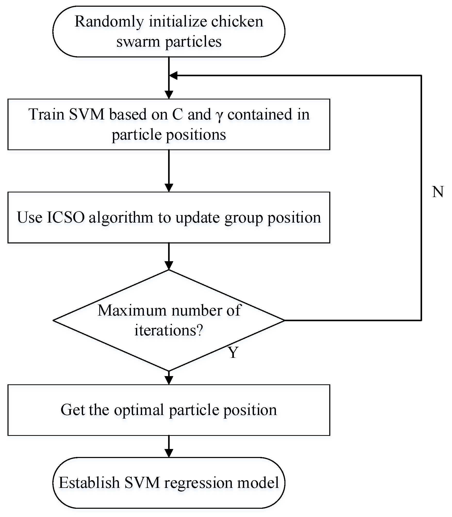
3.1. Support Vector Machine Prediction Model Based on Improved Chicken Swarm Algorithm

In order to find the appropriate penalty factor $C$ and kernel function parameters $\gamma$, this paper uses the improved chicken swarm algorithm (Improved CSO, ICSO) to search for SVM parameters, and it builds the ICSO-SVM dam horizontal displacement prediction model. Then, the question turns into finding the minimum value of the objective function. The specific implementation steps of the ICSO-SVM algorithm are as follows:

Step 1: Randomly generates the initial chicken swarm particles, and the penalty factor $C$ and kernel function parameters $\gamma$ constitute the position of each chicken swarm particle;

Step 2: According to the $C$ and $\gamma$ value of each particle, the SVM learns the training set, and it uses the mean square error function as the target fitness function;

Step 3: This step uses the ICSO algorithm to update the particle position of each chicken group in the population. When the iterative process ends, it outputs the optimal particle position, namely $C$ and $\gamma$ values;

Step 4: The output $C$ and $\gamma$ were used to establish an SVM regression model.

The flow chart shows the process of how the ICSO algorithm optimizes SVM parameters in Figure 1.

3.2. Modeling of Nonlinear Systems

In order to verify the effectiveness of the improved chicken swarm algorithm to optimize the SVM model, a nonlinear system is used for simulation experiments, see Equation (1), and the nonlinear system has been used in several articles [23,24,25] to verify the prediction model performance.

$$y(t+1)=\frac{y(t)y(t-1)[y(t)+2.5]}{1+y^2(t)+y^2(t-1)}+u(t)$$

(1)

where $1\le t\le 1000$, $y(0)=0$, $y(1)=0$, $u(t)=\sin (2\pi t/25)$, and 800 samples (from $t=1$ to $t=800$) are selected for training, and samples (from $t=801$ to $t=1000$) are selected for testing; then, the model can be described by the following Equation (2):

$$y(t+1)=f(y(t),y(t-1),u(t))$$

(2)

It can be seen from Equation (2) that the ICSO-SVM model has three inputs $y(t)$, $y(t-1)$, $u(t)$, and an output $y(t+1)$. As shown in Figure 2 and Figure 3, the output $y(t+1)$ can be inferred based on the historical experience $y(t)$ and $y(t-1)$; however, future trends are not all evolved according to the historical experience, and they are also affected by external factors. $u(t)$ can be regarded as another important influencing factor of the actual output, and adding the $u(t)$ value to the input can reflect the actual situation more objectively.

In the simulation experiment, 800 training samples are used to train the ICSO-SVM model, and then, 200 unknown testing samples are used to input the trained model for prediction. The predicted value and prediction error are shown in Figure 4 and Figure 5, respectively.

It can be seen from Figure 4 that the nonlinear system model which is established by ICSO-SVM is effective, and the predicted curve can effectively follow the actual value curve. It can be seen from Figure 5 that the prediction error of the ICSO-SVM model floats in the interval between [−0.25, 0.25], indicating that the ICSO-SVM model has a high prediction accuracy.

3.3. Evaluation Indicators

In order to evaluate the advantages and disadvantages of the established model, the average mean absolute error (MAE), root mean square error (RMSE) and determination coefficient $R^2$ are used as evaluation indicators to analyze the prediction results. The formula is as follows:

$$MSE=\frac{1}{N}{\displaystyle \sum _{i=1}^N{\left(y_i-o_i\right)}^2}$$

(3)

$$RMSE=\sqrt{\frac{1}{N}{\displaystyle \sum _{i=1}^N{\left(y_i-o_i\right)}^2}}$$

(4)

$$R^2=1-\frac{{\displaystyle \sum _{i=1}^N{(y_i-o_i)}^2}}{{\displaystyle \sum _{i=1}^N{(y_i-{\overline{y}}_i)}^2}}$$

(5)

where $y_i$ and $o_i$ are the measured value and the measured average value, respectively; ${\overline{y}}_i$ is the predicted value; and N is the number of observation samples. Among them, the MAE and the RMSE reflect the error between the predicted value and the measured value, and the determination coefficient $R^2$ reflects the fitting degree of the model and the influencing factors.

4. Case Study

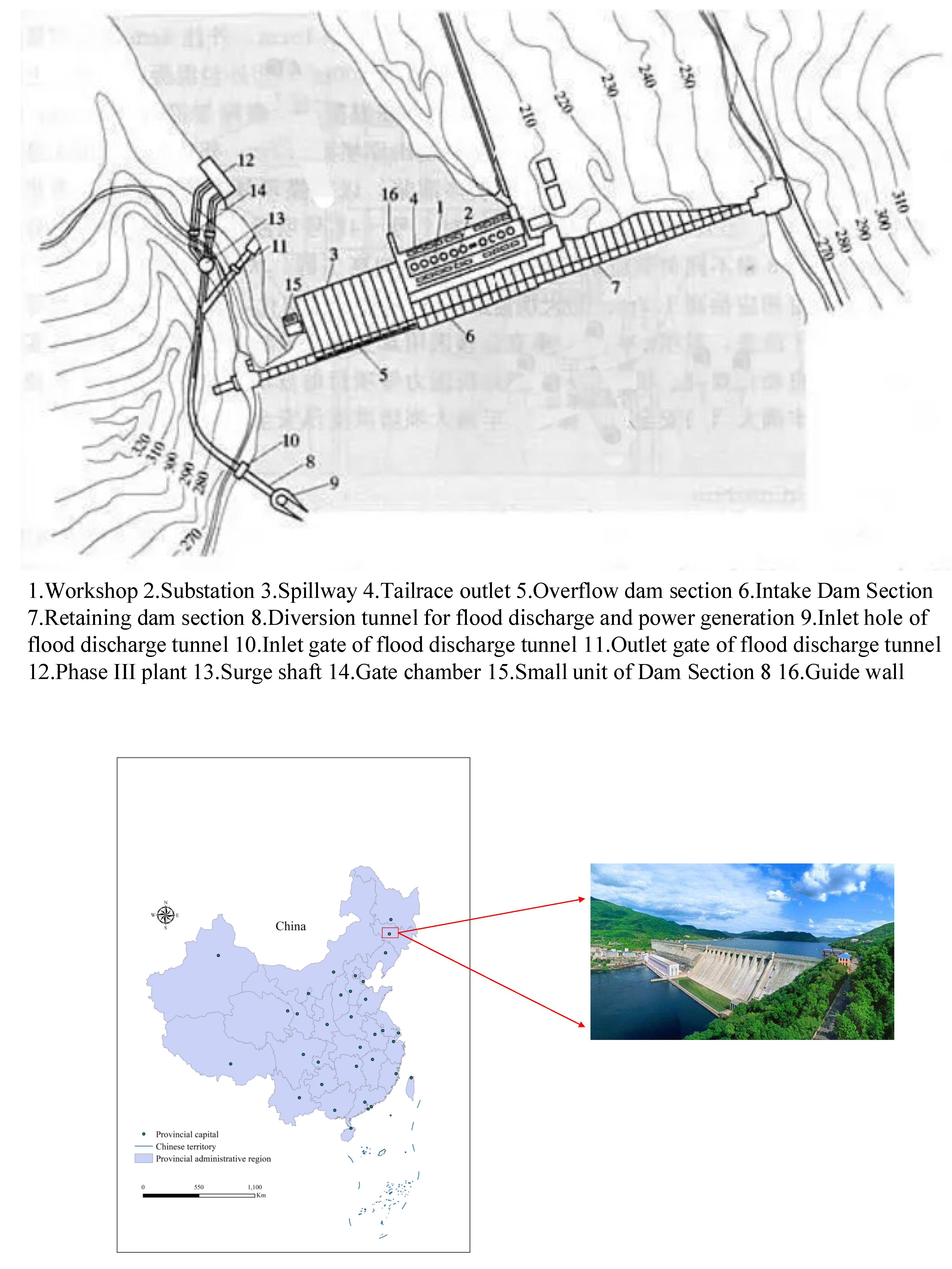
4.1. Engineering Experiment

Dams can be mainly divided into two types: concrete dams and earth-rock dams. At present, concrete dams are the mainstream, and among them, concrete gravity dams are the most common. Similar to FengMan Dam, a lot of dam hydraulic engineering utilizes concrete gravity. The monitoring data in this paper come from the FengMan Dam in Jilin Province. Since FengMan Dam is the earliest gravity dam built in China, it is representative and time-honored. Therefore, this paper selected its monitoring date for study. The FengMan Dam, a gravity dam built in 1937, is 80.5 m high, as shown in Figure 6. The total concrete volume of it is 1.94 million cubic meters. FengMan Dam is a cohesive soil homogeneous dam, and its underlying strata from bottom to top mainly are: triassic shale, which has no direct connection with the dam body; tertiary clay fine sand, with a permeability coefficient of 0.01 mm/s and thickness of 5–11 m; the quaternary sand and gravel layer, which is the main leakage channel of the dam and has a permeability coefficient of 0.1–0.3 mm/s and thickness of 5–22 m; the thickness of quaternary clay layer, which is 4–22 m and has the characteristic of low liquid limit and weak water permeability. The deformation observation of FengMan Dam began in the early 1970s, and the method of tension wire alignment was initially used. In order to know the operation status of the dam accurately, it is necessary to monitor the deformation of the dam. The monitoring contents mainly include changes in settlement, inclination, and cracks. The monitoring frequency is twice a year: one is in May before the flood season and another in November after the flood season. There is a 19# settlement monitoring point at 0 + 333 m of the dam, and its monitoring data are relatively complete. The monitoring results are shown in

Table 1. Monitoring data of horizontal displacement value.

Number of Observation Periods	Observation Date	Horizontal Displacement (mm)	Upstream Water Level H (m)	Temperature T (℃)
1	4/01/1985	−1.30	251.20	−15.40
2	11/01/1985	−1.86	250.27	−17.20
3	18/01/1985	−2.69	249.47	−12.60
4	28/01/1985	−3.01	248.68	−25.30
5	8/02/1985	−4.45	248.22	−3.50
6	15/02/1985	−3.97	247.75	−10.10
7	26/02/1985	−4.20	247.12	−12.80
8	6/03/1985	−4.17	246.65	−8.50
9	13/03/1985	−4.64	246.14	−6.50
10	22/03/1985	−4.69	245.84	0.20
…	…	…
196	17/06/1988	−1.83	252.66	15.6
197	22/06/1988	−2.34	252.68	24.30
198	2/07/1988	−3.54	252.52	20.50
199	8/07/1988	−3.32	252.52	22.70
200	13/07/1988	−3.91	252.81	25.90

.

Up to now, according to the incomplete statistics, instruments such as sliding micrometer, multi-point displacement gauges, bedrock displacement gauges, bolt stress gauges, biaxial rock stress gauges, etc. have been embedded in the dam. The installation of special monitoring instruments for cracks has also been completed, and a large number of the monitoring instruments have been connected to the automatic monitoring system, so that the continuity, timeliness, synchronization, and reliability of monitoring data have been greatly improved. The amount of data information has also increased significantly

For the dam, after the reservoir is impounded, the dam bears a very large water load, which will inevitably produce the horizontal and vertical displacement, which is an important indicator for evaluating the safety of the dam. For a concrete dam, there are many factors that affect its deformation, but there are mainly three parts: water pressure, temperature, and time [26,27,28]. The model can be described as:

$$\delta ={\delta }_H+{\delta }_T+{\delta }_{\theta }$$

(6)

where $\delta$ is the displacement value of a certain point of the dam; ${\delta }_H$, ${\delta }_T$, ${\delta }_{\theta }$ are the water pressure, temperature, and time components of the dam displacement, respectively.

Taking FengMan Dam as an example, the SVM optimized by the improved chicken swarm algorithm (ICSO) is used to model and forecast the horizontal displacement of the dam crest in real time. Dam horizontal displacement monitoring data and the monitoring data of water pressure, temperature and time for 200 periods from 4 January 1985 to 13 July 1988 were selected for analysis. Among them, the data of 1–160 periods are used as training samples, and the data of 161–200 periods are used as test samples. The values for the 200 periods of dam horizontal displacement and deformation are shown in Figure 7.

4.2. Causes of Deformation

During the operation of a dam, deformation often occurs. Once the deformation reaches a certain degree, it will affect the normal operation of the dam and even cause accidents. Therefore, during the process of dam construction and operation, the deformation observation shall be performed well to ensure its safety. During dam monitoring, the main causes of dam deformation were found, which are as follows:

(1)

Natural causes: One of the primary factors leading to the dam deformation is natural factors, especially under natural conditions such as complex soil physical properties, unclear engineering properties, and abnormal temperature fluctuations; dams are easily deformed [29]. For example, when the basic geological conditions of a dam are unstable, uneven subsidence may occur; when a dam is built on a soil foundation, the subsidence occurs due to the plastic deformation of the soil foundation; when the temperature and groundwater level in the area where the dam is located vary seasonally, regular changes in deformation will occur [30].

(2)

Causes of the dam itself: Another important factor leading to the dam deformation is the dam itself [31]. The structure design, its own weight, type, and the load of the dam are all directly related to the deformation. In addition, during the construction and operation process, because of the improper design, field survey, operation and management, it will also lead to some additional deformation of the dam. In this regard, in the overall design of the dam structure, the selection of the type frame, and the load and pressure experiments, it is necessary to combine the site, demonstrate scientifically, and follow the design requirements strictly [32]. Meanwhile, in the process of field survey, construction, management and maintenance, it is necessary to master the key points that may cause subsidence and strive to solve them by the most optimized method [33].

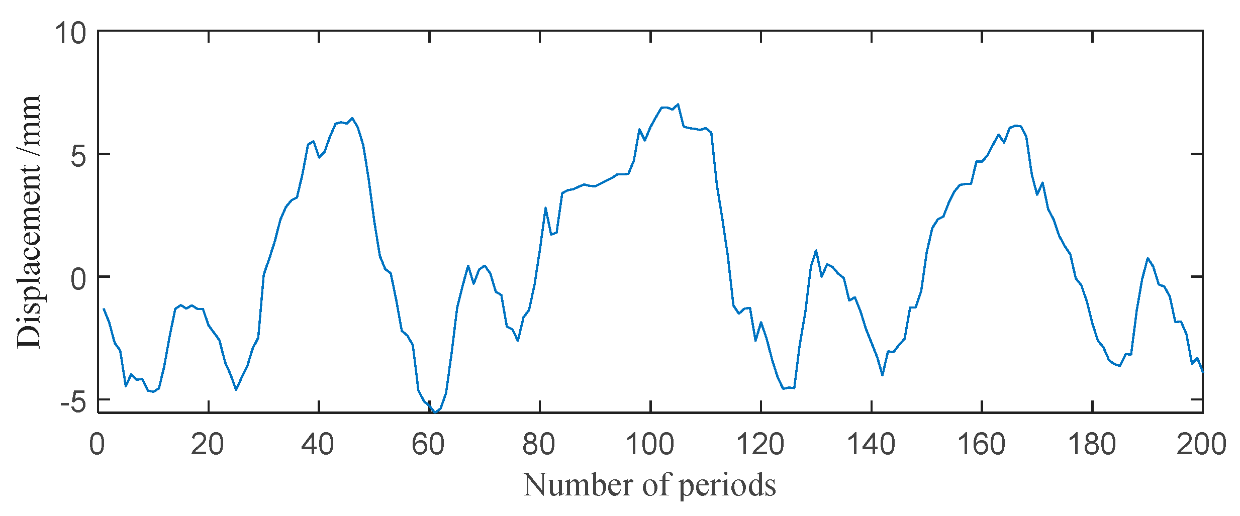
4.3. Data Preprocessing

The input of the ICSO-SVM model for dam deformation monitoring is determined by the number of factors that affect the amount of deformation observed. According to the introduction in Section 2, there are three types of factors that affect the horizontal displacement of concrete gravity dams: namely, water pressure, temperature and time. Among them, there are three water pressure factors $H$($H_1$, $H_1{}^2$, $H_1{}^3$). The temperature factor $T_0$ takes four sine and cosine harmonic factors ($\sin (2\mathsf{\pi }t/365)$, $\cos (2\mathsf{\pi }t/365)$, $\sin (4\mathsf{\pi }t/365)$, and $\cos (4\mathsf{\pi }t/365)$). The time factor takes two items $\theta$ and $\ln (\theta )$, where $\theta =0.01t$, $t$ is the cumulative number of days from the initial observation to the current observation. Reference [23] used the method of mean influence value (MIV) combined with BP neural network to deeply analyze the influence factors, considering that selecting $H_1$, $T_0$, $\sin (2\mathsf{\pi }t/365)$, $\sin (4\mathsf{\pi }t/365)$, $\theta$ and $\ln (\theta )$ can achieve a better prediction effect. Therefore, this paper selects these six influencing factors as the input of the model, and the output is the horizontal displacement value of the dam. The statistical results are shown in

Table 2. Input and output of prediction model.

Sample	Input						Output
	${\mathit{H}}_1/\mathbf{m}$	${\mathit{T}}_0$/°C	$\mathbf{sin}(2\mathsf{\pi }\mathit{t}/365)$	$\mathbf{sin}(4\mathsf{\pi }\mathit{t}/365)$	$\mathit{\theta }$	$\mathbf{ln}(\mathit{\theta })$	Horizontal Displacement Value/mm
1	251.200	−15.400	0	0	0	0	−1.300
2	250.270	−17.200	0.120	0.238	0.070	−2.659	−1.860
3	249.470	−12.600	0.239	0.464	0.140	−1.966	−2.690
4	248.680	−25.300	0.402	0.735	0.240	−1.427	−3.010
5	248.220	−3.500	0.567	0.934	0.350	−1.050	−4.450
6	247.750	−10.100	0.662	0.992	0.420	−0.868	−3.970
7	247.120	−12.800	0.791	0.968	0.530	−0.635	−4.200
8	246.650	−8.500	0.868	0.863	0.610	−0.494	−4.170
9	246.140	−6.500	0.921	0.718	0.680	−0.386	−4.640
10	245.840	0.200	0.970	0.471	0.770	−0.261	−4.690
…	…	…	…	…	…	…	…
…	…	…	…	…	…	…	…
199	252.520	22.700	−0.060	0.120	12.810	2.550	−3.320
200	258.810	25.900	−0.146	0.289	12.860	2.554	−3.910

.

There are large differences in the numerical magnitudes of the dimensions in the sample feature vector. If the model training is performed directly, the smaller dimension level data will be ignored, which cannot reflect its function, and it can even cause the model to fail to converge. After many simulation experiments, it is shown that the model is sensitive to the data between [−1, 1]. In order to resolve the difference between dimension levels, it is generally necessary to normalize the initial sample data. The normalized data have a positive effect on network learning, so after collecting the original data, this paper performs some preprocessing. There are many normalization methods [34,35,36]. In order to avoid the interference of extreme data on network training, this paper normalizes the experimental data to [−1, l] by Equation (7).

$$y=\frac{2(x-x_{\min })}{x_{\max }-x_{\min }}-1$$

(7)

where $y$ represents the normalized data; $x$ denotes the original data; $x_{\max }$ and $x_{\min }$ represent the maximum and minimum values in the original data, respectively.

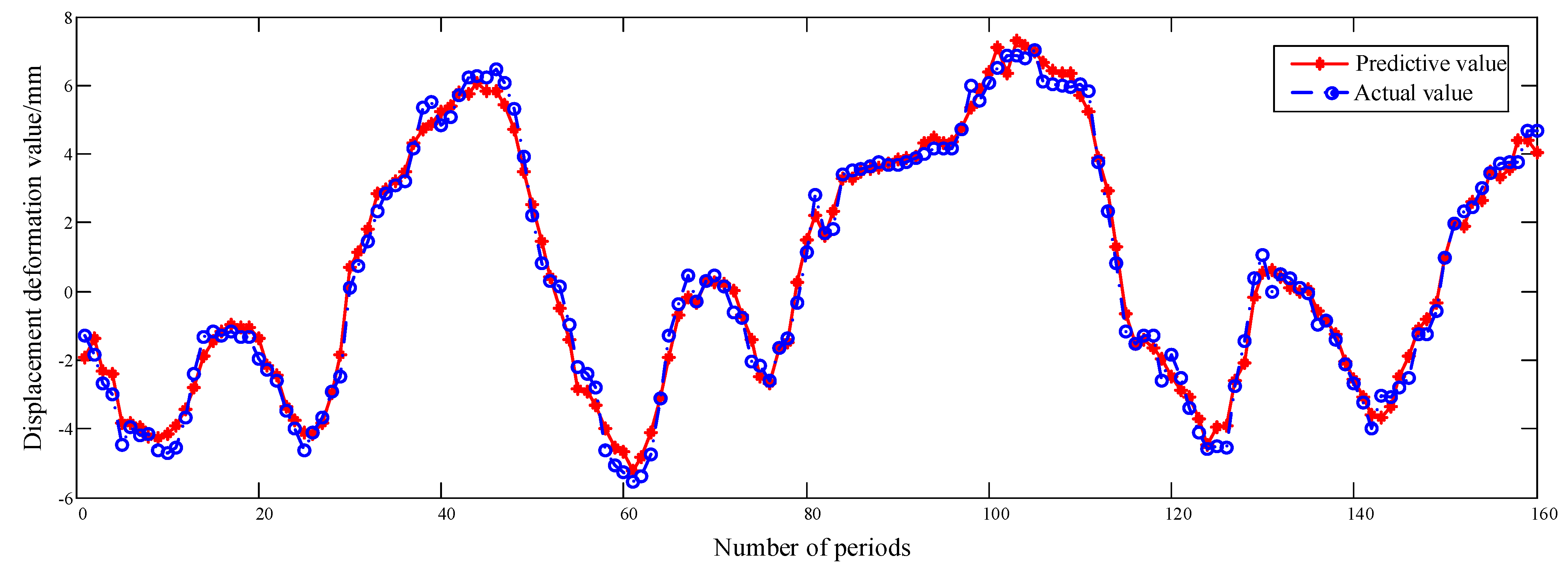
4.4. Dam Deformation Prediction

The basic chicken swarm algorithm and the improved chicken swarm algorithm are used to optimize the penalty factor and kernel function parameters of the SVM, and the mean square error is used as the fitness function to iterate. In the basic chicken swarm algorithm, the population size is 30, the maximum number of iterations is 200, the rooster size accounts for 15% of the total population, while the hens account for 70%. Among the individual hens, the hens with chicks account for 50%. The update interval is 10 generations. In the improved chicken swarm algorithm, the parameters are $a_0=0.3$, $a_1=0.7$, $a_2=1.0$ and $FL\in [0.4,1]$. After the first 50 iterations, the optimal fitness curves of the basic chicken swarm algorithm and the improved chicken swarm algorithm are shown in Figure 8.

It can be seen from Figure 8 that the optimal fitness value obtained by the improved chicken swarm algorithm at the initial stage is not ideal, but as the iteration progresses, the optimal fitness value drops rapidly and becomes lower than the basic chicken swarm algorithm. It shows that the improved chicken swarm algorithm adaptively adjusts the inertia weights as the environment around the population changes, thus balancing the local search and global search of the algorithm, and it finally searches for more superior SVM parameters with faster convergence. Finally, the optimal SVM parameters are obtained. Using SVM parameters, 180 training samples were learned, and an ICSO-SVM model was established for prediction. Among them, the fitting of the ICSO-SVM model to the training samples is shown in Figure 9.

It can be seen from Figure 10 that the fitting curve of the horizontal displacement of the dam for 180 periods follows the actual value curve well, indicating that the ICSO-SVM model has trained the dam training samples adequately, and it can be used for testing unknown samples.

4.5. Results Analysis and Comparison

The trained CSO-SVM and ICSO-SVM models are used to test 181–200 unknown samples, respectively. The prediction results for the last 20 periods of the horizontal displacement of the dam are shown in Figure 10. See

Table 3. Comparison of horizontal displacement prediction results between ICSO-SVM and CSO-SVM models.

Number of Periods	Measured Displacement Value/mm	ICSO-SVM		CSO-SVM
		Predictive Value/mm	Prediction Error/mm	Predictive Value/mm	Prediction Error/mm
161	4.930	5.344	0.414	5.128	0.198
162	5.370	5.616	0.246	5.281	−0.089
163	5.770	5.768	−0.002	5.187	−0.583
164	5.450	5.910	0.460	5.166	−0.284
165	6.050	6.151	0.101	5.147	−0.903
166	6.130	5.682	−0.448	4.751	−1.379
167	6.120	6.086	−0.034	4.833	−1.287
168	5.690	5.907	0.217	4.578	−1.112
169	4.150	5.580	1.430	4.385	0.235
170	3.330	5.065	1.735	4.270	0.940
171	3.820	4.470	0.650	3.643	−0.177
172	2.750	3.197	0.447	2.846	0.096
173	2.320	2.114	−0.206	1.742	−0.578
174	1.650	0.789	−0.861	0.578	−1.072
175	1.240	0.335	−0.905	0.166	−1.074
176	0.910	−0.246	−1.156	−0.311	−1.221
177	−0.080	−0.427	−0.347	−0.423	−0.343
178	−0.350	−0.684	−0.334	−0.639	−0.289
179	−1.020	−0.923	0.097	−0.838	0.182
180	−1.910	−1.353	0.557	−1.216	0.694
181	−2.610	−1.963	0.647	−1.770	0.840
182	−2.880	−2.192	0.688	−1.979	0.901
183	−3.400	−2.298	1.102	−2.075	1.325
184	−3.560	−2.877	0.683	−2.657	0.903
185	−3.640	−3.203	0.437	−2.941	0.699
186	−3.150	−2.537	0.613	−2.294	0.856
187	−3.180	−2.566	0.614	−2.288	0.892
188	−1.400	−1.282	0.118	−1.126	0.274
189	−0.100	−0.840	−0.740	−0.700	−0.600
190	0.750	0.069	−0.681	0.028	−0.722
191	0.400	−0.084	−0.484	−0.035	−0.435
192	−0.320	0.045	0.365	0.067	0.387
193	−0.400	0.098	0.498	0.107	0.507
194	−0.810	−0.076	0.734	−0.025	0.785
195	−1.860	−0.516	1.344	−0.348	1.512
196	−1.830	−0.791	1.039	−0.626	1.204
197	−2.340	−1.264	1.076	−0.994	1.346
198	−3.540	−1.644	1.896	−1.394	2.146
199	−3.320	−1.868	1.452	−1.599	1.721
200	−3.910	−1.944	1.966	−1.662	2.248

for the results of quantitative statistics in Figure 10.

In the genetic neural network, the population size is set to 30, the maximum number of iterations is set to 200, the training target is 0.01, the learning rate is 0.1, and the crossover probability is 0.9. After 200 generations of genetic calculation, the optimal fitness value optimization process is obtained, as shown in Figure 11.

As can be seen from Figure 10, the optimization curve of the optimal fitness value of GA presents a step-up shape, indicating that the algorithm is constantly searching for better initial parameters of the neural network.

The trained genetic neural network model was used to test 181–200 unknown samples, respectively. Figure 12 shows the predicted results of the dam horizontal displacement in the last 20 periods. See

Table 4. Comparison of horizontal displacement prediction results between the ICSO-SVM and GA-BP models.

Number of Periods	Measured Displacement Value/mm	ICSO-SVM		GA-BP
		Predictive Value/mm	Prediction Error/mm	Predictive Value/mm	Prediction Error/mm
161	4.930	5.344	0.414	4.979	0.049
162	5.370	5.616	0.246	5.362	−0.008
163	5.770	5.768	−0.002	5.921	0.151
164	5.450	5.910	0.460	6.111	0.661
165	6.050	6.151	0.101	6.316	0.266
166	6.130	5.682	−0.448	6.734	0.604
167	6.120	6.086	−0.034	6.693	0.573
168	5.690	5.907	0.217	6.309	0.619
169	4.150	5.580	1.430	5.865	1.715
170	3.330	5.065	1.735	5.608	2.278
171	3.820	4.470	0.650	4.444	0.624
172	2.750	3.197	0.447	3.401	0.651
173	2.320	2.114	−0.206	2.494	0.174
174	1.650	0.789	−0.861	1.332	−0.318
175	1.240	0.335	−0.905	1.584	0.344
176	0.910	−0.246	−1.156	1.467	0.557
177	−0.080	−0.427	−0.347	1.623	1.703
178	−0.350	−0.684	−0.334	1.280	1.630
179	−1.020	−0.923	0.097	0.857	1.877
180	−1.910	−1.353	0.557	−0.063	1.847
181	−2.610	−1.963	0.647	−1.306	1.304
182	−2.880	−2.192	0.688	−1.741	1.139
183	−3.400	−2.298	1.102	−2.022	1.378
184	−3.560	−2.877	0.683	−3.260	0.300
185	−3.640	−3.203	0.437	−4.027	−0.387
186	−3.150	−2.537	0.613	−3.712	−0.562
187	−3.180	−2.566	0.614	−3.561	−0.381
188	−1.400	−1.282	0.118	−2.253	−0.853
189	−0.100	−0.840	−0.740	−0.926	−0.826
190	0.750	0.069	−0.681	0.546	−0.204
191	0.400	−0.084	−0.484	0.325	−0.075
192	−0.320	0.045	0.365	0.479	0.799
193	−0.400	0.098	0.498	0.532	0.932
194	−0.810	−0.076	0.734	0.174	0.984
195	−1.860	−0.516	1.344	−0.647	1.213
196	−1.830	−0.791	1.039	−1.176	0.654
197	−2.340	−1.264	1.076	−1.802	0.538
198	−3.540	−1.644	1.896	−2.287	1.253
199	−3.320	−1.868	1.452	−2.352	0.968
200	−3.910	−1.944	1.966	−2.184	1.726

for the results of quantitative statistics in Figure 12.

In order to illustrate the superiority of the ICSO-SVM model for the prediction of the horizontal displacement of the dam, the CSO-SVM and the Genetic Neural Network (GA-BP) model were used for comparison. The three models (ICSO-SVM, CSO-SVM and GA-BP) first learn from 1–180 training samples, and then, they use the trained models to test 181–200 unknown samples, respectively. In order to visually compare the prediction results of the three models, Figure 13 presents a unified representation of the three models.

As can be seen from Figure 14, the prediction curve of the ICSO-SVM model follows the measured value curve best. Compared with the CSO-SVM model, the prediction accuracy of the ICSO-SVM model is significantly higher than that of the CSO-SVM model in the period 161–175, and then, the prediction accuracy of the two models is comparable in the period 176–200. Compared with the GA-BP model, the prediction of the GA-BP model is more volatile, while the prediction of the ICSO-SVM model is more stable. The prediction error curves of the three dam horizontal displacement prediction models are shown in Figure 14.

It can be seen from Figure 14 that the prediction error fluctuation range of the ICSO-SVM model is [−1.156, 1.966], and the length of the error fluctuation interval is 3.122 mm. The prediction error fluctuation range of the CSO-SVM model is [−1.379, 2.248], and the length of the error fluctuation interval is 3.627 mm. The prediction error fluctuation range of the GA-BP model is [−0.853, 2.278], and the length of the error fluctuation interval is 3.131 mm. Compared with the CSO-SVM and GA-BP models, the error fluctuation range of the ICSO-SVM model is the smallest, indicating that the prediction error of the ICSO-SVM model has a smaller fluctuation range around 0 mm.

The following is a quantitative analysis of the prediction accuracy. From Table 3, it can be found that the minimum absolute error predicted by the ICSO-SVM model is 0.002 mm in the 163rd period, and the maximum absolute error is 1.966 mm in the 200th period. The minimum absolute error predicted by the CSO-SVM model is 0.089 mm in the 162nd period, and the maximum absolute error is 2.248 mm in the 200th period, which indicates that the error fluctuation range predicted by the ICSO-SVM model is smaller than that of the CSO-SVM model. It can be found from

Table 5. Mean absolute error and root mean square error of different dam horizontal displacement prediction models.

Model	MAE/mm	RMSE/mm	${\mathit{R}}^2/\mathbf{mm}$
ICSO-SVM	0.696	0.854	0.9558
CSO-SVM	0.826	0.979	0.9556
GA-BP	0.828	1.010	0.9457

that the minimum absolute error predicted by the ICSO-SVM model is 0.002 mm in the 163rd period, and the maximum absolute error is 1.966 mm in the 200th period. The minimum absolute error predicted by the GA-BP model is 0.008 mm in the 162nd period, and the maximum absolute error is 2.278 mm in the 170th period, which indicates that the error fluctuation range predicted by the ICSO-SVM model is smaller than that of the GA-BP model. The MAE and the RMSE of the ICSO-SVM, CSO-SVM and GA-BP models are calculated based on the prediction of the dam horizontal displacement values in Table 3 and Table 4, as shown in Table 5.

It can be seen from Table 4 that the MAE of the ICSO-SVM model is 0.696 mm, which is smaller than 0.826 mm for the CSO-SVM model and 0.828 mm for the GA-BP model. The RMSE of the ICSO-SVM model is 0.854 mm, which is smaller than 0.979 mm for the CSO-SVM model and 1.010 mm for the GA-BP model. Among them, the values of the three model determination coefficients are 0.9558, 0.9556, and 0.9457, respectively. The determination coefficient represents the extent to which the variation of the independent variable accounts for the variation of the dependent variable. The larger the determination coefficient is, the higher the proportion of variation caused by independent variables in the dependent variables are, and the better the generalization performance of the model.

To sum up, it shows that the ICSO-SVM dam horizontal displacement prediction model is effective, and the prediction accuracy is better than the CSO-SVM and GA-BP dam horizontal displacement prediction models.

5. Discussion

The occurrence of safety problems in dams will cause very serious consequences, so it is necessary to monitor the dams’ deformation. The prediction and analysis based on the deformation monitoring data are important means to ensure the safe operation of dams. On the basis of sorting out and summarizing the previous research results, this paper also made some meaningful explorations and attempts in the field of dam deformation prediction, and it obtained some useful conclusions and achievements. However, due to time constraints, limited academic level and knowledge structure, there are still many issues that need further research, including the following aspects:

(1)

There are many methods for predicting dam deformation, mainly including a time series model, regression analysis model, neural network model, gray prediction model, Kalman filter, etc. All of these models can predict the dam deformation, but the accuracy of them is different. Some models have high accuracy, and the prediction effect can meet the needs, while others have low accuracy, and the prediction effect is not satisfactory. Therefore, many scholars began to combine a single model into a combined model. By choosing suitable sub-models and combining methods, the advantages of each model can be exploited to effectively improve the prediction accuracy. However, if the sub-model or combination method is selected improperly, instead of improving the prediction accuracy, it rather affects the prediction effect, which requires scholars to conduct sufficient and reliable research on their prediction models.

(2)

This paper studies the prediction model, which is verified by an example through the horizontal displacement monitoring data of the dam. However, the dam safety monitoring model is not only the monitoring and forecasting of the horizontal displacement but also the vertical displacement and land subsidence. It is of great engineering application value to carry out modeling prediction and comprehensively evaluate the safe operation status of dams.

(3)

With the development of surveying and mapping science and technology, the methods and means of dam deformation monitoring are becoming more and more advanced. The degree of automatic dam deformation monitoring becomes higher, and research, analysis and prediction of real-time dynamic monitoring data is a hot field today.

(4)

Dam deformation monitoring is a multi-disciplinary and multi-field work. Experts and scholars need to continue to improve it by introducing the latest research results of other emerging disciplines.

6. Conclusions

Dams have the functions of flood control, drought resistance, power generation, shipping, irrigation, aquaculture, tourism, etc. They play a vital role in our country’s national economic construction. However, once a safety problem occurs in the dam, it will bring huge loss of life and properties to the surrounding people. Dams deformation monitoring is necessary, and the prediction and analysis based on the deformation monitoring data are important means to ensure the safety of the dam. Dam deformation is affected by various factors such as water pressure, temperature, and geological conditions, and it is also limited by management costs and levels. Therefore, using historical dam deformation monitoring data to predict is an economical and effective method. Since the dam deformation monitoring data have the characteristics of nonlinearity, trending, periodicity and randomness, a combined model ICSO-SVM is constructed in this paper. At the same time, the experiment was carried out using 200 sets of dam horizontal displacement data measured from 4 January 1985 to 13 July 1988 at the FengMan Dam. After preprocessing the data, the prediction results of the combined model ICSO-SVM, classical combination models CSO-SVM model and GA-BP model are compared and analyzed. The main research contents and conclusions of the paper are as follows:

(1)

The CSO algorithm has been improved. Since the CSO algorithm easily falls into the local optimum and the convergence speed is slow in the evolution process, this paper integrates the inertia weight, which is determined by the foraging speed, and the aggregation degree into the optimization process of the CSO algorithm to increase the optimization time of the CSO regarding the population diversity and improve the ability of individual chickens to break through the local optimum. The simulation experiment is carried out through the test function, and the experimental results show that the optimization accuracy of the ICSO algorithm is better than that of the basic CSO algorithm, and the prediction accuracy has been improved several times.

(2)

A dam deformation prediction model based on the ICSO algorithm to optimize SVM is established. Compared with the traditional CSO algorithm, the ICSO algorithm optimizes the SVM model with a higher prediction accuracy and stronger model generalization ability. The ICSO algorithm performs better than the CSO algorithm in the parameters optimization process, and the model prediction accuracy has been further improved. The dam deformation prediction model based on the ICSO algorithm optimizing SVM has good prediction ability of dam deformation. By selecting the appropriate network structure and assigning the optimal parameters obtained by the ICSO algorithm to the SVM network, the dam deformation prediction value with high accuracy can be calculated.

(3)

The model is applied to an engineering example. Through the prediction and analysis of settlement data of the FengMan Dam monitoring point, the deformation prediction results for FengMan Dam by the combined model ICSO-SVM as well as other combined models CSO-SVM and GA-BP are compared and analyzed. The prediction accuracy of each model is ranked as ICSO-SVM model, CSO-SVM model and GA-BP model sequentially. The RMSE and MAE values of the ICSO-SVM model with the best prediction performance are the minimum values, while $R^2$ exceeds 0.9, and the prediction accuracy can meet the actual needs of the project.

References

1. Salazar, F.; Morán, R.; Toledo, M.Á.; Oñate, E. Data-based models for the prediction of dam behaviour: A review and some methodological considerations. Arch. Comput. Methods Eng. 2017, 24, 1–21. [Google Scholar] [CrossRef]
2. Pisaniello, J.D.; Dam, T.T.; Tingey-Holyoak, J.L. International small dam safety assurance policy benchmarks to avoid dam failure flood disasters in developing countries. J. Hydrol. 2015, 531, 1141–1153. [Google Scholar] [CrossRef]
3. Ge, W.; Sun, H.; Zhang, H.; Li, Z.; Guo, X.; Wang, X.; Qin, Y.; Gao, W.; van Gelder, P. Economic risk criteria for dams considering the relative level of economy and industrial economic contribution. Sci. Total Environ. 2020, 725, 138139. [Google Scholar] [CrossRef] [PubMed]
4. Stefaniak, K.; Wróżyńska, M. On possibilities of using global monitoring in effective prevention of tailings storage facilities failures. Environ. Sci. Pollut. Res. 2018, 25, 5280–5297. [Google Scholar] [CrossRef]
5. Kaloop, M.R.; Elbeltagi, E.; Hu, J.W.; Elrefai, A. Recent advances of structures monitoring and evaluation using GPS-time series monitoring systems: A review. ISPRS Int. J. Geo-Inf. 2017, 6, 382. [Google Scholar] [CrossRef]
6. Liu, N.; Dai, W.; Santerre, R.; Kuang, C. A MATLAB-based Kriged Kalman Filter software for interpolating missing data in GNSS coordinate time series. GPS Solut. 2018, 22, 25. [Google Scholar] [CrossRef]
7. Yu, X.; Dan, D. Online frequency and amplitude tracking in structural vibrations under environment using APES spectrum postprocessing and Kalman filtering. Eng. Struct. 2022, 259, 114175. [Google Scholar] [CrossRef]
8. Li, G.; Dai, W.; Yang, G.; Liu, B. Application of Space-Time Auto-Regressive Model in Dam Deformation Analysis. Geomat. Inf. Sci. Wuhan Univ. 2015, 40, 877–881. (In Chinese) [Google Scholar]
9. Oro, S.R.; Mafioleti, T.R.; Neto, A.C.; Garcia, S.R.P.; Júnior, C.N. Study of the influence of temperature and water level of the reservoir about the displacement of a concrete dam. Int. J. Appl. Mech. Eng. 2016, 21, 107–120. [Google Scholar] [CrossRef]
10. Qin, X.Y.; Liu, L.L.; Chen, J.; Chen, F.D.; Huang, L.K.; Xie, S.F. Dam deformation forecast based on EMD-PSO-BP neural network model. J. Guilin Univ. Technol. 2017, 4, 641–646. (In Chinese) [Google Scholar]
11. Zhang, L.; Zhikuan, X.U.; Luo, Y.; Cheng, P. Dam deformation prediction based on evolutionary multiple kernels relevance vector machine. Sci. Surv. Mapp. 2017, 42, 188–192. (In Chinese) [Google Scholar]
12. Su, H.Z.; Li, X.; Yang, B.B.; Wen, Z. Wavelet support vector machine-based prediction model of dam deformation. Mech. Syst. Signal Process. 2018, 110, 412–427. [Google Scholar] [CrossRef]
13. Zhang, X.; Kano, M.; Tani, M.; Mori, J.; Ise, J.; Harada, K. Prediction and causal analysis of defects in steel products: Handling nonnegative and highly overdispersed count data. Control. Eng. Pract. 2020, 95, 104258. [Google Scholar] [CrossRef]
14. Guo, Y.; Hu, S.; Wu, W.; Wang, Y.; Senthilnath, J. Multitemporal time series analysis using machine learning models for ground deformation in the Erhai region, China. Environ. Monit. Assess. 2020, 192, 464. [Google Scholar] [CrossRef] [PubMed]
15. Bian, K.; Wu, Z. Data-based model with EMD and a new model selection criterion for dam health monitoring. Eng. Struct. 2022, 260, 114171. [Google Scholar] [CrossRef]
16. Li, M.; Pan, J.; Liu, Y.; Liu, H.; Wang, J.; Zhao, Z. A Deformation Prediction Model of High Arch Dams in the Initial Operation Period Based on PSR-SVM-IGWO. Math. Probl. Eng. 2021, 2021, 8487997. [Google Scholar] [CrossRef]
17. Meng, X.; Liu, Y.; Gao, X.; Zhang, H. A New Bio-Inspired Algorithm: Chicken Swarm Optimization. In Proceedings of the International Conference in Swarm Intelligence, Beijing, China, 25–28 June 2014; Springer: Cham, Switzerland, 2014; pp. 86–94. [Google Scholar]
18. Song, Y.; Wang, F.; Chen, X. An improved genetic algorithm for numerical function optimization. Appl. Intell. 2019, 49, 1880–1902. [Google Scholar] [CrossRef]
19. Katoch, S.; Chauhan, S.S.; Kumar, V. A review on genetic algorithm: Past, present, and future. Multimed. Tools Appl. 2021, 80, 8091–8126. [Google Scholar] [CrossRef]
20. Ding, Y.; Fu, X. Kernel-based fuzzy c-means clustering algorithm based on genetic algorithm. Neurocomputing 2016, 188, 233–238. [Google Scholar] [CrossRef]
21. Liang, H.; Wei, Q.; Lu, D.; Li, Z. Application of GA-BP neural network algorithm in killing well control system. Neural Comput. Appl. 2021, 33, 949–960. [Google Scholar] [CrossRef]
22. Wang, H.; Li, J.; Liu, L. Process optimization and weld forming control based on GA-BP algorithm for riveting-welding hybrid bonding between magnesium and CFRP. J. Manuf. Processes 2021, 70, 97–107. [Google Scholar] [CrossRef]
23. Sayed, G.I.; Tharwat, A.; Hassanien, A.E. Chaotic dragonfly algorithm: An improved metaheuristic algorithm for feature selection. Appl. Intell. 2019, 49, 188–205. [Google Scholar] [CrossRef]
24. Wen, L.; Cao, Y. Influencing factors analysis and forecasting of residential energy-related CO2 emissions utilizing optimized support vector machine. J. Clean. Prod. 2020, 250, 119492. [Google Scholar] [CrossRef]
25. Bharanidharan, N.; Rajaguru, H. Improved chicken swarm optimization to classify dementia MRI images using a novel controlled randomness optimization algorithm. Int. J. Imaging Syst. Technol. 2020, 30, 605–620. [Google Scholar] [CrossRef]
26. Dai, B.; Gu, C.; Zhao, E.; Qin, X. Statistical model optimized random forest regression model for concrete dam deformation monitoring. Struct. Control. Health Monit. 2018, 25, e2170. [Google Scholar] [CrossRef]
27. Wei, B.; Chen, L.; Li, H.; Yuan, D.; Wang, G. Optimized prediction model for concrete dam displacement based on signal residual amendment. Appl. Math. Model. 2020, 78, 20–36. [Google Scholar] [CrossRef]
28. Zhang, J.; Cao, X.; Xie, J.; Kou, P. An improved long short-term memory model for dam displacement prediction. Math. Probl. Eng. 2019, 2019, 6792189. [Google Scholar] [CrossRef]
29. Xiao, R.; Jiang, M.; Li, Z.; He, X. New insights into the 2020 Sardoba dam failure in Uzbekistan from Earth observation. Int. J. Appl. Earth Obs. Geoinf. 2022, 107, 102705. [Google Scholar] [CrossRef]
30. Du, Z.; Ge, L.; Ng, A.H.M.; Zhu, Q.; Horgan, F.G.; Zhang, Q. Risk assessment for tailings dams in Brumadinho of Brazil using InSAR time series approach. Sci. Total Environ. 2020, 717, 137125. [Google Scholar] [CrossRef]
31. Mata, J. Interpretation of concrete dam behaviour with artificial neural network and multiple linear regression models. Eng. Struct. 2011, 33, 903–910. [Google Scholar] [CrossRef]
32. Liu, C.; Ahn, C.R.; An, X.; Lee, S. Life-cycle assessment of concrete dam construction: Comparison of environmental impact of rock-filled and conventional concrete. J. Constr. Eng. Manag. 2013, 139, A4013009. [Google Scholar] [CrossRef]
33. Xia, J.; Zhang, Y.Y.; Xiong, L.H.; He, S.; Wang, L.F.; Yu, Z.B. Opportunities and challenges of the Sponge City construction related to urban water issues in China. Sci. China Earth Sci. 2017, 60, 652–658. [Google Scholar] [CrossRef]
34. Liguori, A.; Markovic, R.; Dam, T.T.H.; Frisch, J.; van Treeck, C.; Causone, F. Indoor environment data time-series reconstruction using autoencoder neural networks. Build. Environ. 2021, 191, 107623. [Google Scholar] [CrossRef]
35. Sovacool, B.K.; Kryman, M.; Laine, E. Profiling technological failure and disaster in the energy sector: A comparative analysis of historical energy accidents. Energy 2015, 90, 2016–2027. [Google Scholar] [CrossRef]
36. Liang, T.; Wang, S.; Lu, C.; Jiang, N.; Long, W.; Zhang, M.; Zhang, R. Environmental impact evaluation of an iron and steel plant in China: Normalized data and direct/indirect contribution. J. Clean. Prod. 2020, 264, 121697. [Google Scholar] [CrossRef]
Figure 1. Flow chart of ICSO algorithm optimizing SVM parameters.
Processes 10 01842 g001
Figure 2. Input curve of ISCO-SVM model of nonlinear system.
Processes 10 01842 g002
Figure 3. Output curve of ICSO-SVM model of nonlinear system.
Processes 10 01842 g003
Figure 4. Prediction curve of ICSO-SVM model of nonlinear system.
Processes 10 01842 g004
Figure 5. Prediction error of ICSO-SVM model of nonlinear system.
Processes 10 01842 g005
Figure 6. Geographic location map of FengMan Dam.
Processes 10 01842 g006
Figure 7. Horizontal displacement sequence of dam.
Processes 10 01842 g007
Figure 8. Optimization curve of dam model parameters.
Processes 10 01842 g008
Figure 9. Horizontal displacement fitting of dam training samples.
Processes 10 01842 g009
Figure 10. Prediction curve of optimized support vector machine model.
Processes 10 01842 g010
Figure 11. Optimization process of GA optimal fitness value.
Processes 10 01842 g011
Figure 12. Prediction curve of genetic neural network model.
Processes 10 01842 g012
Figure 13. Horizontal displacement prediction curves of three model dam test samples.
Processes 10 01842 g013
Figure 14. Prediction error curve of horizontal displacement of dam test samples.
Processes 10 01842 g014