Optimal Planning of Hybrid Electricity–Hydrogen Energy Storage System Considering Demand Response

Abstract

In recent years, the stability of the distribution network has declined due to the large proportion of the uses of distributed generation (DG) with the continuous development of renewable energy power generation technology. Meanwhile, the traditional distribution network operation mode cannot keep the balance of the source and load. The operation mode of the active distribution network (ADN) can effectively reduce the decline in operation stability caused by the high proportion of DG. Therefore, this work proposes a bi-layer model for the planning of the electricity–hydrogen hybrid energy storage system (ESS) considering demand response (DR) for ADN. The upper layer takes the minimum load fluctuation, maximum user purchase cost satisfaction, and user comfort as the goals. Based on the electricity price elasticity matrix model, the optimal electricity price formulation strategy is obtained for the lower ESS planning. In the lower layer, the optimal ESS planning scheme is obtained with the minimum life cycle cost (LCC) of ESS, the voltage fluctuation of ADN, and the load fluctuation as the objectives. Finally, the MOPSO algorithm is used to test the model, and the correctness of the proposed method is verified by the extended IEEE-33 node test system. The simulation results show that the fluctuation in the voltage and load is reduced by 62.13% and 37.06%, respectively.

1. Introduction

Distributed generation (DG) based on wind power and photovoltaic power generation can ensure the normal supply of electricity consumption while reducing the impact on the environment [1,2]. However, the high proportion of DG will have a serious impact on the operation stability of the distribution network [3,4]. An energy storage system (ESS) is an important distributed resource. Additionally, the demand response (DR) load is a demand-side energy management application in the distribution system. In the operation mechanism of DR, the formulation of the time-of-use strategy is extremely important. This can shift the peak load to the valley, thereby reducing the pressure on ADN during peak hours. It should be noted that the total load in a day does not change, and the obvious degree of the phenomenon of electricity load shifting is mainly affected by user behaviour, and not all users will respond to this regulation strategy. The rational allocation of ESS while considering DR can effectively reduce the impact of the high proportion of DG access and improve the operation stability of the actively distributed network (ADN). However, distribution network planning needs to consider the future load growth and power grid development needs, integrated users, and different interest groups’ win–win complex issues. The traditional distribution network cannot process the access of a high proportion of DG. ADN uses an active management model that integrates DG, ESS, and the user load. This management mode can effectively improve the safety and stability of the distribution network operation and economy, and give full play to the active use of DG [5,6,7].

At the same time, to reduce the impact of DG when it is accessing the ADN, it is necessary to configure the ESS in ADN to store the excess DG output in the energy storage medium so that the ESS can provide power when the load of ADN increases to ensure the normal operation of ADN. In addition, as an important part of ADN, the load changing is mainly caused by human subjective factors (for example, for residential electricity, the switching of electrical equipment, and for industrial electricity, the changing of factory output). These changes will cause the load pressure of ADN, which will reduce the operation stability of ADN. Therefore, it is necessary to call on residents’ load to reduce the use of high-power appliances during the peak period of electricity consumption and use them during the valley period of electricity consumption. The addition of the DR load can effectively achieve this goal [8,9,10]. On the electricity market, DR is mainly composed of two types: one is to sign an interruptible agreement with the user, which requires that it reduces or interrupts the electricity consumption during the peak load period to obtain relevant compensation. The scheme is mainly aimed at large industrial users because it has high power flexibility and is not suitable for small-scale distribution networks. The other is based on the price elasticity matrix, through the dynamic changes in electricity prices that affect the user’s electricity consumption behavior, as in the case of total electricity users which remain unchanged through the load shifting to achieve the ‘peak load shifting’ role, to reduce the net load fluctuations caused by DG.

Therefore, an effective configuration scheme is key to realizing the renewable energy consumption. At the same time, the rational use of the DR side load can maximize the benefits and reduce the load fluctuations caused by DG access. Reference [11] proposed a method to offset the uncertainty of the renewable energy output with the DR load. Taking the terminal load size and the balanced load strategy as the decision variables, a renewable energy consumption optimization model considering the renewable energy consumption target and economic target is established. Reference [12] proposed a multi-objective DR model based on user satisfaction, electricity expenditure satisfaction, and user satisfaction. However, it does not consider the stability index of the ADN, and it weights the multi-objective into a single objective by setting the weight method which lacks objectivity. Based on the integrated energy system considering the electric, thermal, and gas loads on the DR side, the authors in [13,14] used the Cplex solver to obtain the minimum operation and maintenance cost of the integrated energy system under the constraints. In [15], an optimal dispatch model with ESS was constructed based on the dynamic electricity price model, which reduced the cost of operation.

In recent years, ESS has become a key facility to promote the large-scale application of renewable energy and improve the resilience and economy of ADN due to its ability to adjust the power of the distribution network and transfer energy across time scales. The configuration of ESS on the distribution side plays an important role in improving the consumption rate of renewable energy, stabilizing the fluctuation of DG and solving the uncoordinated development of the network. However, the role of ESS in regulating ADN and accelerating DG applications depends to a large extent on the proper planning of ESS. The disorderly access of ESS may lead to problems such as voltage over-limit, increased load fluctuation, and endangering the grid operation.

In many studies of configuring ESS, determining how the ESS may reasonably access ADN is an important issue. In [16], a single-layer model was established to describe the economic optimization problem of the ESS configuration, without considering the coupling relationship between ESS and ADN. Aiming at reducing the ESS operation and maintenance cost and improving the voltage fluctuation and load fluctuation, reference [17] used the multi-objective mayfly algorithm (MOMA) to formulate the optimal location and capacity. In the optimal configuration of ESS with DR, it is necessary to consider the multiple indicators of the user side and the distribution side. If these indicators are optimized in the model at the same level, the local optimal phenomenon will be caused by the contradictory relationship between different objectives. Therefore, a bi-level optimization model is needed to solve this problem. In reference [18], a two-layer model and multiple indicators were established to optimize the configuration of a battery energy storage system (BESS). However, ADN planning needs to consider the long-term load growth, electromagnetic energy storage system charging, and discharging time scale as shorter, which is suitable for the short-term storage of electricity. As the most promising energy source in the 21st century, hydrogen is an energy storage medium with incomparable advantages over other energy storage media. For example, in combustible materials, compared to natural gas, hydrogen combustion products are only completely pollution-free water. In terms of storage stability, with the development of hydrogen storage technology in recent years, it has been possible to ensure the long-term safe storage and transportation of hydrogen. Moreover, in the medium and long-term, a hydrogen energy storage system (HESS) is more suitable for solving the problem of the coordinated matching of renewable energy and load in the regional power grid, accelerating energy transformation, and playing an important role in environmental protection [19,20,21]. In reference [22], an ESS planning model considering the mixed storage differentiation characteristics is established, and the genetic algorithm based on an elitist preservation strategy is used to optimize the configuration of the hybrid ESS. Reference [23] used a bi-layer model to optimize the configuration of the hybrid ESS. The upper-level objective function is the annual comprehensive cost of configuring ESS, and the lower-level objective function is the rate of wind and light abandonment. It does not consider DR. This configuration method requires a highly stable ADN and it is difficult to guarantee the satisfaction of users.

Considering DR while configuring ESS serves to further reduce the impact on ADN. Therefore, a bi-level programming model considering the DR side load and electricity–hydrogen hybrid ESS is established in this work. The bi-layer model can better coordinate various problems in ESS. The upper-level layer aims at the minimum net load fluctuation, user satisfaction with electricity, and user satisfaction with money, and affects the user’s electricity consumption behavior through the adjustment of a dynamic electricity price. The lower-level layer is concerned with the minimum life cycle cost (LCC), minimum net load fluctuation, and minimum voltage fluctuation of the electricity–hydrogen hybrid energy storage to improve the stability of the ADN while ensuring the economic benefits of investors. Finally, the feasibility of the model is verified by multi-objective particle swarm (MOPSO) in the extended IEEE-33 test node combined with the historical wind and light load data of a certain place. Meanwhile, a multi-objective artificial bee colony (MOABC) and multi-objective differential evolution (MODE) have been used as the comparison algorithm to verify the accuracy of MOPSO.

The main contribution of this work is:

(1) The demand side response model is established. The model describes the electricity consumption and purchase behavior of users under different electricity prices through the time-of-use electricity price strategy.

(2) A bi-layer optimization model is proposed. The model takes into account the economy and comfort of users’ electricity consumption, the economy of ESS and the change in the ADN operating index under the time-of-use strategy.

(3) The simulation test based on the IEEE-33 node test system is designed, and the MOPSO algorithm is used to solve the model. The simulation results show that the proposed model and solution method can obtain the optimal configuration scheme.

2. Demand Response Model

2.1. Time-Of-Use Price Model

After the implementation of this measure, the original electricity price in each period becomes:

$$p_{\mathrm{p}}=p_0·\left(1+\alpha \right),\cdots t\in T_{\mathrm{p}}$$

(1)

$$p_{\mathrm{u}}=p_0·\left(1+\beta \right),\cdots t\in T_{\mathrm{u}}$$

(2)

$$p_{\mathrm{v}}=p_0·\left(1+\gamma \right),\cdots t\in T_{\mathrm{v}}$$

(3)

where $p_{\mathrm{p}}$, $p_{\mathrm{u}}$, $p_{\mathrm{v}}$ represent the peak time, flat time, and valley time price after the implementation of the time-of-use price strategy, respectively; $p_0$ represents the electricity price set by the power supply company before the implementation of time-of-use price strategy; $\alpha$, $\beta$, $\gamma$ represent the price fluctuation range for three periods, respectively.

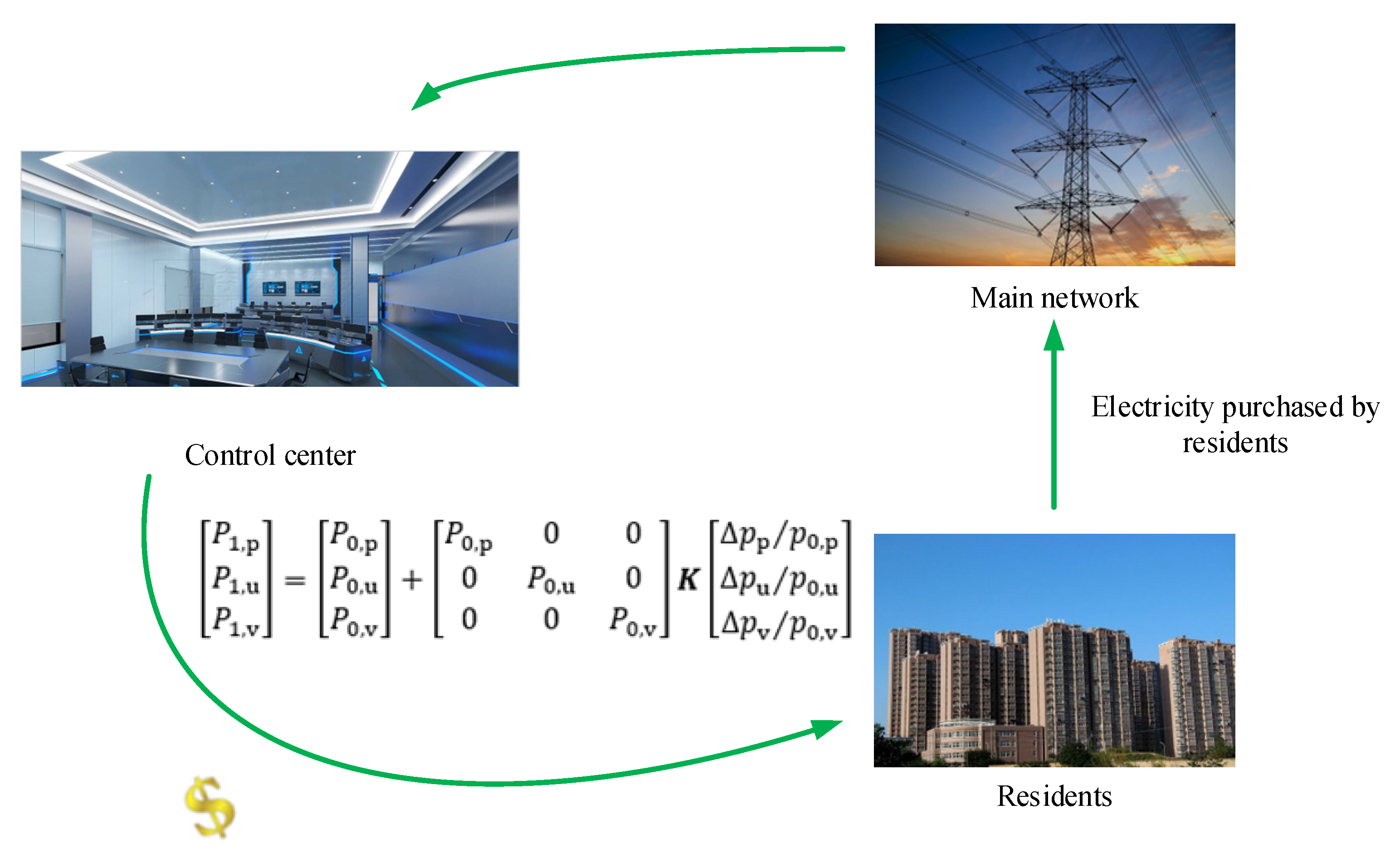
2.2. Electricity Price Elasticity Matrix Model

The electricity price elasticity matrix reflects the user changing their electricity consumption behavior according to different periods of time-of-use price. The relationship between the change in user electricity consumption and the change in electricity price is as follows:

$$k=\frac{\Delta L}{L}{\left(\frac{\Delta p}{p}\right)}^{-1}$$

(4)

where $\Delta L$ represents the load change value and $\Delta p$ represents the electricity price change value.

The peak, flat, and valley loads change as follows:

$$\left[\begin{array}{c}{P}_{1,\mathrm{p}}\\ P_{1,\mathrm{u}}\\ P_{1,\mathrm{v}}\end{array}\right]=\left[\begin{array}{c}{P}_{0,\mathrm{p}}\\ P_{0,\mathrm{u}}\\ P_{0,\mathrm{v}}\end{array}\right]+\left[\begin{array}{ccc}{P}_{0,\mathrm{p}}& 0& 0\\ 0& P_{0,\mathrm{u}}& 0\\ 0& 0& P_{0,\mathrm{v}}\end{array}\right]\mathit{K}\left[\begin{array}{c}\Delta p_{\mathrm{p}}/p_{0,\mathrm{p}}\\ \Delta p_{\mathrm{u}}/p_{0,\mathrm{u}}\\ \Delta p_{\mathrm{v}}/p_{0,\mathrm{v}}\end{array}\right]$$

(5)

where $P_{1,\mathrm{p}}$, $P_{1,\mathrm{u}}$, $P_{1,\mathrm{v}}$ represent the amount of electricity purchased by users from the superior power grid at three different times after the price changes, respectively; $p_{0,\mathrm{p}}$, $p_{0,\mathrm{u}}$, $p_{0,\mathrm{v}}$ represent the electricity prices of each period before the time-of-use price strategy is not implemented, respectively. $\mathit{K}$ is the price elasticity matrix, which is calculated as follows:

$$\mathit{K}=\left[\begin{array}{ccc}{k}_{\mathrm{pp}}& k_{\mathrm{pu}}& k_{\mathrm{pv}}\\ k_{\mathrm{up}}& k_{\mathrm{uu}}& k_{\mathrm{uv}}\\ k_{\mathrm{vp}}& k_{\mathrm{vu}}& k_{\mathrm{vv}}\end{array}\right]$$

(6)

This work uses the price elasticity matrix data described in reference [24] to describe the response of the load to electricity price changes. The active DR diagram is shown in Figure 1.

3. Energy Storage System Model

3.1. Battery Energy Storage System Model

In this work, BESS uses lithium batteries and lead-acid batteries as energy storage batteries, and its daily self-discharge rate is low (0.1~0.3%). Therefore, this work only considers the power exchange between BESS and ADN. The charge–discharge model of BESS is as follows:

$$\{\begin{array}{c}{E}_B\left(t+1\right)=E_B\left(t\right)+P_{\mathrm{charge},\mathrm{B}}\left(t\right)·\Delta t·{\alpha }_{\mathrm{charge},\mathrm{B}}\\ E_B\left(t+1\right)=E_B\left(t\right)+\left[P_{\mathrm{discharge},\mathrm{B}}\left(t\right)·\Delta t\right]/{\alpha }_{\mathrm{discharge},\mathrm{B}}\end{array}$$

(7)

where $P_{\mathrm{charge},\mathrm{B}}\left(t\right)$ represents the charging power of BESS at time $t$; $P_{\mathrm{discharge},\mathrm{B}}\left(t\right)$ represents the discharge power of BESS at time $t$; ${\alpha }_{\mathrm{charge},\mathrm{B}}$ and ${\alpha }_{\mathrm{discharge},\mathrm{B}}$ represent the charge–discharge efficiencies of BESS, respectively.

3.2. Hydrogen Energy Storage System Model

Electrolytic cell (EC), hydrogen storage tank (HT), and fuel cell (FC) are the main components of HESS. The EC can electrolyze water into hydrogen and oxygen in a short time, and its output power can be described as:

$$P_{\mathrm{EC}}=P_{\mathrm{charge},\mathrm{H}}·{\alpha }_{\mathrm{EC}}$$

(8)

where $P_{\mathrm{charge},\mathrm{H}}$ represents the charging power of HESS; ${\alpha }_{\mathrm{EC}}$ represents the conversion efficiency for EC.

The FC is the power output core of HESS, which supplies power to the ADN by consuming hydrogen in HT. The output power of HESS can be expressed by the output power of FC, as follows:

$$P_{\mathrm{discharge},\mathrm{H}}=Q_{\mathrm{HT}}·{\alpha }_{\mathrm{FC}}·q_{\mathrm{hydrogen}}$$

(9)

where $Q_{\mathrm{HT}}$ represents the hydrogen sent to FC from the HT; ${\alpha }_{\mathrm{FC}}$ represents the conversion efficiency for FC. $q_{\mathrm{hydrogen}}$ represent the calorific value constant of hydrogen, which is 39.3 kWh/kg.

4. Upper-Level Optimization Model

4.1. Upper-Level Objective Function

After considering DR, users will change their electricity consumption habits according to the time-of-use price. This behavior will reduce the load fluctuation and improve the stability of ADN. The formulation of time-of-use electricity prices will allow users to selectively adapt their electricity consumption at different times. The behavior of users to choose their electricity consumption period according to the electricity price will change the electricity comfort for the user.

After comprehensive consideration, this work selects the load fluctuation of ADN, users’ electricity purchase cost satisfaction, and the electricity comfort for user as the objective function in the upper optimization model.

4.1.1. The Load Fluctuation of ADN

$$\min F_1=\frac{{{\displaystyle \sum }}_{i=1}^{n_t}{{\displaystyle \sum }}_{t=1}^T\left|\sqrt{{[P_{1,i}\left(t\right)-P_{1,i}\left(t-1\right)]}^2}\right|}{n_t}$$

(10)

where $n_t$ represents the number of typical days; $P_{1,i}\left(t\right)$ and $P_{1,i}\left(t-1\right)$ represent the electricity purchased at time $t$ and time $\left(t-1\right)$ on typical days after the application of the time-of-use electricity price strategy, respectively. $T$ is 24 h.

4.1.2. User Purchase Cost Satisfaction

In this work, the ratio of user electricity expenditure before and after the real-time time-of-use electricity price is used as a measure of the user purchase cost satisfaction index, as follows:

$$\min F_2=\frac{{{\displaystyle \sum }}_{i=1}^{n_t}{{\displaystyle \sum }}_{t=1}^T\left(P_{1,i}\left(t\right)-p_{1,i}\left(t\right)\right)}{{{\displaystyle \sum }}_{i=1}^{n_t}{{\displaystyle \sum }}_{t=1}^T\left(P_{0,i}\left(t\right)-p_{0,i}\left(t\right)\right)}$$

(11)

where $P_{0,i}\left(t\right)$ and $p_{1,i}\left(t\right)$, respectively, represent the electricity price in the period $t$ before and after the application of the time-of-use electricity price on a typical day $i$;

4.1.3. Comfort of User

This work defines the comfort of a user through the ratio of the user’s transferred load to the initial load, which is specifically expressed as:

$$\min F_3=\frac{{{\displaystyle \sum }}_{i=1}^{n_t}{{\displaystyle \sum }}_{t=1}^T\left[P_{1,i}\left(t\right)-P_{0,i}\left(t\right)\right]}{{{\displaystyle \sum }}_{i=1}^{n_t}{{\displaystyle \sum }}_{t=1}^T{P}_{1,i}\left(t\right)}$$

(12)

4.2. Upper-Level Constraint

When the electricity price fluctuates greatly, it will have a great impact on the user’s electricity consumption habits and the stability of the power grid. Therefore, the usual price is equal to the price when time-of-use price is not considered. The peak price should be increased by 50% over the usual price, and the valley price should be reduced by 50% according to the usual price [25].

$$\{\begin{array}{c}{p}_{\mathrm{p},\left(\max ,\min \right)}=50\%·\pm p_{\mathrm{f}}\\ p_{\mathrm{u},\left(\max ,\min \right)}=\pm p_{\mathrm{f}}\\ p_{\mathrm{v},\left(\max ,\min \right)}=50\%·\pm p_{\mathrm{f}}\end{array}$$

(13)

where $p_{\mathrm{f}}$ represents the electricity price fluctuation in different periods ranging from 10% to 20%. This work takes 20%.

5. Lower-Level Optimization Model

5.1. Lower-Level Objective Function

5.1.1. The LCC of ESS

At present, most ESS cost models do not consider the impact of the type, technical characteristics, and life cycle of ESS in detail. The LCC model comprehensively considers all the costs of a life-cycle including the investment cost, maintenance cost, operation cost, and replacement cost, which can more comprehensively describe the economic cost of the whole life of ESS. Hence, this work takes the daily LCC of the hybrid ESS as the objective function as follows:

$$\min F_1=\frac{LC{C}_{\mathrm{BESS}}+LC{C}_{\mathrm{HESS}}}{365}$$

(14)

(1) The initial investment cost of BESS

$$c_{\mathrm{ICC},\mathrm{B}}={{\displaystyle \sum }}_{n=1}^{n_{\mathrm{BESS}}}\left(w_{\mathrm{B}}·P_{\mathrm{BESS}}+w_{\mathrm{I}}·E_{\mathrm{BESS}}\right)·{\gamma }_{\mathrm{B}}$$

(15)

$${\gamma }_{\mathrm{B}}=\frac{d}{{(1+d)}^{l_{\mathrm{B}}}-1}+d$$

(16)

where $n_{\mathrm{BESS}}$ represents the number of BESS installations; $E_{\mathrm{BESS}}$ represents the capacity of BESS; $P_{\mathrm{BESS}}$ represents the rated power rating of BESS; $w_{\mathrm{B}}$ represents the cost of battery; and $w_{\mathrm{I}}$ represents the cost of the inverter. ${\gamma }_{\mathrm{B}}$ represents the recovery coefficient of the equal annual value of BESS. $l_{\mathrm{B},\mathrm{H}}$ denotes the lifetime of BESS and HESS; $d$ denotes the discount rate [26].

(2) The maintenance cost of BESS

$$c_{\mathrm{MC},\mathrm{B}}={{\displaystyle \sum }}_{n=1}^{n_{\mathrm{BESS}}}\left({\mu }_{\mathrm{B}}·w_{\mathrm{B}}·P_{\mathrm{BESS}}+{\mu }_{\mathrm{I}}·w_{\mathrm{I}}·E_{\mathrm{BESS}}\right)·{\gamma }_{\mathrm{B}}$$

(17)

where ${\mu }_{\mathrm{B}}$ represents the proportion of the battery maintenance cost to investment cost; ${\mu }_{\mathrm{I}}$ represents the proportion of the inverter maintenance cost to investment cost.

(3) The operation cost of BESS

$$c_{\mathrm{OC},\mathrm{B}}=365{{\displaystyle \sum }}_{n=1}^{n_{\mathrm{BESS}}}{{\displaystyle \sum }}_{t=1}^T\left(c_{\mathrm{p}}\left(t\right)·P_{\mathrm{charge},\mathrm{B}}\left(t\right)+c_{\mathrm{s}}\left(t\right)·P_{\mathrm{discharge},\mathrm{B}}\left(t\right)\right)$$

(18)

where $c_{\mathrm{p}}\left(t\right)$ and $c_{\mathrm{s}}\left(t\right)$ are the purchase and sale prices of ESS, respectively.

(4) The replacement cost of BESS

$$c_{\mathrm{RC},\mathrm{BESS}}={{\displaystyle \sum }}_{n=1}^{n_{\mathrm{BESS}}}{{\displaystyle \sum }}_{r=1}^{r_{\mathrm{BESS}}}\frac{(1-{\delta }_{\mathrm{BESS}}{)}^{r_{\mathrm{time}}}}{{(1+d)}^{r_{\mathrm{time}}}}\left(w_{\mathrm{B}}·P_{\mathrm{BESS}}+w_{\mathrm{I}}·E_{\mathrm{BESS}}\right)·{\gamma }_{\mathrm{B}}$$

(19)

where $r_{\mathrm{BESS}}$ and $r_{\mathrm{time}}$ represent the battery replacement times and life cycle, respectively; ${\delta }_{\mathrm{BESS}}$ represents the annual decrease ratio of the BESS cost [27].

(5) The initial investment cost of HESS

$$c_{\mathrm{ICC},\mathrm{H}}={{\displaystyle \sum }}_{n=1}^{n_{\mathrm{HESS}}}\left(w_{\mathrm{FC}}·P_{\mathrm{FC}}+w_{\mathrm{EC}}·P_{\mathrm{EC}}+w_{\mathrm{HT}}·Q_{\mathrm{HT}}\right)·{\gamma }_{\mathrm{H}}$$

(20)

where $w_{\mathrm{FC}}$, $w_{\mathrm{EC}}$, and $w_{\mathrm{HT}}$denote the unit capacity cost of FC, EC, and HT, respectively; $P_{\mathrm{FC}}$, $P_{\mathrm{EC}}$ represent the rated power of FC and EC, respectively; $Q_{\mathrm{HT}}$ represents the capacity of HT. ${\gamma }_{\mathrm{H}}$ represents the recovery coefficient of the equal annual value of HESS.

(6) The maintenance cost of HESS

$$c_{\mathrm{MC},\mathrm{H}}={{\displaystyle \sum }}_{n=1}^{n_{\mathrm{HESS}}}\left((w_{\mathrm{FC}}·P_{\mathrm{FC}}+w_{\mathrm{EC}}·P_{\mathrm{EC}}\right)·{\mu }_{\mathrm{FC},\mathrm{EC}}+w_{\mathrm{HT}}·Q_{\mathrm{HT}}·{\mu }_{\mathrm{HT}})·{\gamma }_{\mathrm{B}}$$

(21)

where ${\mu }_{\mathrm{FC},\mathrm{EC}}$ represents the proportion of the FC and EC maintenance cost to investment cost; ${\mu }_{\mathrm{HT}}$ represents the proportion of HT maintenance cost to the investment cost.

(7) The operation cost of HESS

$$c_{\mathrm{OC},\mathrm{H}}=365{{\displaystyle \sum }}_{n=1}^{n_{\mathrm{HESS}}}{{\displaystyle \sum }}_{t=1}^T\left(c_{\mathrm{p}}\left(t\right)·P_{\mathrm{charge},\mathrm{H}}\left(t\right)+c_{\mathrm{s}}\left(t\right)·P_{\mathrm{discharge},\mathrm{H}}\left(t\right)\right)$$

(22)

(8) The replacement cost of HESS

The service life of FC and EC is 5–10 years, which is much shorter than that of HT (25 years). Therefore, the replacement cost of HESS only includes FC and EC.

$$c_{\mathrm{RC},\mathrm{HESS}}={{\displaystyle \sum }}_{n=1}^{n_{\mathrm{HESS}}}{{\displaystyle \sum }}_{r=1}^{r_{\mathrm{FC},\mathrm{EC}}}\frac{(1-{\delta }_{\mathrm{HESS}}{)}^{t_{\mathrm{FC},\mathrm{EC}}}}{{(1+d)}^{t_{\mathrm{FC},\mathrm{EC}}}}(w_{\mathrm{FC}}·P_{\mathrm{FC}}+w_{\mathrm{EC}}·P_{\mathrm{EC}})·{\gamma }_{\mathrm{H}}$$

(23)

where $r_{\mathrm{FC},\mathrm{EC}}$ represents the service life of FC and EC; $t_{\mathrm{FC},\mathrm{EC}}$ represents the replacement times of FC and EC, respectively.

5.1.2. The Load Fluctuation of ADN

$$\min F_2=\frac{\left[{{\displaystyle \sum }}_{i=1}^{n_t}{{\displaystyle \sum }}_{t=1}^T\sqrt{{\left(P_{2,i}\left(t\right)-P_{2,i}\left(t-1\right)\right)}^2}\right]}{n_t}$$

(24)

where $P_{2,i}\left(t\right)$ represents the power purchased from the upper power grid at time $t$ after the ESS is connected to the ADN.

5.1.3. The Voltage Fluctuation of ADN

$$\min F_3=\frac{\left[{{\displaystyle \sum }}_{i=1}^{n_t}{{\displaystyle \sum }}_{n=1}^{n_{\mathrm{nodes}}}\sqrt{{{\displaystyle \sum }}_{t=1}^T\frac{{\left(V_{n,i}\left(t\right)-{\overline{V}}_{n,i}\right)}^2}{T-1}}\right]}{n_t}$$

(25)

where $V_{n,i}\left(t\right)$ represents the voltage per unit value of node $n$ on a typical day at time $t$; ${\overline{V}}_{n,i}$ represents the average voltage of node $n$ on a typical day.

5.2. Constraints

Before and after the installation of ESS, the voltage of each node in the ADN needs to be satisfied within a certain safety range. At the same time, to ensure the rationality of the ESS configuration, the installation capacity and rated power of ESS also need to fall within a certain range. Moreover, the same type of ESS cannot be installed on the same node of the distribution network, and the node cannot be the contact point between the ADN and the upper power grid. These constraints can be described as:

$$V^{\min }\le V\le V^{\max }$$

(26)

$$\{\begin{array}{c}{E}_{\mathrm{ESS}}^{\min }\le E_{\mathrm{ESS}}\le E_{\mathrm{ESS}}^{\max }\\ P_{\mathrm{ESS}}^{\min }\le P_{\mathrm{ESS}}\le P_{\mathrm{ESS}}^{\max }\end{array}$$

(27)

$$\{\begin{array}{c}{L}_{\mathrm{ESS}}\ne L_{\mathrm{upper}}\\ L_{\mathrm{ESS},i}\ne L_{\mathrm{ESS},i+1}\end{array}$$

(28)

6. Solution of the Model

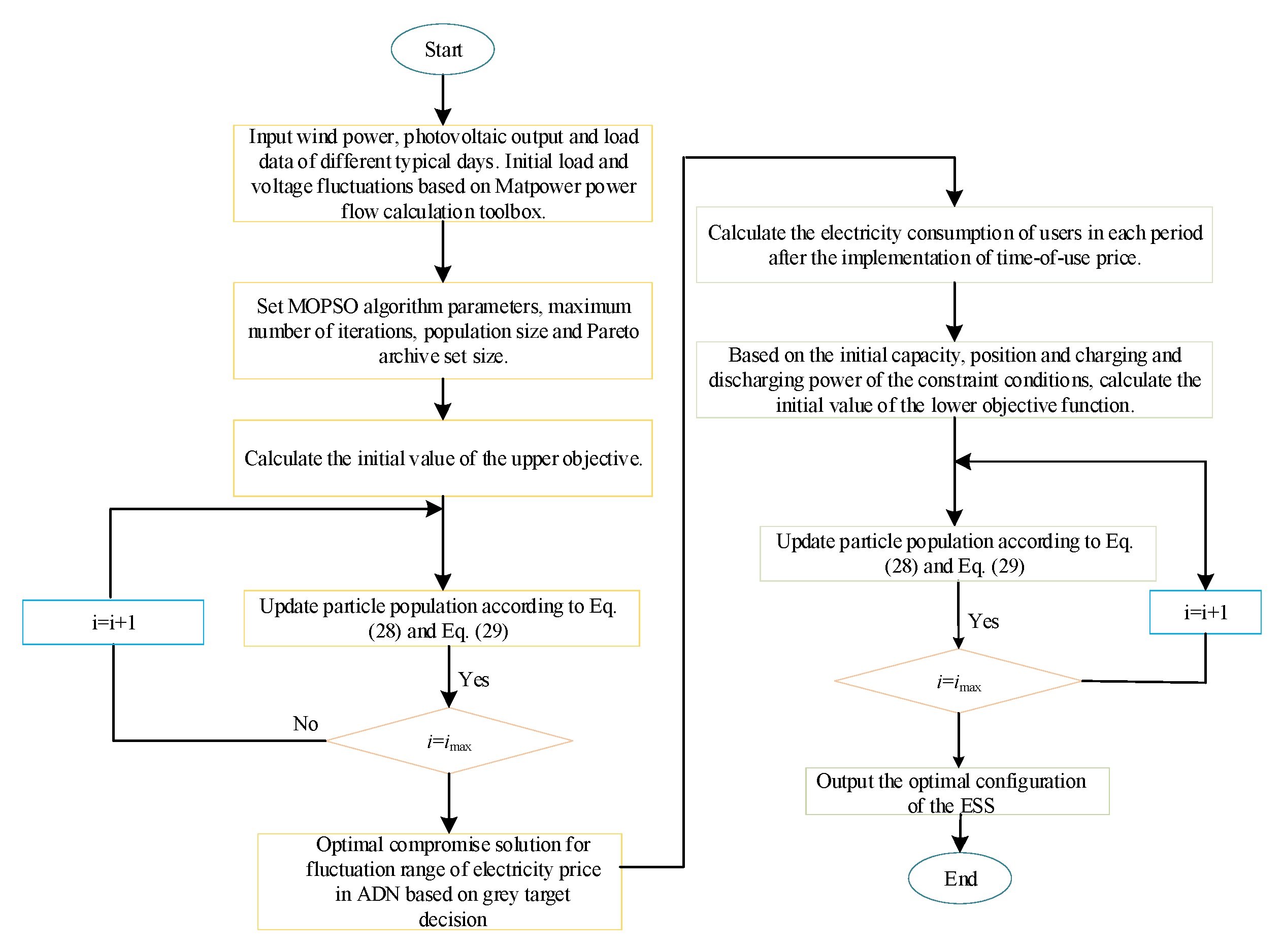
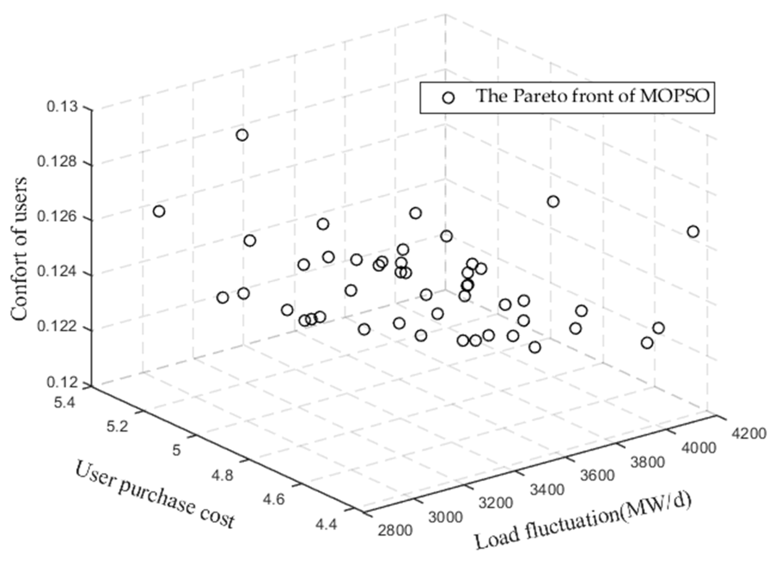
6.1. Model Solving Method Based on MOPSO

The location and capacity of the electricity–hydrogen hybrid system considering DR is a complex multi-objective model, which needs to optimize the electricity price fluctuation, ESS charging and discharging power, capacity, and location during each period. Therefore, this work uses MOPSO to solve the model [28,29]. The bi-layer model solving the process of the MOPSO algorithm is shown in Figure 1. Equations (29) and (30) represent MOPSO’s optimization mechanism.

$$v_i\left(t+1\right)=w{v}_i\left(t\right)+r_1{c}_1\left(\mathrm{P}bes{t}_i\left(t\right)-x_i\left(t\right)\right)+r_2{c}_2\left(\mathrm{G}bes{t}_i\left(t\right)-x_i\left(t\right)\right)$$

(29)

$$x_i\left(t+1\right)=x_i\left(t\right)+v_i\left(t+1\right)$$

(30)

where $\mathrm{P}bes{t}_i\left(t\right)$ represents the historical optimal position of the $i\left(i=1,2,3,\dots ,N\right)$ particles in the search process, which is the local optimal solution; $\mathrm{G}bes{t}_i\left(t\right)$ represents the optimal position of all particles in the current search results, which is the global optimal solution; $r_1$ and $r_2$ represent random values in [0,1]; $c_1$ and $c_2$ represent the particle self and group learning factors, usually between 0 and 2; $w$ represents the value of the inertia weight that controls the particles in the population to search in the solution space. The bi-level model solution flow based on the MOPSO algorithm is shown in Figure 2

6.2. A Compromise Solution Selection Method Based on Improved Grey Target Decision

In order to avoid the influence of subjective factors on the results, this work uses the improved grey target decision making (IGTDM) based on the entropy weight method (EWM) to obtain the optimal compromise solution. The detailed steps can be found in [30,31].

7. Case Studies

7.1. Simulation Experiment Model

This work designs a simulation experiment based on the extended IEEE-33 node test system [32]. The system topology is shown in Figure 3. Meanwhile, this work accesses two wind DGs with an installed capacity of 1 MW as well as two photovoltaic DGs with an installed capacity of 0.9 MW at nodes 15 and 32 as well as 23 and 20, respectively. In addition, the main parameters of ADN are shown in

Table 1. Parameters of ADN.

The Parameter of ADN	Value
System reference capacity	10 MVA
Load power	(3715 + j2300) kVA
Voltage reference value	12.66 kV

, whilst the main parameters of the different algorithms are shown in

Table 2. Main parameters of different algorithms.

Algorithm	Main Parameters	Value
MOPSO	Self-learning factor	1.4962
	Group learning factor	1.4962
	Maximum inertia factor	0.9
	Minimum inertia factor	0.4
MODE	Scaling factor	0.9
	Cross factor	0.4
	Generation boundary	10,000
MOABC	Food source improvement factor	5

. The main parameters of the algorithms can be deduced from a uniform design, as determined in [33,34,35].

Table 3. Main cost of ESS.

ESS Type	Parameters	Value
BESS	The cost of battery	1000 (USD/kW h)
	The cost of converter	700 (USD/kW)
	Charge efficiency	96%
	Discharge efficiency	96%
HESS	The cost of EC	900 (USD/kW)
	The cost of FC	430(USD/kW)
	The cost of HT	10 (USD/kg)
	EC efficiency	68%
	FC efficiency	65%

shows the main cost of ESS [36,37,38,39]. It should be noted that the installation node position of DG in this paper was completed before configuring ESS by referring to the previous work [40] and the method in the literature [41].

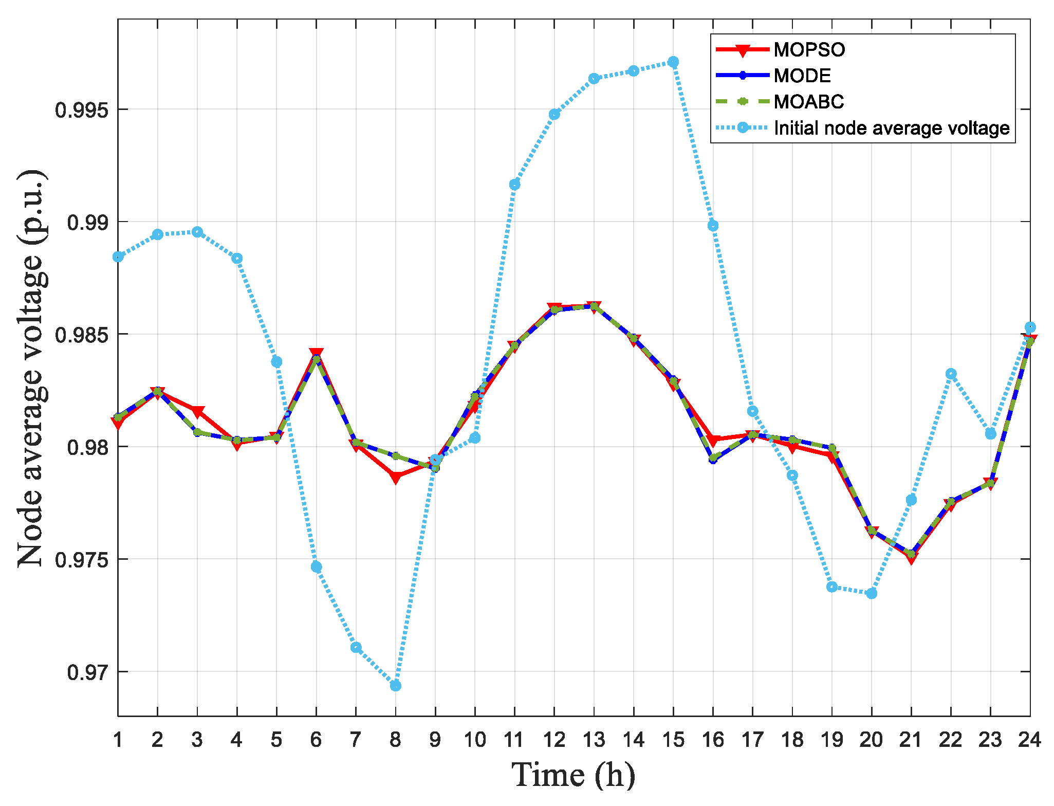
7.2. Analysis of Simulation Experiment Results

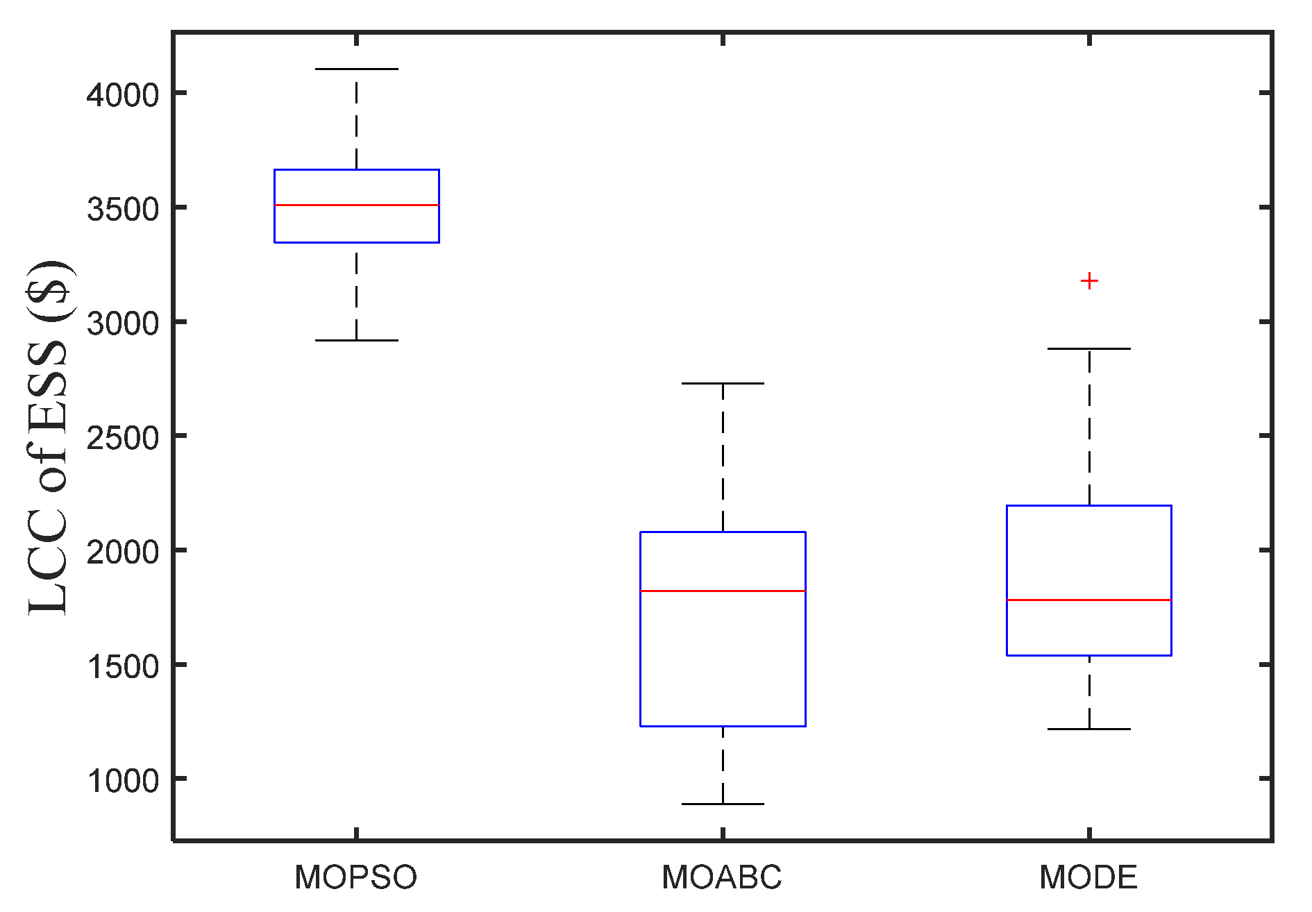
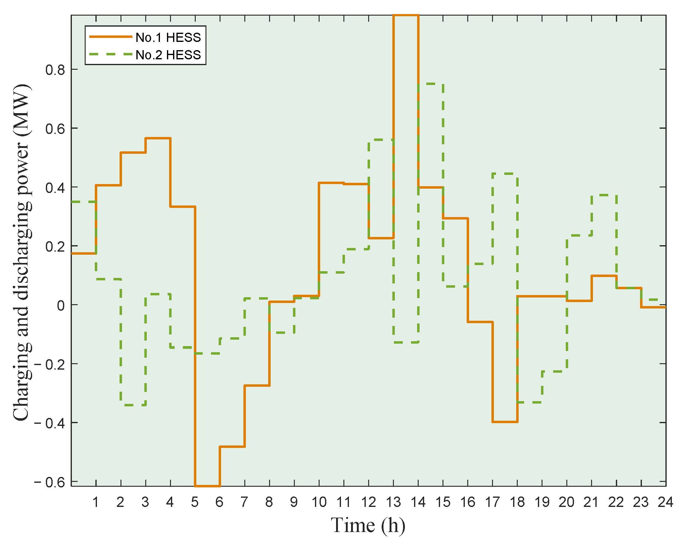
7.2.1. ESS Configuration Scheme

The optimization results of the upper-level model are shown in

Table 4. Optimization results of the upper model.

	Load Fluctuation (MW/Day)	User Purchase Cost Satisfaction Index	Comfort of User
Ordinary electricity price	7.7528	1.0	0
Time-of-use electricity price formulated by MOPSO	7.0885	0.8666	0.0057
Time-of-use electricity price formulated by MODE	7.0758	0.8677	0.0053
Time-of-use electricity price formulated by MOABC	7.0526	0.8762	0.0050

. Residents can achieve the maximum improvement in load fluctuation within a reasonable range of electricity comfort through the lower purchase cost than without considering the time of use electricity price based on the new price scheme formulated by MOPSO, MOABC, and MODE, respectively. In addition, the optimal configuration scheme formulated by different algorithms of ESS based on IGTDM is shown in

Table 5. Optimization results of the lower model of the MOPSO.

Configuration Scheme of ESS						Objective Function of Lower Model
BESS	ESS serial number	Nodes	Rated power (MW)	Capacity (MWh)	/	LCC (USD/day)	Load fluctuation (MW/day)	Voltage fluctuation (p.u./day)
	No.1 BESS	25	0.4972	1.4421	/	3.2855 × 103	4.8795	0.1246
	No.2 BESS	28	0.4869	1.4901	/
HESS	ESS serial number	Nodes	Rated power of FC (MW)	Rated power of EC (MW)	Capacity of HT (kg)
	No.1 HESS	12	0.6164	0.9830	108.15
	No.1 HESS	10	0.3410	0.7506	146.16

,

Table 6. Optimization results of the lower model of the MODE.

Configuration Scheme of ESS						Objective Function of Lower Model
BESS	ESS serial number	Nodes	Rated power (MW)	Capacity (MWh)	/	LCC (USD/day)	Load fluctuation (MW/day)	Voltage fluctuation (p.u./day)
	No.1 BESS	2	0.3307	0.7217	/	1.9522 × 103	6.3137	0.2126
	No.2 BESS	6	0.2336	0.5000	/
HESS	ESS serial number	Nodes	Rated power of FC (MW)	Rated power of EC (MW)	Capacity of HT (kg)
	No.1 HESS	7	0.2446	0.6250	28
	No.1 HESS	10	0.2474	0.8204	44.49

and

Table 7. Optimization results of the lower model of the MOABC.

Configuration Scheme of ESS						Objective Function of Lower Model
BESS	ESS serial number	Nodes	Rated power (MW)	Capacity (MWh)	/	LCC (USD/day)	Load fluctuation (MW/day)	Voltage fluctuation (p.u./day)
	No.1 BESS	2	0.1639	0.5000	/	1.3675 × 103	6.8495	0.2292
	No.2 BESS	8	0.2083	0.5000	/
HESS	ESS serial number	Nodes	Rated power of FC (MW)	Rated power of EC (MW)	Capacity of HT (kg)
	No.1 HESS	2	0.0581	0.3000	31.43
	No.1 HESS	31	0.4458	0.5883	28

. From Table 5, Table 6 and Table 7, it can be concluded that ESS based on the MOPSO configuration can most significantly reduce the load fluctuation and voltage fluctuation of ADN. Compared with MODE and MOABC, the net load fluctuation of ESS based on MOPSO is reduced by 22.93% and 28.76%, respectively. Meanwhile, the voltage fluctuation is reduced by 41.39% and 45.64%, respectively. In summary, although the LCC optimized by MOPSO is slightly higher than the other two algorithms, the stability of ADN can be most significantly improved by ESS based on MOPSO configuration. Therefore, according to the above configuration scheme, four ESSs are configured near the distributed power supply, which cannot quickly suppress the influence of the unstable output of DG on the stability of ADN. Figure 4 and Figure 5 are the load and voltage fluctuation curves of ADN after ESS access under the condition of considering DR. It should be noted that the average node voltage in Figure 5 is averaged by the node voltage values of all nodes. Based on the above, it can be concluded that the reasonable configuration of the ESS can stabilize the load and improve the stability of ADN.

Furthermore, in order to verify its superiority, MOPSO was analyzed from two aspects, namely computational stability and operation time. The computational stability of the three algorithms was shown by the boxplot in Figure 6, Figure 7 and Figure 8. It can be seen that the distribution of three objective functions optimized by MOPSO is more concentrated, indicating that the MOPSO algorithm is more stable and accurate in the ESS location, capacity, and power optimization.

Table 8. Comparison of the calculation times of the three algorithms.

Algorithm	Operation Time
MOPSO	86 min and 8 s
MODE	100 min and 21 s
MOABC	83 min and 1 s

shows the operation time of the three algorithms under the same population size (50) and iteration number (200). It can be concluded from the table that the operation time of MOABC and MOPSO is much lower than that of MODE. Figure 9 and Figure 10 are the operation curves of ESS. In this work, the ESS daily initial charge and discharge power is positive for ESS charging or for discharging. In addition, Figure 9 and Figure 10 show the charge–discharge power curve of both HESS and BESS in one day, respectively. These ESSs operate independently, so they can be charged and discharged simultaneously. It can be seen from the diagram that, compared with BESS, HESS does not have the ability of BESS to quickly swallow discharge because of its low conversion efficiency. However, due to its advantages of a long storage time and long running life, it can fully make up for the shortcomings of the short life of BESS.

Figure 11 and Figure 12 represent the Pareto front obtained by MOPSO. The distribution of the Pareto front reflects the distribution of solutions. In addition, by observing the Pareto front distribution of the upper-level objective function, it can be seen that user comfort is negatively correlated with the user purchase cost and load fluctuation, respectively. From the lower-level Pareto front distribution, it can be seen that LCC is also negatively correlated with voltage fluctuation and load fluctuation, which shows that the LCC of the hybrid ESS is often optimized at the expense of ADN stability. In summary, MOPSO can obtain a wide range of non-dominated solutions, which shows that MOPSO does not easily fall into a local optimum and has a superior optimization ability when solving ESS planning problems [42].

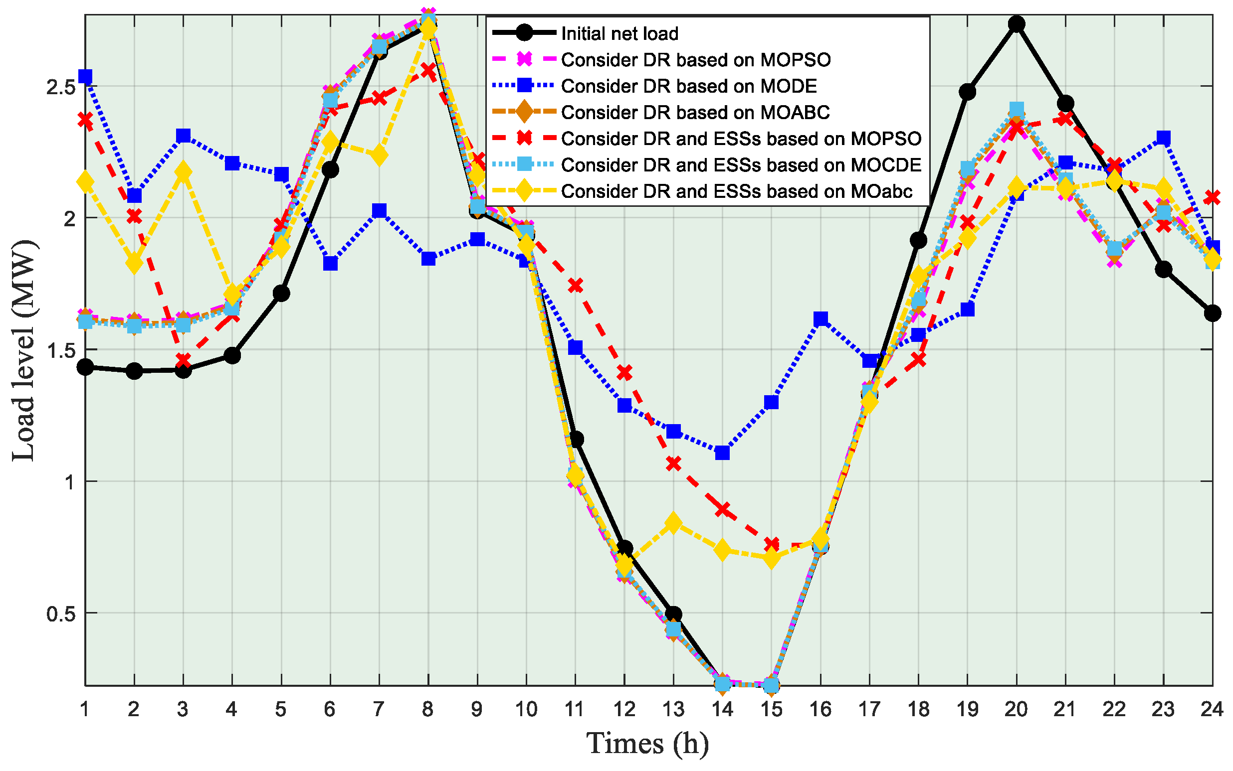
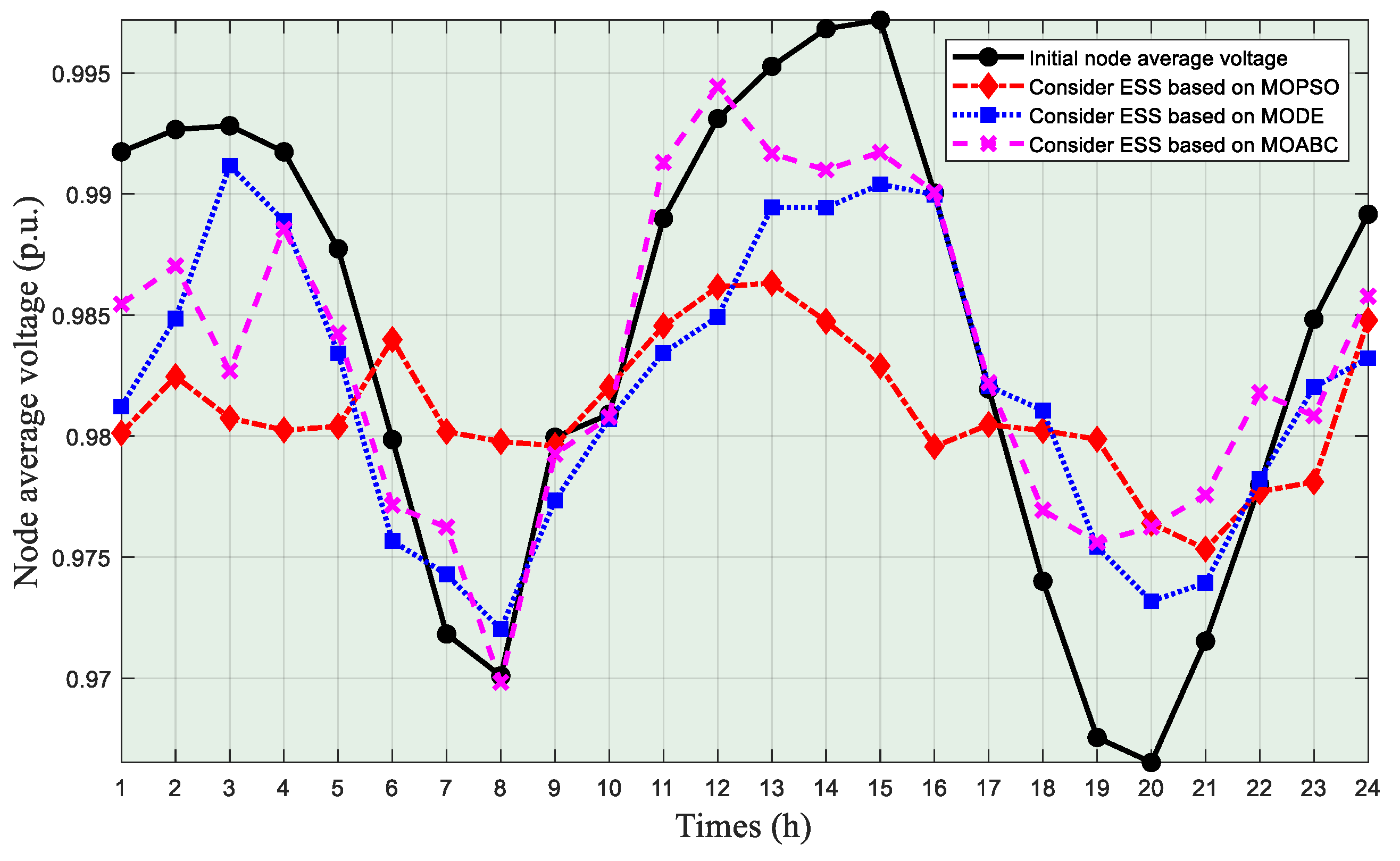
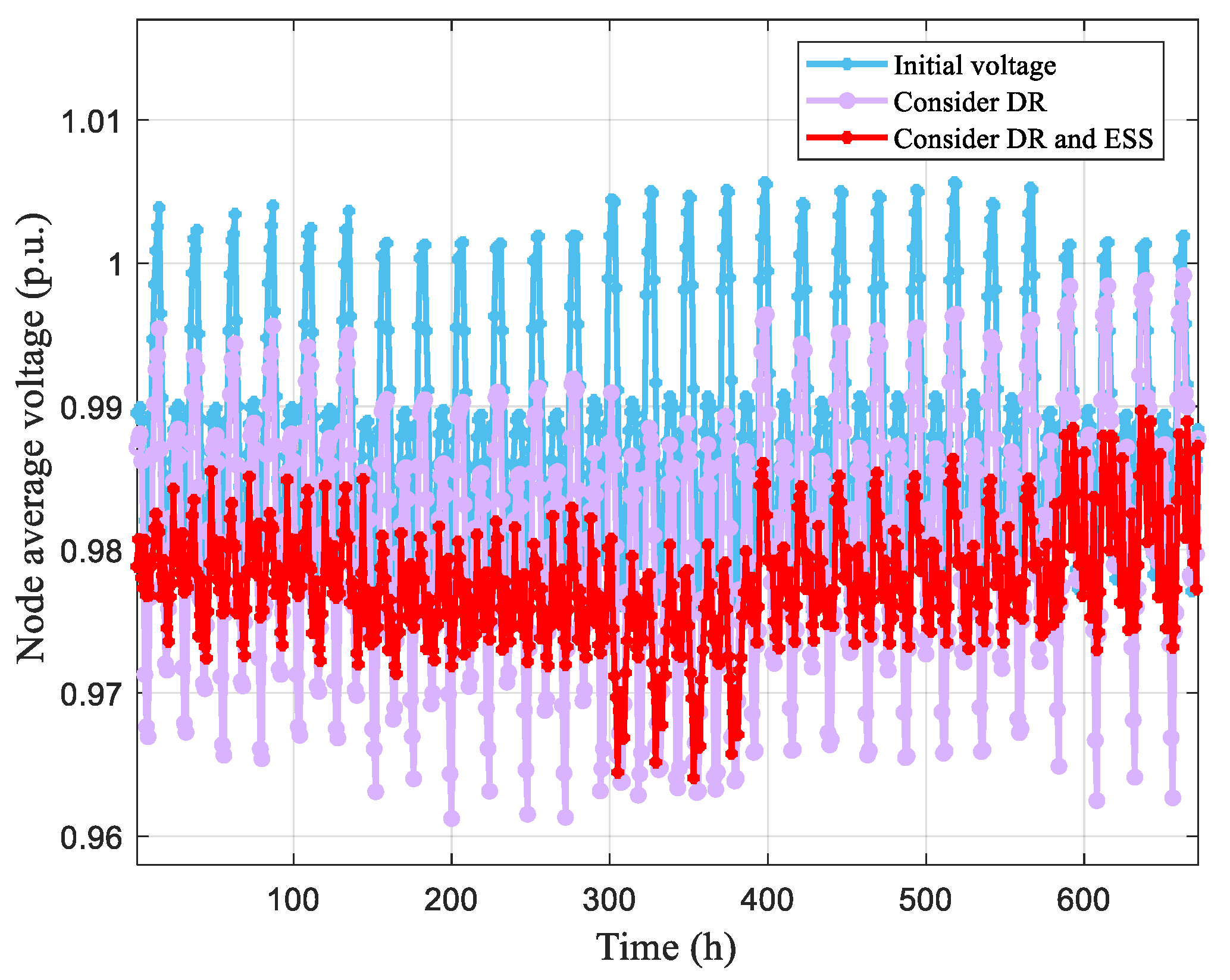
7.2.2. Analysis of the Stability of ADN throughout Four Weeks

To verify the feasibility of the system, the obtained results (the locations, capacities, and charging/discharging power of BESS and HESS in 24 h) by MOPSO-IGTDM were applied to analyze the stability of ADN. The curves of the load and voltage over the course of four weeks are shown in Figure 13 and Figure 14, respectively. Meanwhile, Table 5 gives the values of the load and voltage fluctuation. It can be concluded from

Table 9. Value of load and voltage fluctuation through four weeks.

	Net Load Fluctuation/(MW)	Voltage Fluctuation/(p.u.)
Initial	206.51	0.2663
Consider DR	190.47	0.2969
After ESS access	153.05	0.1470

that the net load fluctuation and voltage fluctuation decreased by 25.89% and 44.80% after accessing ESS compared with the initial condition, respectively. On the whole, the stability of ADN can be greatly enhanced by taking the DR and ESS into account at the same time.

7.2.3. Influence of Different Operation Modes on Stability of ADN

Based on the time-of-use price strategy and ESS configuration, this section divides the ADN operation into four scenarios to compare the stability of ADN in different scenarios. Scenario 1: DR is not considered and ESS is not configured; Scenario 2: Consider DR only; Scenario 3: Configure ESS only; Scenario 4: Consider DR and configure ESS.

Table 10. Configuration of ADN stability and ESS under different scenarios.

Operation Scenarios	Configuration Scheme of BESS			Configuration Scheme of HESS				Objective Function of Lower Model
	Nodes	Rated Power (MW)	Capacity (MWh)	Nodes	Rated Power of FC (MW)	Rated Power of EC (MW)	Capacity of HT (kg)	LCC (USD/Day)	Load Fluctuation (MW/Day)	Voltage Fluctuation (p.u./Day)
Scenario 1	/								7.7258	0.3318
Scenario 2	/								7.0885	0.2843
Scenario 3	[7 19]	[0.9718 0.2773]	[4.000 0.8656]	[28 11]	[0.3818 0.2796]	[1.000 0.9908]	[102.19 59.55]	3.4581 × 103	6.5552	0.1745
Scenario 4	[25 28]	[0.4972 0.4869]	[1.4421 1.4901]	[12 10]	[0.6164 0.3410]	[0.9830 0.7506]	[108.15 146.16]	3.2855 × 103	4.8795	0.1246

shows the ADN stability and ESS configuration under different operating scenarios. In addition, it can be seen from Table 5 that the LCC of ESS is unaffected by DR. In addition, comparing Scenario 1 and Scenario 2 in Table 10, it can be seen that considering DR without ESS, the ADN load fluctuation is reduced by 0.6373 (MW/day) and the voltage fluctuation is reduced by 0.0475 (p.u./day). Comparing the LCC values of Scenario 3 and Scenario 4, it can be seen that configuring ESS after considering DR can reduce the LCC of the configured ESS by 172.6 (USD/day), and the load fluctuation and voltage fluctuation are reduced by 1.6757 (MW/day) and 0.0499 (p.u./day), respectively. Moreover, comparing scenario 2 and scenario 4, configuring ESS while considering DR can further reduce the ADN, 13.44% load fluctuation and 0.72% voltage fluctuation. This is because the application of the time-of-use electricity price changes the user’s electricity consumption behavior and improves the stability of ADN operation. On this basis, the further configuration of ESS can give full play to the role of ESS and greatly reduce the load fluctuation and voltage fluctuation of ADN. Therefore, configuring ESS while considering DR can maximize the operational stability of ADN.

8. Discussion

8.1. Effect on Voltage Quality

The access to DG and BESS changes the power flow distribution of the ADN, which also has a certain impact on the voltage quality of the ADN. When DG and BESS are connected to ADN at the same time, and ADN loss is ignored and the node voltage can be calculated by the following equation (assuming that node No.1 is the power injection node of DG and BESS, and that node No.0 is the access node of the upper power grid):

$$\{\begin{array}{c}{U}_{\mathrm{node}}^{’}=U_0-\Delta U_{\mathrm{node}}^{’}\\ \Delta U_{\mathrm{node}}^{’}=\frac{\left(P_{\mathrm{load}}-P_{\mathrm{DG}}+P_{\mathrm{BESS}}\right)·R_{\mathrm{node}}+\left(Q_{\mathrm{load}}-Q_{\mathrm{DG}}+Q_{\mathrm{BESS}}\right)·X_{\mathrm{node}}}{U_0}\end{array}$$

(31)

where $P_{\mathrm{load}}$ and $Q_{\mathrm{load}}$ represent the active power and reactive power of the load, respectively. $U_{\mathrm{N}}$ represents the phase voltage of the ADN. $P_{\mathrm{DG}}$ and $Q_{\mathrm{DG}}$ represent the active power and reactive power transferred to the ADN by DG. $P_{\mathrm{BESS}}$ and $Q_{\mathrm{BESS}}$ represent the active and reactive power absorbed or emitted by BESS to the ADN, which is positive when BESS is charging and negative when it is discharging. $U_{\mathrm{node}}^{’}$ and $\Delta U_{\mathrm{node}}^{’}$ are the voltage at node 1 and the voltage drop of 0–1 branch after accessing DG and BESS, respectively.

After the BESS ‘s appropriate capacity is connected, it absorbs power from the ADN as a load in the charging state to avoid overvoltage in node 1. Therefore, BESS can reduce the voltage surge caused by the access of large-capacity DG through reasonable charging and discharging. Similarly, if the ADN is at peak load and the DG output is insufficient, BESS can act as the power supply to send power to the ADN and increase the node voltage. Therefore, for the ADN with a high proportion of DG access, the access of BESS can effectively guarantee the voltage level of the ADN and improve the quality of the power supply. The rational allocation of BESS capacity is the key to exerting the pressure regulation capability of BESS.

The influence of different access location conditions on voltage fluctuation is verified by only changing the location of BESS when the capacity did not change.

Table 11. Voltage fluctuation at different access locations of BESS.

Algorithm	Nodes of BESS	Voltage Fluctuation/(p.u.)
MOPSO	[2 6]	0.1246
MODE	[2 8]	0.1255
MOABC	[2 31]	0.1254

shows the values of voltage fluctuation when BESS is connected to the optimal location obtained by MODE and MOABC under the condition of constant capacity and charge–discharge power, respectively. When node 2 and node 6 are connected to BESS, the voltage fluctuation decreases by 0.72% and 0.64% compared with the two other conditions, respectively. Figure 15 is the curve of voltage fluctuation at different access locations of BESS. On the whole, it can be seen that the proposed model is feasible and the algorithm is superior.

8.2. Effect on the Load Level

$$P_{\mathrm{L}}\left(t\right)=P_{\mathrm{load}}\left(t\right)-P_{\mathrm{DG}}\left(t\right)+P_{\mathrm{dis}/\mathrm{chaD},\mathrm{BESS}}\left(t\right)$$

(32)

where $P_{\mathrm{L}}\left(t\right)$ represents the equivalent load power of ADN at time $t$ when DG and BESS are connected simultaneously. $P_{\mathrm{load}}\left(t\right)$ represents the load demand of ADN at time $t$.

It can be seen that BESS can effectively balance the power supply and demand and reduce the peak–valley load difference. However, the peak cutting and valley filling effects of BESS largely depend on the configured capacity and its charging and discharging strategy.

9. Conclusions

In this work, the DR model is established based on the time-of-use electricity price strategy, and a bi-layer model for configuring the electricity–hydrogen hybrid ESS is established based on the DR model. The conclusion is as follows:

(1) The time-of-use price strategy can achieve a balance between the stability of the ADN and the comfort of the user side through the load transfer of the ADN, and the load transfer operation will not change the total power consumption throughout the day.

(2) The bi-layer ESS location and capacity model proposed in this work not only considers the profits of all parties but also improves the stability of ADN by scientifically and reasonably planning the capacity and access location of ESS.

(3) A simulation experiment based on the IEEE-33 node test system is designed. In the simulation experiment result, the stability of ADN can be greatly enhanced by the configuration scheme based on MOPSO. Compared with MODE and MOABC, the net load fluctuation of ESS based on MOPSO is reduced by 22.93% and 28.76%, respectively. Meanwhile, the voltage fluctuation is reduced by 41.39% and 45.64%, respectively. The comparison of ADN operation indexes in four different scenarios is given. The experimental results show that the electricity–hydrogen hybrid energy storage system can effectively reduce the ADN load fluctuation and voltage fluctuation. Considering DR while configuring ESS, the load fluctuation and voltage fluctuation of ADN can be further reduced.

In future research, it is not only necessary to consider how ESS can be more correctly connected to ADN, but also whether the multi-type ESS comprehensive configuration can further reduce the configuration cost and improve the stability of ADN operation.

References

1. Yang, B.; Li, J.; Shu, H.; Cai, Z.; Tang, B.; Huang, X.; Zhu, M. Recent advances of optimal sizing and location of charging stations: A critical overview. Int. J. Energy Res. 2022, 43, 17899–17925. [Google Scholar] [CrossRef]
2. Yang, B.; Wang, J.; Cao, P.; Zhu, T.; Shu, H.; Chen, J.; Zhang, J.; Zhu, J. Classification, summarization and perspectives on state-of-charge estimation of lithium-ion batteries used in electric vehicles: A critical comprehensive survey. J. Energy Storage 2021, 32, 102572. [Google Scholar] [CrossRef]
3. Yang, B.; Wang, J.; Chen, Y.; Li, D.; Zeng, C.; Chen, Y.; Guo, Z.; Shu, H.; Zhang, X.; Yu, T.; et al. Optimal sizing and placement of energy storage system in power grids: A state-of-the-art one-stop handbook. J. Energy Storage 2020, 32, 101814. [Google Scholar] [CrossRef]
4. Yang, B.; Liu, B.; Zhou, H.; Wang, J.; Yao, W.; Wu, S.; Shu, H.; Ren, Y. A critical survey of technologies of large offshore wind farm integration: Summarization, advances, and perspectives. Prot. Control Mod. Power Syst. 2022, 7, 17. [Google Scholar] [CrossRef]
5. Xu, B.; Zhang, G.; Li, K.; Li, B.; Chi, H.; Yao, Y.; Fan, Z. Reactive power optimization of a distribution network with high-penetration of wind and solar renewable energy and electric vehicles. Prot. Control Mod. Power Syst. 2022, 7, 51. [Google Scholar] [CrossRef]
6. Fu, X.; Wu, X.; Zhang, C.; Fan, S.; Liu, N. Planning of distributed renewable energy systems under uncertainty based on statistical machine learning. Prot. Control Mod. Power Syst. 2022, 7, 41. [Google Scholar] [CrossRef]
7. Murty, V.V.S.N.; Kumar, A. Retraction Note: Multi-objective energy management in microgrids with hybrid energy sources and battery energy storage systems. Prot. Control Mod. Power Syst. 2022, 7, 11. [Google Scholar] [CrossRef]
8. Yang, J.J.; Cheng, R.F.; Xu, L.B. Multi-objective optimization simulation of active distribution network considering new energy access. Comput. Simul. 2022, 39, 108–113. [Google Scholar]
9. Zhu, P.X.; Guo, Q.; Li, L.Z.; Zheng, D.; Cai, H. Distributed energy storage configuration considering the vulnerability of active distribution network. Electr. Meas. Instrum. 2023, 1–8. Available online: http://kns.cnki.net/kcms/detail/23.1202.TH.20221019.1512.014.html (accessed on 20 October 2022).
10. Yue, Y.Y.; Wang, Z.D.; Wang, H.; Luo, X.; Su, Z.; Hui, Z.J. Day-Ahead Optimal Dispatch for Active Distribution Network Considering the Action Cost of Devices. Electr. Power 2023, 1–12. Available online: http://kns.cnki.net/kcms/detail/11.3265.tm.20221221.0945.002.html (accessed on 23 December 2022).
11. Yang, P.; Yu, D.; Guo, Y.H.; Zhang, S.C. Optimization model of new energy accommodation considering demand response. Distrib. Util. 2022, 39, 79–86. [Google Scholar] [CrossRef]
12. Ding, W.; Yuan, J.H.; Hu, Z.G. Time-of-use price decision model considering users reaction and satisfaction index. Power Syst. Autom. 2005, 29, 10–14. [Google Scholar]
13. Yang, H.Z.; Li, M.L.; Jiang, Z.Y. Optimal operation of regional integrated energy system considering demand side electricity heat and natural-gas loads response. Power Syst. Prot. Control 2020, 48, 30–37. [Google Scholar] [CrossRef]
14. Li, Z.L.; Liu, R.H. Operation optimization of regional integrated energy system with energy storage considering demand response. Mod. Electr. Power 2019, 36, 61–67. [Google Scholar] [CrossRef]
15. Zhang, C.; Zuo, G.; Teng, Z.S. Optimal dispatch of distribution network considering demand response. Intell. Sched. 2020, 48, 53–58. [Google Scholar]
16. Zhao, F.; Xue, L.J.; Zhu, J.L. An energy storage capacity allocation method for power system based on improved particle swarm optimization. Zhejiang Electr. Power 2022, 41, 17–22. [Google Scholar] [CrossRef]
17. An, D.; Yang, D.Y.; Wu, W.L.; Cai, W.; Li, H.; Yang, B.; Han, Y. Optimal location and sizing of battery energy storage systems in a distribution network based on a modified multi-objective mayfly algorithm. Power Syst. Prot. Control 2022, 50, 1–39. [Google Scholar] [CrossRef]
18. Ding, Q.; Zeng, P.L.; Sun, Y.K. A planning method for the placement and sizing of distributed energy storage system considering the uncertainty of renewable energy sources. Energy Storage Sci. Technol. 2020, 9, 162–169. [Google Scholar] [CrossRef]
19. Xu, C.B.; Liu, J.G. Hydrogen energy storage in China’s new-type power system: Application value, challenges, and prospects. Strateg. Study CAE 2022, 24, 89–99. [Google Scholar] [CrossRef]
20. Qiu, B.; Mu, H.B.; Wang, K.; Zhang, Z.C.; Yang, Z. Optimal dispatching of hydrogen coupling IES considering mixed transmission of hydrogen and natural gas. Proc. CSU-EPSA 2022, 34, 51–59. [Google Scholar] [CrossRef]
21. Zhou, Z.L. Energy efficiency analysis of hydrogen storage coupled gas-steam combined cycle. Acta Energ. Sol. Sin. 2021, 42, 39–45. [Google Scholar] [CrossRef]
22. Wang, Y.; Zhang, Y.; Xue, L.; Liu, C.; Song, F.; Sun, Y.; Che, B. Research on planning optimization of integrated energy system based on the differential features of hybrid energy storage system. J. Energy Storage 2022, 55, 105368. [Google Scholar] [CrossRef]
23. Chen, Y.; Shi, Y.F.; Zhong, H.M.; Wang, X.; Lei, X.; Yin, H.; Liu, X. Configuration method for hydrogen-electricity hybrid energy storage system in transmission grid with high proportion of PV and wind power connection. Electr. Power Constr. 2022, 43, 85–98. [Google Scholar] [CrossRef]
24. Chen, C.; Hu, B.; Xie, K.; Wan, L.; Xiang, B. A peak-valley TOU price model considering power system reliability and power purchase risk. Power Grid Technol. 2014, 38, 2141–2148. [Google Scholar] [CrossRef]
25. Guizhou Provincial Development and Reform Commission. Notice of Provincial Development and Reform Commission on Matters Related to the Trial of Peak and Valley TOU Electricity Price [EB/OL]. (31 August 2021). Available online: http://fgw.guizhou.gov.cn/zwgk/gzhgfxwjsjk/gfxwjsjk/202110/t20211019_70938120.html (accessed on 9 November 2022).
26. Harvey, H.L.D. Clarifications of and improvements to the equations used to calculate the levelized cost of electricity (LCOE), and comments on the weighted average cost of capital (WACC). Energy 2020, 207, 118340. [Google Scholar] [CrossRef]
27. Xue, J.H.; Ye, J.L.; Tao, Q.; Wang, D.; Sang, B.; Yang, B. Economic feasibility of user-side battery energy storage based on whole-life-cycle cost model. Power Grid Technol. 2016, 40, 2471–2476. [Google Scholar] [CrossRef]
28. Feng, L.; Kong, Q.Y.; Guo, L. An algorithm for Short-term Electrical Load Forecasting Based on Multi-objective Particle Swarm Optimization. Power Syst. Technol. 2006, S2, 265–268. [Google Scholar] [CrossRef]
29. Huang, S.; Wang, Y.; Ji, Z.C. Dynamic multiple-fuels economic environmental dispatch using multi-objective particle swarm optimization. Control Decis. 2018, 33, 1255–1263. [Google Scholar] [CrossRef]
30. Zhuo, Y.; Yang, Z.; Cai, W.; Zhou, B. Multi-objective optimal configuration of electricity-hydrogen hybrid energy storage system in zero-carbon park. Electr. Power Constr. 2022, 43, 1–12. [Google Scholar] [CrossRef]
31. Yang, H.H.; Wang, J.; Tai, N.; Ding, Y. Robust optimization of distributed generation in a microgrid based on grey target decision-making and multi-objective cuckoo search algorithm. Power Syst. Prot. Control 2019, 47, 20–27. [Google Scholar] [CrossRef]
32. Yang, B.; Yu, L.; Chen, Y.; Ye, H.; Shao, R.; Shu, H.; Sun, L. Modelling, applications, and evaluations of optimal sizing and placement of distributed generations: A critical state-of-the-art survey. Int. J. Energy Res. 2020, 45, 3615–3642. [Google Scholar] [CrossRef]
33. Lu, L.M.; Chu, G.W.; Zhang, T.; Yang, Z.C. Optimal configuration of energy storage in a microgrid based on improved multi-objective particle swarm optimization. Power Syst. Prot. Control 2020, 48, 116–124. [Google Scholar]
34. Akbari, R.; Hedayatzadeh, R.; Ziarati, K.; Hassanizadeh, B. A multi-objective artificial bee colony algorithm. Swarm Evol. Comput. 2012, 2, 39–52. [Google Scholar] [CrossRef]
35. Reynoso-Meza, G. Multi-objective Differential Evolution Algorithm with Spherical Pruning with-MATLAB Central File Exchange. Available online: https://ww2.mathworks.cn/matlabcentral/fileexchange/39215-multi-objective-differential-evolution-algorithm-with-spherical-pruning?s_tid=ta_fx_results (accessed on 27 November 2012).
36. Yan, Y.; Zhang, C.H.; Li, K.; Wang, Z. An integrated design for hybrid combined cooling, heating and power system with compressed air energy storage. Energy 2018, 210, 1151–1166. [Google Scholar] [CrossRef]
37. Liu, J.; Cao, S.; Chen, X.; Yang, H.; Peng, J. Energy planning of renewable applications in high-rise residential buildings integrating battery and hydrogen vehicle storage. Appl. Energy 2021, 281, 116038. [Google Scholar] [CrossRef]
38. David, B.; Paolo, M.; Domenico, F.; Kyrre, S. Massimo santarelli. life cycle environmental analysis of a hydrogen-based energy storage system for remote applications. Energy Rep. 2022, 8, 5080–5092. [Google Scholar] [CrossRef]
39. Si, Y.; Chen, L.; Chen, X.; Gao, M.; Ma, L.; Mei, S. Optimal capacity allocation of hydrogen energy storage in wind-hydrogen hybrid system based on distributionally robust. Power Autom. Equip. 2021, 41, 3–10. [Google Scholar] [CrossRef]
40. Yang, B.; Yu, L.; Wang, J.T.; Shu, H.; Cao, P.; Yu, T. Optimal sizing and placement of distributed generation using adaptive manta ray foraging optimization. J. Shanghai Jiaotong Univ. 2021, 55, 1673–1688. [Google Scholar] [CrossRef]
41. Ankit, U.; Saumendra, S. Optimal network reconfiguration and DG allocation using adaptive modified whale optimization algorithm considering probabilistic load flow. Electr. Power Syst. Res. 2021, 192, 106909. [Google Scholar] [CrossRef]
42. Zheng, C.L.; Wu, Y.J.; Chen, Y.Q.; Ye, J.W.; Zheng, T.; Wei, L.L.; Wu, S. Optimal Siting and Sizing of Energy Storage Based on Non-dominated Sorting of Improved Bat Algorithm. Distrib. Util. 2021, 38, 107–115. [Google Scholar] [CrossRef]
Figure 1. Active DR diagram.
Processes 11 00852 g001
Figure 2. The flowchart of the bi-level model based on MOPSO algorithm.
Processes 11 00852 g002
Figure 3. Topology of the extended IEEE-33 bus system.
Processes 11 00852 g003
Figure 4. Load curve connected to ESS considering DR.
Processes 11 00852 g004
Figure 5. Voltage curve connected to ESS considering DR.
Processes 11 00852 g005
Figure 6. Boxplot of LCC obtained by various algorithms.
Processes 11 00852 g006
Figure 7. Boxplot of net load fluctuation obtained by various algorithms.
Processes 11 00852 g007
Figure 8. Boxplot of voltage fluctuation obtained by various algorithms.
Processes 11 00852 g008
Figure 9. Charging and discharging power of HESS.
Processes 11 00852 g009
Figure 10. Charging and discharging power of BESS.
Processes 11 00852 g010
Figure 11. The Pareto front of the upper-level objective function.
Processes 11 00852 g011
Figure 12. The Pareto front of the lower-level objective function.
Processes 11 00852 g012
Figure 13. Load fluctuation throughout four weeks.
Processes 11 00852 g013
Figure 14. Voltage fluctuation throughout four weeks.
Processes 11 00852 g014
Figure 15. Voltage fluctuation at different access locations of BESS.
Processes 11 00852 g015